Cascaded Deep Monocular 3D Human Pose Estimation with Evolutionary Training Data
←
→
Page content transcription
If your browser does not render page correctly, please read the page content below
Cascaded Deep Monocular 3D Human Pose Estimation with Evolutionary
Training Data
Shichao Li1 , Lei Ke1 , Kevin Pratama1 , Yu-Wing Tai2 , Chi-Keung Tang1 , Kwang-Ting Cheng1
1
The Hong Kong University of Science and Technology, 2 Tencent
slicd@cse.ust.hk, timcheng@ust.hk
arXiv:2006.07778v3 [cs.CV] 9 Apr 2021
Abstract
End-to-end deep representation learning has achieved
remarkable accuracy for monocular 3D human pose esti-
mation, yet these models may fail for unseen poses with lim-
ited and fixed training data. This paper proposes a novel
data augmentation method that: (1) is scalable for syn-
Input Image
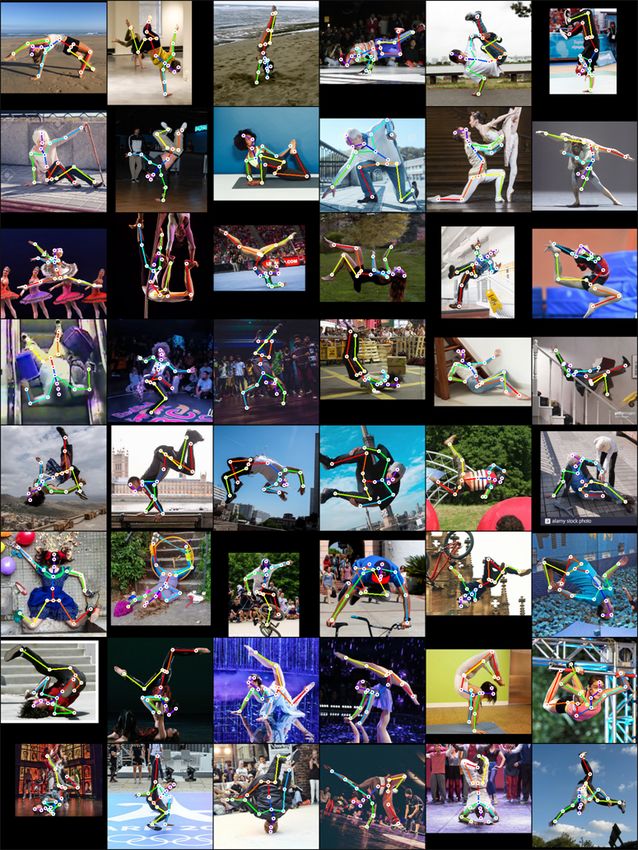
thesizing massive amount of training data (over 8 million Before Evolution (Ours)
valid 3D human poses with corresponding 2D projections)
for training 2D-to-3D networks, (2) can effectively reduce
dataset bias. Our method evolves a limited dataset to syn-
thesize unseen 3D human skeletons based on a hierarchi-
cal human representation and heuristics inspired by prior
knowledge. Extensive experiments show that our approach
not only achieves state-of-the-art accuracy on the largest
public benchmark, but also generalizes significantly better
to unseen and rare poses. Code, pre-trained models and Li et al. After Evolution (Ours)
tools are available at this HTTPS URL1 . Figure 1: Model trained on the evolved training data gener-
alizes better than [28] to unseen inputs.
1. Introduction
ronment and selected daily actions. Deep models can easily
Estimating 3D human pose from RGB images is crit-
exploit these bias but fail for unseen cases in unconstrained
ical for applications such as action recognition [36] and
environments. This fact has been validated by recent works
human-computer interaction, yet it is challenging due to
[74, 71, 28, 69] where cross-dataset inference demonstrated
lack of depth information and large variation in human
poor generalization of models trained with biased data.
poses, camera viewpoints and appearances. Since the
introduction of large-scale motion capture (MC) datasets To cope with the domain shift of appearance for 3D
[61, 22], learning-based methods and especially deep rep- pose estimation, recent state-of-the-art (SOTA) deep mod-
resentation learning have gained increasing momentum in els adopt the two-stage architecture [73, 14, 15]. The first
3D pose estimation. Thanks to their representation learn- stage locates 2D human key-points from appearance infor-
ing power, deep models have achieved unprecedented high mation, while the second stage lifts the 2D joints into 3D
accuracy [47, 44, 31, 37, 36, 65]. skeleton employing geometric information. Since 2D pose
annotations are easier to obtain, extra in-the-wild images
Despite their success, deep models are data-hungry and
can be used to train the first stage model, which effectively
vulnerable to the limitation of data collection. This prob-
reduces the bias towards indoor images during data collec-
lem is more severe for 3D pose estimation due to two fac-
tion. However, the second stage 2D-to-3D model can still be
tors. First, collecting accurate 3D pose annotation for RGB
negatively influenced by geometric data bias, yet not stud-
images is expensive and time-consuming. Second, the col-
ied before. We focus on this problem in this work and our
lected training data is usually biased towards indoor envi-
research questions are: are our 2D-to-3D deep networks in-
1 https://github.com/Nicholasli1995/EvoSkeleton fluenced by data bias? If yes, how can we improve network
1
generalization when the training data is limited in scale or        and employ two mainstream architectures: one-stage meth-
variation?                                                          ods [71, 74, 36, 47, 44, 31, 65, 18] and two-stage meth-
    To answer these questions, we propose to analyze the            ods [42, 37, 51, 73]. The former directly map pixel inten-
training data with a hierarchical human model and represent         sities to 3D poses, while the latter first extract intermediate
human posture as collection of local bone orientations. We          representation such as 2D key-points and then lift them to
then propose a novel dataset evolution framework to cope            3D poses.
with the limitation of training data. Without any extra an-             We adopt the discriminative approach and focus on the
notation, we define evolutionary operators such as crossover        2D-to-3D lifting network. Instead of using a fixed training
and mutation to discover novel valid 3D skeletons in tree-          dataset, we evolve the training data to improve the perfor-
structured data space guided by simple prior knowledge.             mance of the 2D-to-3D network.
These synthetic skeletons are projected to 2D and form 2D-          Weakly-supervised 3D human pose estimation. Super-
3D pairs to augment the data used for training 2D-to-3D             vised training of DNNs demands massive data while 3D
networks. With an augmented training dataset after evolu-           annotation is difficult. To address this problem, weakly-
tion, we propose a cascaded model achieving state-of-the-           supervised methods explore other potential supervision to
art accuracy under various evaluation settings. Finally, we         improve network performance when only few training data
release a new dataset for unconstrained human pose in-the-          is available [48, 53, 54, 25, 12, 70, 30]. Multi-view con-
wild. Our contributions are summarized as follows:                  sistency [48, 53, 54, 25, 12] is proposed and validated as
                                                                    useful supervisory signal when training data is scarce, yet a
  • To our best knowledge, we are the first to improve 2D-          minimum of two views are needed. In contrast, we focus on
    to-3D network training with synthetic paired supervi-           effective utilization of scarce training data by synthesizing
    sion.                                                           new data from existing ones and uses only single view.
  • We propose a novel data evolution strategy which can            Data augmentation for pose estimation. New images can
    augments an existing dataset by exploring 3D human              be synthesized to augment indoor training dataset [55, 68].
    pose space without intensive collection of extra data.          In [68] new images were rendered using MC data and hu-
    This approach is scalable to produce 2D-3D pairs in             man models. Domain adaption was performed in [11] dur-
    the order of 107 , leading to better model generalization       ing training with synthetic images. Adversarial rotation and
    of 2D-to-3D networks.                                           scaling were used in [50] to augment data for 2D pose es-
                                                                    timation. These works produce synthetic images while we
  • We present TAG-Net, a deep architecture consisting              focus on data augmentation for 2D-to-3D networks and pro-
    of an accurate 2D joint detector and a novel cascaded           duce synthetic 2D-3D pairs.
    2D-to-3D network. It out-performs previous monoc-               Pose estimation dataset. Most large-scale human pose es-
    ular models on the largest 3D human pose estimation             timation datasets [72, 32, 3] only provide 2D pose anno-
    benchmark in various aspects.                                   tations. Accurate 3D annotations [22, 61] require MC de-
                                                                    vices and these datasets are biased due to the limitation of
  • We release a new labeled dataset for unconstrained hu-
                                                                    data collection process. Deep models are prone to overfit
    man pose estimation in-the-wild.
                                                                    to these biased dataset [66, 67, 29], failing to generalize in
   Fig. 1 shows a 2D-to-3D network trained on our aug-              unseen situations. Our method can synthesize for free with-
mented dataset can handle rare poses while others such              out human annotation large amount of valid 3D poses with
as [28] may fail.                                                   larger coverage in human pose space.

2. Related Works                                                    3. Dataset Evolution
Monocular 3D human pose estimation. Single-image                        From a given input image xi containing one human sub-
3D pose estimation methods are conventionally categorized           ject, we aim to infer the 3D human pose p̂i given the im-
into generative methods and discriminative methods. Gen-            age observation φ(xi ). To encode geometric information as
erative methods fit parametrized models to image obser-             other 2D-to-3D approaches [37, 73, 28], we represent φ(x)
vations for 3D pose estimation. These approaches rep-               as the 2D coordinates of k human key-points (xi , yi )ki=1 on
resent humans by PCA models [2, 75], graphical mod-                 the image plane. As a discriminative approach, we seek
els [8, 5] or deformable meshes [4, 34, 7, 45, 26]. The             a regression function F parametrized by Θ that outputs
fitting process amounts to non-linear optimization, which           3D pose as p̂i = F(φ(xi ), Θ). This regression func-
requires good initialization and refines the solution iter-         tion is implemented as a DNN. Conventionally this DNN
atively. Discriminative methods [57, 1, 6] directly learn           is trained on a dataset collected by MC devices [61, 22].
a mapping from image observations to 3D poses. Re-                  This dataset consists of paired images and 3D pose ground
cent deep neural networks (DNNs) fall into this category            truths {(xi , pi )}N
                                                                                       i=1 and the DNN can be trained by gradi-

                                                                2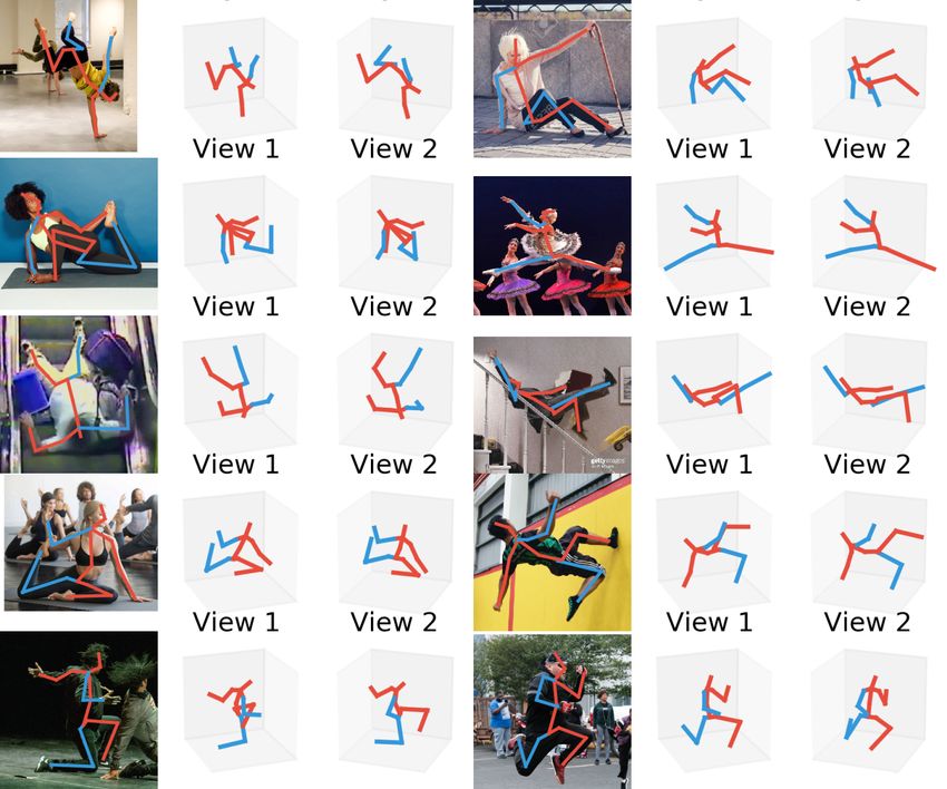
Head
ent descent basedPon a loss function defined over the train-
                    N                                                                             Nose
ing dataset L = i=1 E(pi , p̂i ) where E is the error mea-                                                    Neck
                                                                                      Right Shoulder            Left Shoulder                k
surement between the ground truth pi and the prediction                                                  Thorax
p̂i = F(φ(xi ), Θ).                                                                    Right Elbow         Spine                                 Parent
                                                                                                                       Left Elbow                    j
    Unfortunately, sampling bias exists during the data col-                                                  Pelvis
                                                                                       Right Wrist                                      i
lection and limits the variation of the training data. Hu-                                                                                       Bone
                                                                                                     Right Left        Left Wrist                Vector
man 3.6M (H36M) [22], the largest MC dataset, only con-                                              Hip   Hip
tains 11 subjects performing 15 actions under 4 viewpoints,                                Right Knee            Left Knee
leading to insufficient coverage of the training 2D-3D pairs                                                                                       Child
                                                                                              Right Foot
(φ(xi ), pi ). A DNN can overfit to the dataset bias and be-                                                       Left Foot

come less robust to unseen φ(x). For example, when a
subject starts street dancing, the DNN may fail since it is                         Figure 3: Hierarchical human representation. Left: 3D key-
only trained on daily activities such as sitting and walking.                       points organized in a kinematic tree where red arrows point
This problem is even exacerbated for the weakly-supervised                          from parent joints to children joints. Right: Zoom-in view
methods [48, 54, 12] where a minute quantity of training                            of a local coordinate system.
data is used to simulate the difficulty of data collection.
    We take a non-stationary view toward the training data to                                                              P
                                                                                     Mutation
cope with this problem. While conventionally the collected
training data is fixed and the trained DNN is not modified                           Crossover
during its deployment, here we assume the data and model
can evolve during their life-time. Specifically, we synthe-
size novel 2D-3D pairs based on an initial training dataset                                                                C
and add them into the original dataset to form the evolved                           P Parents
dataset. We then re-train the model with the evolved dataset.                        C Children
As shown in Fig. 2, model re-trained on the evolved dataset
has consistently lower generalization error, comparing to a
model trained on the initial dataset.                                               Figure 4: Examples of evolutionary operation. Crossover
                                                                                    and mutation take two and one random samples respectively
                           MPJPE (mm)                                               to synthesize novel human skeletons. In this example the
        113.1
 110                              Temporal convolution Pavllo et al. CVPR' 19       right arms are selected for crossover while the left leg is
        106.8                     Before evolution
                                  After evolution                                   mutated.
 100
        90.8
  90                                                                                Fig. 3. This representation captures the dependence of ad-
                        81.8
  80                    78.1
                        76.4
                                                                                    jacent joints with tree edges.
                                              72.5
                                                                                       Each 3D pose p corresponds to a set of bone vectors
                                              71.3                  71.0
  70                                                                                {b1 , b2 , · · · , bw } and a bone vector is defined as
                                              64.2                  65.2
                                                                    63.5
  %0.1 S1 (245)   %1 S1 (2.42k)       %5 S1 (12.4k)        %10 S1 (24.8k)                                    bi = pchild(i) − pparent(i)                     (1)
                          Training data
                                                                                    where pj is the jth joint in the 3D skeleton and parent(i)
Figure 2: Generalizing errors (MPJPE using ground truth
                                                                                    gives the parent joint index of the ith bone vector. A local
2D key-points as inputs) on H36M before and after dataset
                                                                                    coordinate system2 is attached at each parent node. For a
evolution with varying size of initial population.
                                                                                    parent node pparent(i) , its local coordinate system is repre-
                                                                                    sented by the rotation matrix defined by three basis vectors
   In the following we show that by using a hierarchical                            Ri = [ii , ji , ki ]. The global bone vector is transformed into
representation of human skeleton, the synthesis of novel                            this local coordinate system as
2D-3D pairs can be achieved by evolutionary operators and
                                                                                                         T                      T
camera projection.                                                                    bilocal = Ri biglobal = Ri (pchild(i) − pparent(i) ) (2)

3.1. Hierarchical Human Representation                                              For convenience, this local bone vector is further converted
                                                                                    into spherical coordinates bilocal = (ri , θi , φi ). The posture
   We represent a 3D human skeleton by a set of bones
organized hierarchically in a kinematic tree as shown in                              2 The   coordinate system is detailed in our supplementary material.

                                                                                3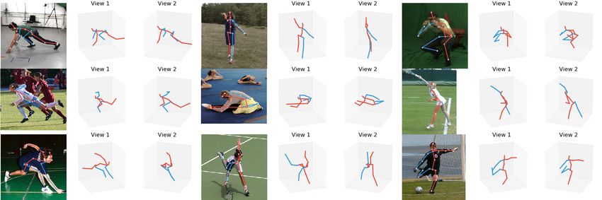
Algorithm 1 Data evolution                                                    skeleton may result in a valid new 3D pose. To implement
 Input:                                                                       this perturbation, our mutation operator modifies the local
 Initial set of 3D skeletons Dold = {pi }N
                                         i=1 , noise level σ, number of       orientation of one bone vector to get a new pose. One bone
generations G
 Output: Augmented set of skeletons Dnew = {pi }M
                                                                              vector bi = (ri , θi , φi ) for an input 3D pose is selected
                                                    i=1
 1: Dnew = Dold                                                               at random and its orientation is mutated by adding noise
 2: for i=1:G do                                                              (Gaussian in this study):
 3:      Parents = Sample(Dnew )
 4:      Children = NaturalSelection(Mutation(Crossover(Parents)))                                  θi0 = θi + gθ , φ0i = φi + gφ       (5)
 5:      Dnew = Dnew ∪ Children
 6: end for
 7: return Dnew                                                               where g ∼ N (0, σ) and σ is a pre-defined noise level. One
                                                                              example of mutating the left leg is shown in Fig. 4. We
                                                                              also mutate the global orientation and bone length of the 3D
of the skeleton is described by the collection of bone orien-                 skeletons to reduce the data bias of viewpoints and subject
tations {(θi , φi )}w
                    i=1 while the skeleton size is encoded into
                                                                              sizes, which is detailed in our supplementary material.
{ri }w
     i=1 .                                                                    Natural Selection We use a fitness function to evaluate the
                                                                              goodness of synthesized data for selection as v(p) which
3.2. Synthesizing New 2D-3D Pairs                                             indicates the validity of the new pose. v(p) can be any func-
   We first synthesize new 3D skeletons Dnew = {pj }M       j=1
                                                                              tion that describes how anatomically valid a skeleton is, and
with an initial training dataset Dold = {pi }N                                we implement it by utilizing the binary function in [2]. We
                                               i=1 and project
3D skeletons to 2D given camera intrinsics K to form 2D-                      specify v(p) = −∞ if p is not valid to rule out all invalid
3D pairs {(φ(xj ), pj )}M                                                     poses.
                           i=1 where φ(xj ) = Kpj .
   When adopting the hierarchical representation, a dataset                   Evolution Process The above operators are applied to Dold
of articulated 3D objects is a population of tree-structured                  to obtain a new generation Dnew by synthesizing new poses
data in nature. Evolutionary operators [20] have con-                         and merge with the old poses. This evolution process re-
structive property [62] that can be used to synthesize new                    peats G generations and is depicted in Algorithm 1. Finally,
data [16] given an initial population. The design of opera-                   Dnew are projected to 2D key-points to obtain paired 2D-
tors is problem-dependent and our operators are detailed as                   3D supervision.
follows.
Crossover Operator Given two parent 3D skeletons rep-                         4. Model Architecture
resented by two kinematic trees, crossover is defined as a                       We propose a two-stage model as shown in Fig. 5.
random exchange of sub-trees. This definition is inspired                     We name it TAG-Net, as the model’s focus transits from
by the observation that an unseen 3D pose might be ob-                        appearance to geometry. This model can be represented as
tained by assembling limbs from known poses. Formally,                        a function
we denote the set of bone vectors for parent A and B as
SA = {b1A , b2A , . . . , bw                 1    2         w
                           A } and SB = {bB , bB , . . . , bB }.                                     p̂ = TAG(x) = G(A(x))              (6)
A joint indexed by q is selected at random and the bones
rooted at it are located for the two parents. These bones                     Given an input RGB image x, A(x) (the appearance stage)
form the chosen sub-tree set Schosen                                          regresses k = 17 high-resolution probability heat-maps
                                                                              Hki=1 for k 2D human key-points and map them into 2D
        {bj : parent(j) = q ∨ IsOff (parent(j), q)}                (3)        coordinates c = (xi , yi )ki=1 . G(c) (the geometry stage) in-
                                                                              fers 3D key-point coordinates3 p = (xi , yi , zi )ki=1 in the
where IsOff (parent(j), q) is True if joint parent(j) is an
                                                                              camera coordinate system from input 2D coordinates. Key
offspring of joint q in the kinematic tree. The parent bones
                                                                              designs are detailed as follows.
are split into the chosen and the remaining ones as SX =
  X           X           X               X
Schosen  ∪ Srem  where Srem    = SX − Schosen    and X is A                   4.1. High-resolution Heatmap Regression
or B. Now the crossover operator gives two sets of children
bones as                                                                         Synthesized 2D key-points are projected from 3D points
                                                                              and can be thought as perfect detections while real detec-
       A         B                       B         A
 SC = Schosen ∪ Srem           and SD = Schosen ∪ Srem (4)                    tions produced by heat-map regression models are more
                                                                              noisy. We hope this noise can be small since we need to
These two new sets are converted into two new 3D skele-
                                                                              merge these two types of data as described in Section 3.
tons. The example in Fig. 4 shows the exchange of the right
                                                                              To detect 2D key-points as accurate as possible, we de-
arms when the right shoulder joint is selected.
                                                                              cide to obtain feature maps with high spatial resolution and
Mutation Operator As the motion of human limbs is usu-
ally continuous, a perturbation of one limb of an old 3D                        3 Relative   to the root joint.

                                                                          4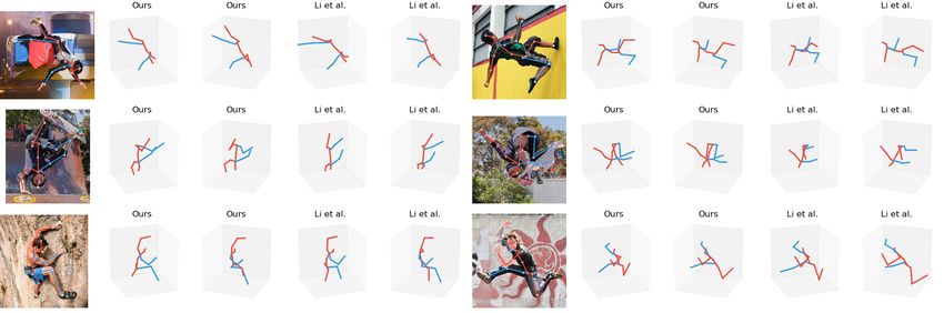
.   .   .
                                                                                                                              C                   .   .    .
                                                                                                                                                                                           +                  .   .   .

                                                                                                                                                                                                         Stage 2C...
                                                         2D
                                                         Joints                                                  3D                                                          Offsets
                                                                   3D Pose Regression Model (Stage 2A)           Joints        3D Pose Refinement Model (Stage 2B)
          Heatmap Regression Model
                 (Stage 1)

         Input/Output Coordinates
          3D Pose Representation                                                                  +                                        +                                           +         .   .    .

           Fully Connected Layer                                                                                                                                                               Later blocks
              Skip Connection        (1, 2*k)
                                                                                                                                                                                                                          (1, 3*k)
k: Number of human keypoints                    (1, d)            (1, d)   (1, d)                 (1, d)      (1, d)      (1, d)             (1, d)            (1, d)   (1, d)                            (1, d)
d: Representation dimension
                                                         Residual Block 1                                  Residual Block 2                               Residual Block 3

Figure 5: Our cascaded 3D pose estimation architecture. Top: our model is a two-stage model where the first stage is a 2D
landmark detector and the second stage is a cascaded 3D coordinate regression model. Bottom: each learner in the cascade
is a feed-forward neural network whose capacity can be adjusted by the number of residual blocks. To fit an evolved dataset
with plenty 2D-3D pairs, we use 8 layers (3 blocks) for each deep learner and have 24 layers in total with a cascade of 3 deep
learners.

use HR-Net [64] as our backbone for feature extraction.                                                                      the first learner D1 in the cascade directly predicts 3D co-
While the original model predicts heat-maps of size 96 by                                                                    ordinates while the later ones predict the 3D refinement
72, we append a pixel shuffle super-resolution layer [60]                                                                    δp = (δxi , δyi , δzi )ki=1 . While cascaded coordinate re-
to the end and regress heat-maps of size 384 by 288. The                                                                     gression has been adopted for 2D key-points localization
original model [64] uses hard arg-max to predict 2D co-                                                                      [10, 52], hand-crafted image feature and classical weak
ordinates, which results in rounding errors in our experi-                                                                   learners such as linear regressors were used. In contrast,
ments. Instead, we use soft arg-max [43, 65] to obtain 2D                                                                    our geometric model G(c) only uses coordinates as input
coordinates. The average 2D key-point localization errors                                                                    and each learner is a fully-connected (FC) DNN with resid-
for H36M testing images are shown in Tab. 1. Our design                                                                      ual connections [19].
choice improves the previous best model and achieves the                                                                         The bottom of Fig. 5 shows the detail for each deep
highest key-point localization accuracy on H36M to date.                                                                     learner. One deep learner first maps the input 2D coordi-
The extensions add negligible amount of parameters and                                                                       nates into a representation vector of dimension d = 1024,
computation.                                                                                                                 after which R = 3 residual blocks are used. Finally the
                                                                                                                             representation is mapped into 3D coordinates. After each
      Backbone           Extension         #Params                 FLOPs              Error↓
      CPN [13]               -                 -                   13.9G               5.40
                                                                                                                             FC layer we add batch normalization [21] and dropout [63]
      HRN [64]               -              63.6M                  32.9G            4.98↓7.8%                                with dropout rate 0.5. The capacity of each deep learner can
      HRN                  +U               63.6M                  32.9G            4.64↓14.1%                               be controlled by R. This cascaded model is trained sequen-
      HRN                 +U+S              63.6M                  32.9G            4.36↓19.2%                               tially by gradient descent and the training algorithm is in-
                                                                                                                             cluded in our supplementary material. Despite the number
Table 1: Average 2D key-point localization errors for H36M                                                                   of parameters increase linearly with the cascade length, we
testing set in terms of pixels. U: Heat-map up-sampling.                                                                     found that the cascaded model is robust to over-fitting for
S: use soft-argmax. Error reduction compared with the pre-                                                                   this 3D coordinate prediction problem, which is also shared
vious best model [13] used in [49] follows the ↓ signs.                                                                      by the 2D counterparts [10, 52].

4.2. Cascaded Deep 3D Coordinate Regression                                                                                  4.3. Implementation Details
   Since the mapping from 2D coordinates to 3D joints can                                                                        The camera intrinsics provided by H36M are used to
be highly-nonlinear and difficult to learn, we propose a cas-                                                                project 3D skeletons. We train A(x) and G(c) sequentially.
caded 3D coordinate regression model as                                                                                      The input size is 384 by 288 and our output heat-map has
                                                                                                                             the same high resolution. The back-bone of A(x) is pre-
                                                T
                                                X                                                                            trained on COCO [32] and we fine-tune it on H36M with
                         p̂ = G(c) =                     Dt (it , Θt )                                     (7)               Adam optimizer using a batch size of 24. The training is
                                                t=1
                                                                                                                             performed on two NVIDIA Titan Xp GPUs and takes 8
where Dt is the tth deep learner in the cascade parametrized                                                                 hours for 18k iterations. We first train with learning rate
by Θt and takes input it . As shown in the top of Fig. 5,                                                                    0.001 for 3k iterations, after which we multiply it by 0.1

                                                                                                                     5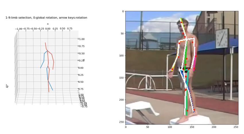
Figure 6: Cross-dataset inferences of G(c) on MPI-INF-3DHP (first row) and LSP (next two rows).

after every 3k iterations. To train G(c), we train each deep          MPI-INF-3DHP (3DHP) is a benchmark that we use
learner in the cascade using Adam optimizer with learning          to evaluate the generalization power of 2D-to-3D networks
rate 0.001 for 200 epochs.                                         in unseen environments. We do not use its training data
                                                                   and conduct cross-dataset inference by feeding the provided
5. Experiments                                                     key-points to G(c). Apart from MPJPE, Percentage of Cor-
                                                                   rect Keypoints (PCK) measures correctness of 3D joint pre-
    To validate our data evolution framework, we evolve
                                                                   dictions under a specified threshold, while Area Under the
from the training data provided in H36M and investigate
                                                                   Curve (AUC) is computed for a range of PCK thresholds.
how data augmentation may affect the generalization ability
of 2D-to-3D networks. We conduct both intra- and cross-               Unconstrained 3D Poses in the Wild (U3DPW) We
dataset evaluation. Intra-dataset evaluation is performed on       collect by ourselves a new small dataset consisting of 300
H36M and demonstrates the model performance in an in-              challenging in-the-wild images with rare human poses,
door environment similar to the training data. Cross-dataset       where 150 of them are selected from Leeds Sports Pose
evaluation is conducted on datasets not seen during training       dataset [23]. The annotation process is detailed in our sup-
to simulate a larger domain shift. Considering the avail-          plementary material. This dataset is used for qualitatively
ability of MC data may vary in different application sce-          validating model generalization for unseen rare poses.
narios, We vary the size of initial population starting from
                                                                   5.2. Comparison with state-of-the-art methods
scarce training data. These experiments help comparison
with other weakly/semi-supervised methods that only use            Comparison with weakly-supervised methods. Here we
very few 3D annotation but do not consider data augmen-            compare with weakly/semi-supervised methods, which only
tation. Finally we present an ablation study to analyze            use a small number of training data to simulate scarce data
the influences of architecture design and choice of hyper-         scenario. To be consistent with others, we utilize S1 as
parameters.                                                        our initial population. While others fix S1 as the training
                                                                   dataset, we evolve from it to obtain an augmented train-
5.1. Datasets and Evaluation Metrics
                                                                   ing set. The comparison of model performance is shown
    Human 3.6M (H36M) is the largest 3D human pose es-             in Tab. 2, where our model significantly out-performs oth-
timation benchmark with accurate 3D labels. We denote a            ers and demonstrates effective use of the limited training
collection of data by appending subject ID to S, e.g., S15         data. While other methods [54, 25] use multi-view consis-
denotes data from subject 1 and 5. Previous works fix the          tency as extra supervision, we achieve comparable perfor-
training data while our method uses it as our initial popu-        mance with only a single view by synthesizing useful su-
lation and evolves from it. We evaluate model performance          pervision. Fig. 2 validates our method when the training
with Mean Per Joint Position Error (MPJPE) measured in             data is extremely scarce, where we start with a small frac-
millimeters. Two standard evaluation protocols are adopted.        tion of S1 and increase the data size by 2.5 times by evolu-
Protocol 1 (P1) directly computes MPJPE while Protocol 2           tion. Note that the model performs consistently better after
(P2) aligns the ground-truth 3D poses with the predictions         dataset evolution. Compared to the temporal convolution
with a rigid transformation before calculating it. Protocol        model proposed in [49], we do not utilize any temporal in-
P1∗ uses ground truth 2D key-points as inputs and removes          formation and achieve comparable performance. This indi-
the influence of the first stage model.                            cates our approach can make better use of extremely limited

                                                               6
data.
                                            Average MPJPE↓
             Method (Reference)
                                           P1     P1*    P2
                         Use Multi-view Images
        Rhodin et al. (CVPR’18) [54]        -      -    64.6
        Kocabas et al. (CVPR’19) [25]     65.3     -    57.2
                Use Temporal Information from Videos
         Pavllo et al. (CVPR’19) [49]     64.7     -      -
                        Use a Single RGB Image
           Li et al. (ICCV’19) [30]       88.8     -    66.5
              Ours (CVPR’ 20)             60.8    50.5  46.2        Figure 7: Dataset distribution for the bone vector connect-
                                                                    ing right shoulder to right elbow. Top: distribution before
Table 2: Comparison with SOTA weakly-supervised meth-               (left) and after (right) dataset augmentation. Bottom: distri-
ods. Average MPJPE over all 15 actions for H36M under               bution overlaid with valid regions (brown) taken from [2].
two protocols (P1 and P2) is reported. P1* refers to proto-
col 1 evaluated with ground truth 2d key-points. Best per-
formance is marked with bold font. Error for each action            these unconstrained poses are not well-represented in the
can be found in Tab. 7.                                             original training dataset yet our model still gives good in-
                                                                    ference results. Qualitative comparison with [28] on some
Comparison with fully-supervised methods. Here we                   difficult poses in U3DPW is shown in Fig. 8 and our G(c)
compare with fully-supervised methods that uses the whole           generalizes better for these rare human poses.
training split of H36M. We use S15678 as our initial popu-                Method              CE   PCK↑    AUC↑    MPJPE↓
lation and Tab. 3 shows the performance comparison. Un-                   Mehta et al. [38]         76.5    40.8    117.6
der this setting, our model also achieves competitive perfor-             VNect [40]                76.6    40.4    124.7
mance compared with other SOTA methods, indicating that                   LCR-Net [56]              59.6    27.6    158.4
                                                                          Zhou et al. [74]          69.2    32.5    137.1
our approach is not limited to scarce data scenario.                      Multi Person [39]         75.2    37.8    122.2
                                                                          OriNet [35]               81.8    45.2    89.4
                                           Average MPJPE↓                 Li et al. [28]      X     67.9     -        -
             Method (Reference)
                                          P1     P1*    P2                Kanazawa [24]       X     77.1    40.7    113.2
        Martinez et al. (ICCV’17) [37]   62.9    45.5  47.7               Yang et al. [71]    X     69.0    32.0      -
         Yang et al. (CVPR’18) [71]      58.6     -    37.7               Ours                X     81.2    46.1    99.7
         Zhao et al. (CVPR’19) [73]      57.6    43.8    -
        Sharma et al. (ICCV’19) [58]     58.0     -    40.9
         Moon et al. (ICCV’19) [41]      54.4    35.2    -
                                                                    Table 4: Testing results for the MPI-INF-3DHP dataset.
              Ours (CVPR’ 20)            50.9    34.5  38.0         A higher value is better for PCK and AUC while a lower
                                                                    value is better for MPJPE. MPJPE is evaluated without rigid
Table 3: Comparison with SOTA methods under fully-                  transformation. CE denotes cross-dataset evaluation and the
supervised setting. Same P1, P1* and P2 as in Tab. 2. Error         training data in MPI-INF-3DHP is not used.
for each action can be found in Tab. 6.

                                                                    5.4. Ablation Study
5.3. Cross-dataset Generalization
                                                                    Effect of data evolution. Our ablation study is conducted
    To validate the generalization ability of our 2D-to-3D          on H36M and summarized in Tab. 5. The baseline (B) uses
network in unknown environment, Tab. 4 compares with                T =1. Note that adding cascade (B+C) and dataset evolution
other methods on 3DHP. In this experiment we evolve from            (B+C+E) consistently out-performs the baseline. Discus-
S15678 in H36M to obtain an augmented dataset consist-              sion on the evolution operators is included in our supple-
ing of 8 million 2D-3D pairs. Without utilizing any train-          mentary material.
ing data of 3DHP, G(c) achieves competitive performance             Effect of cascade length T. Here we train our model on var-
in this benchmark. We obtain clear improvements compar-             ious subsets of H36M and plot MPJPE over cascade length
ing with [28], which also uses S15678 as the training data          as shown in Fig. 9. Here R is fixed as 2. Note that the
but fix it without data augmentation. The results indicate          training error increases as the training set becomes more
that our data augmentation approach improves model gen-             complex and the testing errors decreases accordingly. The
eralization effectively despite we start with the same biased       gap between these two errors indicate insufficient training
training dataset. As shown in Fig. 7, the distribution of the       data. Note that with increasing number of deep learners,
augmented dataset indicates less dataset bias. Qualitative          the training error is effectively reduced but the model does
results on 3DHP and LSP are shown in Fig. 6. Note that              not overfit. This property is brought by the ensemble effect

                                                                7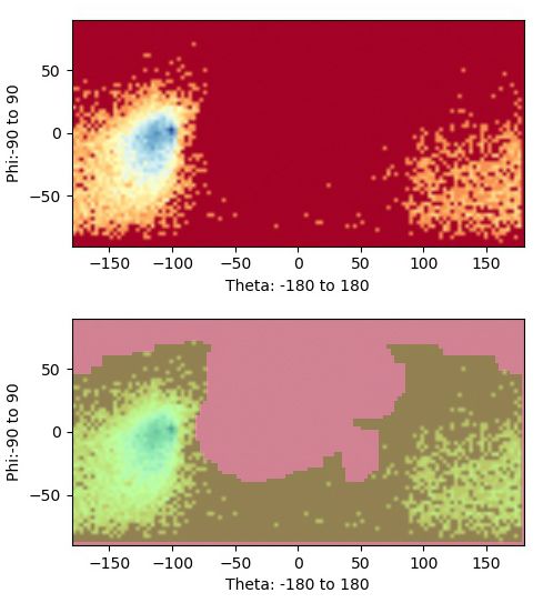
Figure 8: Cross-dataset inference results on U3DPW comparing with [28]. Video is included in our supplementary material.

                                                                                          MPJPE (mm) under P1*
of multiple deep learners.                                                 20        Train: BE
Effect of block number R. Here we fix T =1, d=512 and                                Test: BE
vary R. S15678 in H36M and its evolved version are used.                   10        Train: AE
The datasets before (BE) and after evolution (AE) are ran-                           Test: AE
domly split into training and testing subsets for simplicity.
                                                                            0                          1   3     5    7     9
The training and testing MPJPEs are shown in Fig. 10. Note
that the training error is larger after evolution with the same                             Number of blocks R
R=7. This means our approach increases the variation of               Figure 10: MPJPE (P1*) before (BE) and after evolution
training data, which can afford a deeper architecture with            (AE) with varying number of blocks R. Evolved training
larger R (e.g. R=9).                                                  data can afford a deeper network. Best viewed in color.
                  Training MPJPE (mm) under P1*                                                                   MPJPE
    20                                                 S1                   Method     Training Data
                                                                                                             P1            P1*
                                                       S15                     Problem Setting A: Weakly-supervised Learning
                                                       S156
    10                                                                      B               S1              71.5          66.2
         1                   2                     3
                                                                            B+C             S1            70.1↓2.0%     64.5↓2.6%
                                                                            B+C+E       Evolve(S1)       60.8↓15.0%    50.5↓21.7%
                  Testing MPJPE (mm) under P1*                                  Problem Setting B: Fully-supervised Learning
         66.1                 64.5                 64.1                     B             S15678            54.3          44.5
    60   60.8                 59.9                 60.0                     B+C           S15678          52.1↓4.0%     42.9↓3.6%
                                                                            B+C+E     Evolve(S15678)      50.9↓6.2%    34.5↓22.4%
    50   49.4                 48.6                 48.5
         1                    2                    3                  Table 5: Ablation study on H36M. B: baseline. C: add cas-
                         Cascade length                               cade. E: add data evolution. Evolve() represents the data
Figure 9: Training and testing errors with varying number             augmentation operation. Same P1 and P1* as in Table 2.
of cascade length and training data. S156 indicates using             Error reduction compared with the baseline follows the ↓
3D annotations from subjects 1, 5 and 6. The cascade effec-           signs.
tively reduces training error and is robust to over-fitting.

                                                                      mation. There are many fruitful directions remaining to be
                                                                      explored. Extension to temporal domain, multi-view setting
6. Conclusion                                                         and multi-person scenarios are three examples. In addition,
   This paper presents an evolutionary framework to enrich            instead of being fixed, the operators can also evolve during
the 3D pose distribution of an initial biased training set.           the data generation process.
This approach leads to better intra-dataset and cross-dataset         Acknowledgments We gratefully acknowledge the support
generalization of 2D-to-3D network especially when avail-             of NVIDIA Corporation with the donation of one Titan Xp
able 3D annotation is scarce. A novel cascaded 3D hu-                 GPU used for this research. This research is also supported
man pose estimation model is trained achieving state-of-              in part by Tencent and the Research Grant Council of the
the-art performance for single-frame 3D human pose esti-              Hong Kong SAR under grant no. 1620818.

                                                                  8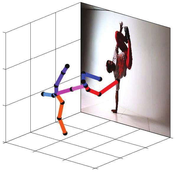
Supplementary Material                                  Algorithm 2 Computation of local bone vector
                                                                       Input: ith global bone vector bg = biglobal , constant 3D vector a
   This supplementary material includes implementation                 Output: ith local bone vector bl = bilocal with its local coordinate
details and extended experimental analysis that are not in-           system Ri
cluded in the main text due to space limit. The detailed               1: backBone = Spine - Thorax
MPJPE under different settings are shown Tab. 6 and Tab. 7.            2: if bg is upper limb then
                                                                       3:     v1 = rightShoulder - leftShoulder
Other contents are organized in separate sections as follows:          4:     v2 = backBone
                                                                       5: else if bg is lower limb then
   • Section 7 includes the implementation details of the              6:     v1 = rightHip - leftHip
     hierarchal human representation.                                  7:     v2 = backBone
                                                                       8: else
                                                                                      M (i)
   • Section 8 elaborates the model training, which in-                9:     v1 = bg
     cludes the training algorithm of the cascaded model              10:      v2 = RM (i) a × v1
                                                                      11: end if
     and describes details of data pre-processing.                    12: Ri = GramSchmidt(v1 , v2 , v1 × v2 )
                                                                                    T
                                                                      13: bl = Ri bg
   • Section 9 gives ablation study on data generation and            14: return bl
     the evolutionary operators.

   • Section 10 describes the new dataset U3DPW and its
                                                                      7.2. Validity Function
     collection process.
                                                                          To implement v(p), local bone vectors are first computed
                                                                      by Algorithm 2 and converted into spherical coordinates as
7. Hierarchical Human Model                                           bilocal = (ri , θi , φi ). A pose p is then considered as the
                                                                                                                w
7.1. Choice of Local Coordinate System                                collection of bone orientations (θi , φi )i=1 . A function is
                                                                      provided by [2] to decide the validity of each tuple (θi , φi ).
    As mentioned at equation 2 in section 3.1, each global            We define a pose p to be anthropometrically valid if every
bone vector is transformed into a local bone vector with              tuple (θi , φi ) is valid:
respect to a coordinate system attached at a parent joint.
In general, the choice of the coordinate system is arbitrary                      (
and our evolutionary operators do not depend on it. In im-                         0,          if (θi , φi ) is valid for i=1,2,...,w,
                                                                           v(p) =
plementation, we adopt the coordinate system proposed in                           −∞,         else.
[2], where the computation of basis vectors depends on the
3D joint position. For the bone vectors representing upper            The original code released by [2] was implemented by
limbs (left shoulder to left elbow, right shoulder to right el-       MATLAB and we provide a Python implementation on our
bow, left hip to left knee, right hip to right knee), the basis       project website.
vectors are computed based on several joints belonging to
the human torso. For the bone vectors representing lower              8. Model Training
limbs (left elbow to left wrist, right elbow to right wrist,          8.1. Training Procedure of the Cascaded Model
left knee to left ankle, right knee to right ankle), the basis
vectors are computed from the parent bone vectors.                        We train each deep learner in the cascade sequentially as
    Algorithm 2 is adapted from [2] and details the pro-              depicted by algorithm 3. The T rainN etwork is a routine
cess of computing basis vectors and performing coordi-                representing the training process of a single deep learner,
nate transformation. Bold name such as rightShoulder de-              which consists of forward pass, backward pass and network
notes the global position of the 3D skeleton joint. We de-            parameter update using Adam optimizer. Starting from the
fine a bone vector’s parent bone vector as the bone vec-              second deep learner, the inputs can also be concatenated
tor whose end point is the starting point of it. An in-               with the current estimates as {φ(xi ), p̂i }N
                                                                                                                  i=1 , which results
dex mapping function M (i) is introduced here that maps               in slightly smaller training errors while the change of testing
bone vector index i to the index of its parent bone vec-              errors is not obvious in our experiments on H36M.
tor. Consistent with the notations of the main text, we have
                                                                      8.2. Data Pre-processing
child(M (i)) = parent(i). In implementation, we found
that the joints used in [2] have slightly different semantic              To train the heatmap regression model A(x), we down-
meaning compared to the data provided by H36M. Thus we                load training videos from the official website of H36M. We
use the bone vector connecting the spine and thorax joints to         crop the persons with the provided bounding boxes and pad
approximate the backbone vector used in in [2] (backBone              the cropped images with zeros in order to fix the aspect ra-
in algorithm 2).                                                      tio as 4:3. We then resize the padded images to 384 by 288.

                                                                  9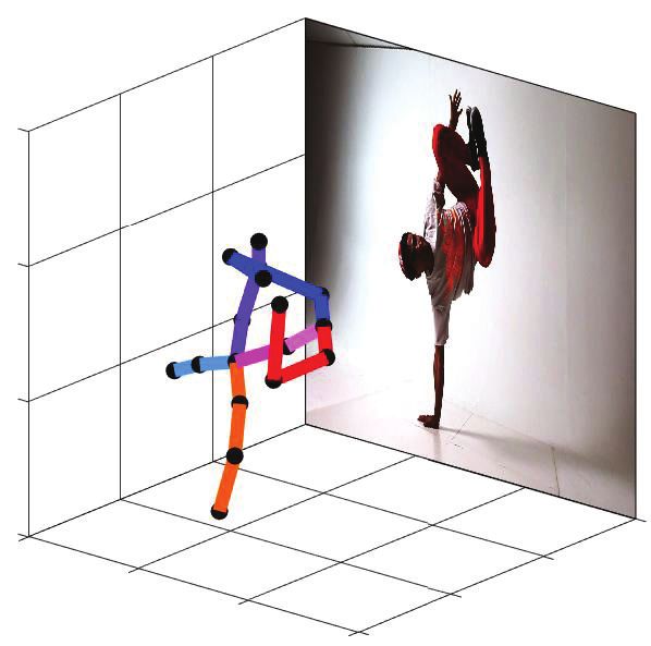
Protocol #1                      Dir.   Disc    Eat   Greet   Phone   Photo   Pose     Purch.    Sit    SitD.   Smoke   Wait   WalkD.   Walk   WalkT.   Avg.
Martinez et al. (ICCV’17)[37]    51.8   56.2   58.1    59.0    69.5    78.4    55.2     58.1     74.0   94.6    62.3    59.1    65.1    49.5    52.4    62.9
Fang et al. (AAAI’18) [17]       50.1   54.3   57.0    57.1    66.6    73.3    53.4     55.7     72.8   88.6    60.3    57.7    62.7    47.5    50.6    60.4
Yang et al. (CVPR’18) [71]       51.5   58.9   50.4    57.0    62.1    65.4    49.8     52.7     69.2   85.2    57.4    58.4    43.6    60.1    47.7    58.6
Pavlakos et al. (CVPR’18) [46]   48.5   54.4   54.4    52.0    59.4    65.3    49.9     52.9     65.8   71.1    56.6    52.9    60.9    44.7    47.8    56.2
Lee et al. (ECCV’18) [27]        40.2   49.2   47.8    52.6    50.1    75.0    50.2     43.0     55.8   73.9    54.1    55.6    58.2    43.3    43.3    52.8
Zhao et al. (CVPR’19) [73]       47.3   60.7   51.4    60.5    61.1    49.9    47.3     68.1     86.2   55.0    67.8    61.0    42.1    60.6    45.3    57.6
Sharma et al. (ICCV’19) [59]     48.6   54.5   54.2    55.7    62.6    72.0    50.5     54.3     70.0   78.3    58.1    55.4    61.4    45.2    49.7    58.0
Moon et al. (ICCV’19) [41]       51.5   56.8   51.2    52.2    55.2    47.7    50.9     63.3     69.9   54.2    57.4    50.4    42.5    57.5    47.7    54.4
Liu et al. (ECCV’20) [33]        46.3   52.2   47.3    50.7    55.5    67.1    49.2     46.0     60.4   71.1    51.5    50.1    54.5    40.3    43.7    52.4
Ours: Evolve(S15678)             47.0   47.1   49.3    50.5    53.9    58.5    48.8     45.5     55.2   68.6    50.8    47.5    53.6    42.3    45.6    50.9
Protocol #2                      Dir.   Disc    Eat   Greet   Phone   Photo   Pose     Purch.    Sit    SitD.   Smoke   Wait   WalkD.   Walk   WalkT.   Avg.
Martinez et al. (ICCV’17) [37]   39.5   43.2   46.4    47.0    51.0    56.0    41.4     40.6     56.5   69.4    49.2    45.0    49.5    38.0    43.1    47.7
Fang et al. (AAAI’18) [17]       38.2   41.7   43.7    44.9    48.5    55.3    40.2     38.2     54.5   64.4    47.2    44.3    47.3    36.7    41.7    45.7
Pavlakos et al. (CVPR’18) [46]   34.7   39.8   41.8    38.6    42.5    47.5    38.0     36.6     50.7   56.8    42.6    39.6    43.9    32.1    36.5    41.8
Yang et al. (CVPR’18) [71]       26.9   30.9   36.3    39.9    43.9    47.4    28.8     29.4     36.9   58.4    41.5    30.5    29.5    42.5    32.2    37.7
Sharma et al. (ICCV’19) [59]     35.3   35.9   45.8    42.0    40.9    52.6    36.9     35.8     43.5   51.9    44.3    38.8    45.5    29.4    34.3    40.9
Cai et al. (ICCV’19) [9]         35.7   37.8   36.9    40.7    39.6    45.2    37.4     34.5     46.9   50.1    40.5    36.1    41.0    29.6    33.2    39.0
Liu et al. (ECCV’20) [33]        35.9   40.0   38.0    41.5    42.5    51.4    37.8     36.0     48.6   56.6    41.8    38.3    42.7    31.7    36.2    41.2
Ours: Evolve(S15678)             34.5   34.9   37.6    39.6    38.8    45.9    34.8     33.0     40.8   51.6    38.0    35.7    40.2    30.2    34.8    38.0

Table 6: Quantitative comparisons with the state-of-the-art fully-supervised methods on Human3.6M under protocol #1 and
protocol #2. Best performance is indicated by bold font.

Protocol #1                      Dir.   Disc   Eat    Greet   Phone   Photo   Pose    Purch.     Sit    SitD.   Smoke   Wait   WalkD.   Walk   WalkT.   Avg.
Kocabas et al. (CVPR’19) [25]     -      -      -      -       -        -      -         -        -       -       -      -       -       -       -      65.3
Pavllo et al. (CVPR’19) [49]      -      -      -      -       -        -      -         -        -       -       -      -       -       -       -      64.7
Li et al. (ICCV’19) [30]         70.4   83.6   76.6   78.0    85.4    106.1   72.2     103.0    115.8   165.0    82.4   74.3    94.6    60.1    70.6    88.8
Ours: Evolve(S1)                 52.8   56.6   54.0   57.5    62.8    72.0    55.0     61.3     65.8    80.7     59.0   56.7    69.7    51.6    57.2    60.8
Protocol #2                      Dir.   Disc   Eat    Greet   Phone   Photo   Pose    Purch.     Sit    SitD.   Smoke   Wait   WalkD.   Walk   WalkT.   Avg.
Rhodin et al. (CVPR’18) [54]      -      -      -       -       -       -      -         -        -       -       -      -       -       -       -      64.6
Kocabas et al. (CVPR’19) [25]     -      -      -       -       -       -      -         -        -       -       -      -       -       -       -      57.2
Li et al. (ICCV’19) [30]          -      -      -       -       -       -      -         -        -       -       -      -       -       -       -      66.5
Ours: Evolve(S1)                 40.1   43.4   41.9   46.1    48.2    55.1    42.8     42.6     49.6    61.1     44.5   43.2    51.5    38.0    44.4    46.2

Table 7: Quantitative comparisons with the state-of-the-art weakly/semi-supervised methods on Human3.6M under protocol
#1 and protocol #2. Best performance is indicated by bold font.

Algorithm 3 Cascaded Deep Networks Training                                          8 pixels.
 Input:                                                                                 To train the cascaded 3D pose estimation model G(c)
 Training set {φ(xi ), pi }N
                           i=1 , cascade length T                                    on H36M, we download the pre-processed human skeletons
 Output: G(c) = T
                   P
                           D
                      t=1 t (it , Θt )                                               released by the authors of [37] in their github repository.
 1: Current estimate {p̂i }N
                           i=1 = 0
 2: Cascade G(c) = 0
                                                                                     Each deep learner in the cascaded model is trained with
 3: for t=1:T do                                                                     L2 loss. The evaluation set MPI-INF-3DHP is downloaded
 4:     Inputs it = {φ(xi )}Ni=1                                                     from the official website and we use the provided 2D key-
 5:     Regression targets = {pi − p̂i }Ni=1                                         points as inputs to evaluate the trained cascaded 2D-to-3D
 6:     Dt = T rainN etwork(Inputs, Regression targets)
 7:     G(c) = G(c) + Dt
                                                                                     model, which is consistent with and comparable to recent
 8:     for i=1:N do                                                                 works [28, 15].
 9:         p̂i = p̂i + Dt (φ(xi ))
10:     end for
11: end for
                                                                                     9. Ablation Study on Data Evolution
12: return G(c)
                                                                                     9.1. Effect of Number of Generation G
                                                                                        To study how the model performance improves with in-
The target heatmaps have the same size as the input im-                              creasing number of synthetic data, we start with S1 data in
ages and we draw a Gaussian dot for each human key-point                             Human 3.6M and synthesize training datasets with different
φ(x)ki=1 . The Gaussian dot’s mean is the ground truth 2D                            size by varying the number of generations G. We train one
location of the key-point and it has a standard deviation of                         model for each evolved dataset. All models have the save

                                                                              10
Figure 12: Training and testing errors under P1* with and
without adding mutation. C: crossover, M: mutation. Us-
ing crossover and mutation together out-performs using
crossover alone in our experiments.
Figure 11: Training and testing MPJPE under P1* with
varying number of generation (amount of training 2D-3D
pairs). 10.1. Image Selection
We start by collecting 300 in-the-wild images that con-
tain humans whose pose is not constrained to daily actions.
architecture and in this study where we fix T =1 and R=2.
We select 150 images from the existing LSP dataset [23]
These models’ performance (MPJPE under P1*) are shown
and the remaining 150 high-resolution images are gathered
in Fig. 11. Number of generations and the corresponding
from the Internet. To choose from the LSP dataset, we run
number of 2D-3D pairs are indicated on the x-axis by (G,
SMPLify [7] on all available images and manually select
N). We observe that the testing errors decrease steadily with
150 images with large fitting errors.
larger G (more synthetic data) while the training errors have
the opposite trend. This indicates that our data evolution ap- 10.2. 2D Annotation
proach indeed synthesizes novel supervision to augment the
original dataset. The changing performance of the model We annotate 17 semantic 2D key-points for each image
can be seen as it is evolving along with the growing train- in U3DPW. These key-points are: right ankle, right knee,
ing dataset, where the model generalization power is signif- right hip, left hip, left knee, left ankle, right wrist, right
icantly improved. elbow, right shoulder, left shoulder, left elbow, left wrist,
neck, head top, spine, thorax and nose. Example new im-
9.2. Effect of Evolutionary Operators ages (not in LSP) with 2D annotations are shown in Fig. 15.
These images include large variation of human poses, cam-
There has been debates on the individual function of
era viewpoints and illumination. Although we focus on 3D
crossover and mutation operators [62]. In [62] the au-
pose estimation in this work, these 2D annotations can also
thor shows theoretically that the mutation operator has
be used to evaluate 2D pose estimation models for uncon-
stronger disruptive property while the crossover operator
strained scenarios.
has stronger constructive property. Here we conduct em-
pirical experiments to study the effectiveness of these evo- 10.3. 3D Annotation
lutionary operators applied on our problem. Here we com-
pare between data evolution with crossover along and us- Using a subset of 2D key-points we run SMPLify [7] to
ing both operators. The same initial population and model obtain fitted 3D human poses.
hyper-parameters as in Section 9.1 are adopted. The train- We provide an annotation tools that can be used after
ing and testing MPJPEs are shown in Fig. 12. We observe running SMPLify. The annotation tool displays the 3D
that adding mutation (+M) slightly increases training errors skeleton after SMPLify fitting, current image and the pro-
but decreases testing errors just like adding more data in jected 2D key-points (calculated with the camera intrinsics
Section 9.1. Despite the difference is not huge, this indi- from the SMPLify fitting results). The fitted skeleton is con-
cates that using both operators is beneficial for our problem. verted into a hierarchical human representation, and the user
can interactively modify the global pose orientation and the
local bone vector orientation by keyboard inputs. With the
10. Details for U3DPW user feeding inputs, new positions of the 2D human key-
points are updated in real-time so that the user can align
In this section, we describe how we collect and annotate the 2D projections with some reference key-points. One
the images for our new dataset U3DPW. video demo of operating the annotation tool is placed at
11Figure 13: 3D annotation examples for U3DPW shown in two different viewpoints.
11. Others
11.1. Video for Qualitative Comparison
The qualitative comparison with [28] (Fig. 8) is included
as video for better visualization. The file can be found at
root/videos/annotation/qualitative.mkv
11.2. Failure Cases
Some individual cases are included as videos in root/
videos/. Projection ambiguity is hard to resolve in some
Figure 14: A snapshot of the annotation process. Left: 3D
cases and image features should be incorporated instead of
human skeleton. Right: image and 2D projections.
only using key-points as inputs.
root/videos/annotation_tool.mkv. Here root
refers to the directory of the unzipped supplementary ma-
terial folder. Some exemplar 3D annotations are shown in
Fig. 13.
12Figure 15: Exemplar images of U3DPW with 2D annotations.
13References Conference on Computer Vision and Pattern Recognition,
pages 7103–7112, 2018. 5
[1] Ankur Agarwal and Bill Triggs. Recovering 3d human pose [14] Yu Cheng, Bo Yang, Bo Wang, Wending Yan, and Robby T.
from monocular images. IEEE transactions on pattern anal- Tan. Occlusion-aware networks for 3d human pose estima-
ysis and machine intelligence, 28(1):44–58, 2005. 2 tion in video. In The IEEE International Conference on
[2] Ijaz Akhter and Michael J Black. Pose-conditioned joint an- Computer Vision (ICCV), October 2019. 1
gle limits for 3d human pose reconstruction. In Proceed- [15] Hai Ci, Chunyu Wang, Xiaoxuan Ma, and Yizhou Wang. Op-
ings of the IEEE conference on computer vision and pattern timizing network structure for 3d human pose estimation.
recognition, pages 1446–1455, 2015. 2, 4, 7, 9 In The IEEE International Conference on Computer Vision
[3] Mykhaylo Andriluka, Leonid Pishchulin, Peter Gehler, and (ICCV), October 2019. 1, 10
Bernt Schiele. 2d human pose estimation: New benchmark [16] João Correia, Tiago Martins, and Penousal Machado. Evo-
and state of the art analysis. In IEEE Conference on Com- lutionary data augmentation in deep face detection. In Pro-
puter Vision and Pattern Recognition (CVPR), June 2014. 2 ceedings of the Genetic and Evolutionary Computation Con-
[4] Dragomir Anguelov, Praveen Srinivasan, Daphne Koller, Se- ference Companion, pages 163–164, 2019. 4
bastian Thrun, Jim Rodgers, and James Davis. Scape: shape [17] Hao-Shu Fang, Yuanlu Xu, Wenguan Wang, Xiaobai Liu,
completion and animation of people. In ACM transactions on and Song-Chun Zhu. Learning pose grammar to encode hu-
graphics (TOG), volume 24, pages 408–416. ACM, 2005. 2 man body configuration for 3d pose estimation. In Thirty-
[5] Vasileios Belagiannis, Sikandar Amin, Mykhaylo Andriluka, Second AAAI Conference on Artificial Intelligence, 2018. 10
Bernt Schiele, Nassir Navab, and Slobodan Ilic. 3d pictorial [18] Ikhsanul Habibie, Weipeng Xu, Dushyant Mehta, Gerard
structures for multiple human pose estimation. In Proceed- Pons-Moll, and Christian Theobalt. In the wild human pose
ings of the IEEE Conference on Computer Vision and Pattern estimation using explicit 2d features and intermediate 3d
Recognition, pages 1669–1676, 2014. 2 representations. In Proceedings of the IEEE Conference
[6] Liefeng Bo and Cristian Sminchisescu. Structured output- on Computer Vision and Pattern Recognition, pages 10905–
associative regression. In 2009 IEEE Conference on Com- 10914, 2019. 2
puter Vision and Pattern Recognition, pages 2403–2410. [19] Kaiming He, Xiangyu Zhang, Shaoqing Ren, and Jian Sun.
IEEE, 2009. 2 Deep residual learning for image recognition. In Proceed-
[7] Federica Bogo, Angjoo Kanazawa, Christoph Lassner, Peter ings of the IEEE conference on computer vision and pattern
Gehler, Javier Romero, and Michael J Black. Keep it smpl: recognition, pages 770–778, 2016. 5
Automatic estimation of 3d human pose and shape from a [20] John Henry Holland et al. Adaptation in natural and arti-
single image. In European Conference on Computer Vision, ficial systems: an introductory analysis with applications to
pages 561–578. Springer, 2016. 2, 11 biology, control, and artificial intelligence. MIT press, 1992.
[8] Magnus Burenius, Josephine Sullivan, and Stefan Carlsson. 4
3d pictorial structures for multiple view articulated pose esti- [21] Sergey Ioffe and Christian Szegedy. Batch normalization:
mation. In Proceedings of the IEEE Conference on Computer Accelerating deep network training by reducing internal co-
Vision and Pattern Recognition, pages 3618–3625, 2013. 2 variate shift. arXiv preprint arXiv:1502.03167, 2015. 5
[9] Yujun Cai, Liuhao Ge, Jun Liu, Jianfei Cai, Tat-Jen Cham, [22] Catalin Ionescu, Dragos Papava, Vlad Olaru, and Cristian
Junsong Yuan, and Nadia Magnenat Thalmann. Exploit- Sminchisescu. Human3. 6m: Large scale datasets and pre-
ing spatial-temporal relationships for 3d pose estimation dictive methods for 3d human sensing in natural environ-
via graph convolutional networks. In Proceedings of the ments. IEEE transactions on pattern analysis and machine
IEEE/CVF International Conference on Computer Vision, intelligence, 36(7):1325–1339, 2013. 1, 2, 3
pages 2272–2281, 2019. 10 [23] Sam Johnson and Mark Everingham. Clustered pose and
[10] Xudong Cao, Yichen Wei, Fang Wen, and Jian Sun. Face nonlinear appearance models for human pose estimation. In
alignment by explicit shape regression. International Jour- Proceedings of the British Machine Vision Conference, 2010.
nal of Computer Vision, 107(2):177–190, 2014. 5 doi:10.5244/C.24.12. 6, 11
[11] Wenzheng Chen, Huan Wang, Yangyan Li, Hao Su, Zhen- [24] Angjoo Kanazawa, Michael J Black, David W Jacobs, and
hua Wang, Changhe Tu, Dani Lischinski, Daniel Cohen- Jitendra Malik. End-to-end recovery of human shape and
Or, and Baoquan Chen. Synthesizing training images for pose. In Proceedings of the IEEE Conference on Computer
boosting human 3d pose estimation. In 2016 Fourth Inter- Vision and Pattern Recognition, pages 7122–7131, 2018. 7
national Conference on 3D Vision (3DV), pages 479–488. [25] Muhammed Kocabas, Salih Karagoz, and Emre Akbas. Self-
IEEE, 2016. 2 supervised learning of 3d human pose using multi-view ge-
[12] Xipeng Chen, Kwan-Yee Lin, Wentao Liu, Chen Qian, and ometry. In Proceedings of the IEEE Conference on Computer
Liang Lin. Weakly-supervised discovery of geometry-aware Vision and Pattern Recognition, pages 1077–1086, 2019. 2,
representation for 3d human pose estimation. In Proceed- 6, 7, 10
ings of the IEEE Conference on Computer Vision and Pattern [26] Nikos Kolotouros, Georgios Pavlakos, Michael J. Black, and
Recognition, pages 10895–10904, 2019. 2, 3 Kostas Daniilidis. Learning to reconstruct 3d human pose
[13] Yilun Chen, Zhicheng Wang, Yuxiang Peng, Zhiqiang and shape via model-fitting in the loop. In The IEEE Inter-
Zhang, Gang Yu, and Jian Sun. Cascaded pyramid network national Conference on Computer Vision (ICCV), October
for multi-person pose estimation. In Proceedings of the IEEE 2019. 2
14[27] Kyoungoh Lee, Inwoong Lee, and Sanghoon Lee. Propagat- Conference on 3D Vision (3DV), pages 120–130. IEEE,
ing lstm: 3d pose estimation based on joint interdependency. 2018. 7
In Proceedings of the European Conference on Computer Vi- [40] Dushyant Mehta, Srinath Sridhar, Oleksandr Sotnychenko,
sion (ECCV), pages 119–135, 2018. 10 Helge Rhodin, Mohammad Shafiei, Hans-Peter Seidel,
[28] Chen Li and Gim Hee Lee. Generating multiple hypotheses Weipeng Xu, Dan Casas, and Christian Theobalt. Vnect:
for 3d human pose estimation with mixture density network. Real-time 3d human pose estimation with a single rgb cam-
In Proceedings of the IEEE Conference on Computer Vision era. ACM Transactions on Graphics (TOG), 36(4):44, 2017.
and Pattern Recognition, pages 9887–9895, 2019. 1, 2, 7, 8, 7
10, 12 [41] Gyeongsik Moon, Juyong Chang, and Kyoung Mu Lee.
[29] Yi Li and Nuno Vasconcelos. Repair: Removing representa- Camera distance-aware top-down approach for 3d multi-
tion bias by dataset resampling. In Proceedings of the IEEE person pose estimation from a single rgb image. In The IEEE
Conference on Computer Vision and Pattern Recognition, Conference on International Conference on Computer Vision
pages 9572–9581, 2019. 2 (ICCV), 2019. 7, 10
[30] Zhi Li, Xuan Wang, Fei Wang, and Peilin Jiang. On boost- [42] Francesc Moreno-Noguer. 3d human pose estimation from
ing single-frame 3d human pose estimation via monocular a single image via distance matrix regression. In Proceed-
videos. In The IEEE International Conference on Computer ings of the IEEE Conference on Computer Vision and Pattern
Vision (ICCV), October 2019. 2, 7, 10 Recognition, pages 2823–2832, 2017. 2
[31] Mude Lin, Liang Lin, Xiaodan Liang, Keze Wang, and Hui [43] Aiden Nibali, Zhen He, Stuart Morgan, and Luke Prender-
Cheng. Recurrent 3d pose sequence machines. In Proceed- gast. Numerical coordinate regression with convolutional
ings of the IEEE Conference on Computer Vision and Pattern neural networks. arXiv preprint arXiv:1801.07372, 2018. 5
Recognition, pages 810–819, 2017. 1, 2 [44] Bruce Xiaohan Nie, Ping Wei, and Song-Chun Zhu. Monoc-
[32] Tsung-Yi Lin, Michael Maire, Serge Belongie, James Hays, ular 3d human pose estimation by predicting depth on joints.
Pietro Perona, Deva Ramanan, Piotr Dollár, and C Lawrence In 2017 IEEE International Conference on Computer Vision
Zitnick. Microsoft coco: Common objects in context. In (ICCV), pages 3467–3475. IEEE, 2017. 1, 2
European conference on computer vision, pages 740–755. [45] Georgios Pavlakos, Vasileios Choutas, Nima Ghorbani,
Springer, 2014. 2, 5 Timo Bolkart, Ahmed AA Osman, Dimitrios Tzionas, and
[33] Kenkun Liu, Rongqi Ding, Zhiming Zou, Le Wang, and Wei Michael J Black. Expressive body capture: 3d hands, face,
Tang. A comprehensive study of weight sharing in graph and body from a single image. In Proceedings of the IEEE
networks for 3d human pose estimation. In European Con- Conference on Computer Vision and Pattern Recognition,
ference on Computer Vision, pages 318–334. Springer, 2020. pages 10975–10985, 2019. 2
10 [46] Georgios Pavlakos, Xiaowei Zhou, and Kostas Daniilidis.
[34] Matthew Loper, Naureen Mahmood, Javier Romero, Gerard Ordinal depth supervision for 3d human pose estimation. In
Pons-Moll, and Michael J Black. Smpl: A skinned multi- Proceedings of the IEEE Conference on Computer Vision
person linear model. ACM transactions on graphics (TOG), and Pattern Recognition, pages 7307–7316, 2018. 10
34(6):248, 2015. 2 [47] Georgios Pavlakos, Xiaowei Zhou, Konstantinos G Derpa-
[35] Chenxu Luo, Xiao Chu, and Alan Yuille. Orinet: A fully nis, and Kostas Daniilidis. Coarse-to-fine volumetric predic-
convolutional network for 3d human pose estimation. arXiv tion for single-image 3d human pose. In Proceedings of the
preprint arXiv:1811.04989, 2018. 7 IEEE Conference on Computer Vision and Pattern Recogni-
[36] Diogo C Luvizon, David Picard, and Hedi Tabia. 2d/3d pose tion, pages 7025–7034, 2017. 1, 2
estimation and action recognition using multitask deep learn- [48] Georgios Pavlakos, Xiaowei Zhou, Konstantinos G Derpa-
ing. In Proceedings of the IEEE Conference on Computer nis, and Kostas Daniilidis. Harvesting multiple views for
Vision and Pattern Recognition, pages 5137–5146, 2018. 1, marker-less 3d human pose annotations. In Proceedings of
2 the IEEE conference on computer vision and pattern recog-
[37] Julieta Martinez, Rayat Hossain, Javier Romero, and James J nition, pages 6988–6997, 2017. 2, 3
Little. A simple yet effective baseline for 3d human pose es- [49] Dario Pavllo, Christoph Feichtenhofer, David Grangier, and
timation. In Proceedings of the IEEE International Confer- Michael Auli. 3d human pose estimation in video with tem-
ence on Computer Vision, pages 2640–2649, 2017. 1, 2, 7, poral convolutions and semi-supervised training. In Proceed-
10 ings of the IEEE Conference on Computer Vision and Pattern
[38] Dushyant Mehta, Helge Rhodin, Dan Casas, Pascal Recognition, pages 7753–7762, 2019. 5, 6, 7, 10
Fua, Oleksandr Sotnychenko, Weipeng Xu, and Christian [50] Xi Peng, Zhiqiang Tang, Fei Yang, Rogerio S Feris, and
Theobalt. Monocular 3d human pose estimation in the wild Dimitris Metaxas. Jointly optimize data augmentation and
using improved cnn supervision. In 2017 International Con- network training: Adversarial data augmentation in human
ference on 3D Vision (3DV), pages 506–516. IEEE, 2017. 7 pose estimation. In Proceedings of the IEEE Conference
[39] Dushyant Mehta, Oleksandr Sotnychenko, Franziska on Computer Vision and Pattern Recognition, pages 2226–
Mueller, Weipeng Xu, Srinath Sridhar, Gerard Pons-Moll, 2234, 2018. 2
and Christian Theobalt. Single-shot multi-person 3d pose [51] Mir Rayat Imtiaz Hossain and James J Little. Exploiting
estimation from monocular rgb. In 2018 International temporal information for 3d human pose estimation. In Pro-
15You can also read