Cash incentives for weight loss work only for males
←
→
Page content transcription
If your browser does not render page correctly, please read the page content below

Behavioural Public Policy (2021), 1–21
           doi:10.1017/bpp.2021.20

           ARTICLE

           Cash incentives for weight loss work only
           for males
           Catherine Yeung1*1, Teck-Hua Ho2 , Ryoko Sato3,4, Noah Lim4, Rob M. Van Dam5,
           Hong-Chang Tan6, Kwang-Wei Tham7 and Rehan Ali8
           1
             Chinese University of Hong Kong, CUHK Business School, Shatin, New Territories, Hong Kong,
           2
             National University of Singapore, Singapore 119077, Singapore, 3The Harvard T.H. Chan School of Public
           Health, Boston, MA, USA, 4National University of Singapore, Global Asia Institute, Singapore 119077,
           Singapore, 5National University of Singapore, Saw Swee Hock School of Public Health, Singapore 117549,
           Singapore, 6Department of Endocrinology, Singapore General Hospital, Singapore 169608, Singapore,
           7
             Singapore Association for the Study of Obesity, Singapore, Singapore and 8National University of
           Singapore, Singapore 119077, Singapore
           *Correspondence to: E-mail: cyeung@cuhk.edu.hk

           (Received 12 June 2020; revised 2 March 2021; accepted 20 April 2021)

               Abstract
               When governments and healthcare providers offer people cash rewards for weight loss, an
               assumption is that cash rewards are versatile, working equally well for everyone – for example,
               for all genders. No research to date has tested for gender difference in response to financial
               incentives for weight loss. We show in an randomized controlled trial (RCT) (n = 472) that
               cash incentives for weight loss only worked for males. The RCT consisted of a 3-month, self-
               administered online weight loss program. Offering a US$150 incentive for a 5% weight loss
               more than tripled the proportion of males who were successful, compared with a no-incentive
               Control arm (20.9% vs. 5.9%). On average, males in the incentive arm lost 2.4% of weight
               over 3 months, compared with 0.9% in the Control arm. The same incentive had no such
               effect on females: The average weight loss in the incentive arm was not significantly
               different than in the Control (1.03% and 1.44%, respectively), nor was the proportion of par-
               ticipants meeting the 5% weight loss goal (8.6% and 8.7%, respectively). This study shows that
               males respond better than females to financial incentives for weight loss.

           Keywords: financial incentives; gender difference; behavioral change; weight loss; voltage drop

           Introduction
           Over a third of the world’s population is either overweight or obese today (Stevens
           et al., 2012; Ng et al., 2014). By 2030, an estimated 58% of the world’s adult popula-
           tion will be overweight or obese (Kelly et al., 2008). Obesity greatly increases the risks
           of getting many chronic noncommunicable diseases, including Type 2 diabetes,
               1
               The first two authors contributed equally to this work.
           © The Author(s), 2021. Published by Cambridge University Press. This is an Open Access article, distributed under the
           terms of the Creative Commons Attribution licence (http://creativecommons.org/licenses/by/4.0/), which permits unre-
           stricted re-use, distribution, and reproduction in any medium, provided the original work is properly cited.

Downloaded from https://www.cambridge.org/core. IP address: 46.4.80.155, on 03 Jan 2022 at 03:13:40, subject to the Cambridge Core terms of
use, available at https://www.cambridge.org/core/terms. https://doi.org/10.1017/bpp.2021.20
2       Catherine Yeung et al.

             cardiovascular disease, hypertension, kidney disease, and some types of cancer.
             Because the increasing prevalence of obesity will lead to substantial disease burdens
             on many societies, governments are increasingly looking for innovative approaches to
             combat obesity at the community level. Thus, interventions that can be scaled up to
             promote weight loss for large numbers of people are of particular interest to policy-
             makers and organizations that run weight loss programs.
                 Weight loss programs that have the capacity to reach a large number of overweight
             individuals must be fundamentally self-directed (i.e., involve little or no healthcare
             provider participation). The challenge, therefore, is to motivate actual weight reduc-
             tion in the context of a self-help program. Governments, not-for-profit organizations,
             and companies have explored the use of financial incentives to motivate weight loss in
             such programs. For example, commercial programs such as Dietbet and Fatbet motiv-
             ate their clients by getting them to bet on meeting certain weight loss goals; the clients
             get their money back and make additional money if they achieve their goals, but lose
             their money if they fail. Government agencies that target at nationwide populations
             diverse in financial status and ethnicity tend to use simple positive incentives that con-
             tain no betting elements. For example, in the ‘Weigh and Win’ program run by Kaiser
             Permanente, the ‘Million KG Challenge’ by the Singapore Health Promotion Board,
             and the ‘Pounds for Pounds’ pilot program funded by the UK National Health
             Service, cash rewards are tied directly to each individual participant’s weight loss result
             (e.g., win $X upon meeting a specific weight loss target during a specific period).
                 The use of weight loss incentives has gained traction in public health settings
             partly because weight loss at any age could lead to cost savings; even going from
             obese to overweight can result in lower medical costs and lower productivity loss
             (Fallah-Fini et al., 2017). An important consideration concerning such uses of finan-
             cial incentives is whether the incentives work equally for everyone, specifically
             between genders. Having an empirical answer to this question is important: It will
             push policy makers to reconsider the provision of incentives for weight loss as an
             effective policy for all (see Al-Ubaydli et al., 2019a, 2019b; Ho et al., 2021 for a dis-
             cussion of the voltage drop problem) and motivate behavioral scientists to design
             gender-specific interventions for solving the obesity problem. In this report, we pro-
             vide evidence that financial incentives work differently for the two genders.

             Our RCT and past-related research
             We conducted a two-arm randomized controlled trial (RCT) stratified by gender to
             examine how overweight individuals respond to a positive incentive for weight loss.
             The treatment arm, IW (incentive for weight loss), was a cash award of US$150
             given for achieving 5% weight loss over 12 weeks. We compared the effectiveness of
             IW to control in promoting weight loss in overweight individuals and investigated
             whether incentives work equally well for men and women. We also evaluated IW
             for its potential to be implemented at a scale by testing it in the context of a large-scale
             self-directed weight loss program.
                 Our research built on behavioral economics theories that explain why weight loss
             attempts often fail and how financial incentives might promote weight loss.
             Accordingly, people tend to discount future benefits of weight loss and demonstrate

Downloaded from https://www.cambridge.org/core. IP address: 46.4.80.155, on 03 Jan 2022 at 03:13:40, subject to the Cambridge Core terms of
use, available at https://www.cambridge.org/core/terms. https://doi.org/10.1017/bpp.2021.20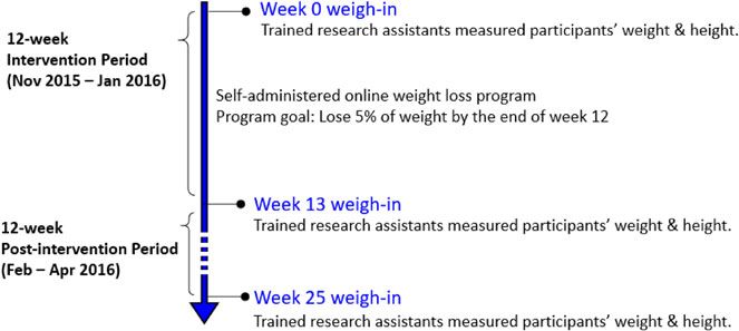
Behavioural Public Policy               3

           time-inconsistent preferences (Downs & Loewenstein, 2011). When people are
           present-biased, the immediate costs of undertaking a weight loss regime (increasing
           exercise, switching to a healthy diet) and the immediate enjoyment of eating
           unhealthy food are more salient, in comparison with the future benefits of weight
           loss (e.g., reduced risks of chronic diseases such as heart disease and Type 2 diabetes)
           and the future costs of being overweight (e.g., reduced quality of life and medical
           expenses). Consequently, there is a tendency to assign too little weight to future pay-
           offs relative to immediate payoffs in decision making; this tendency is often referred
           to as ‘hyperbolic discounting.’ (For evidence, see Loewenstein & Thaler, 1989; Ainslie
           1991, 1992; Akerlof, 1991; Loewenstein & Prelec, 1992; Ainslie & Haslam 1992a,
           1992b; Laibson, 1997; O’Donoghue & Rabin, 1999). Financial incentives serve to
           add an immediate reward for weight loss, thereby tipping the cost-benefit tradeoff
           toward behavioral change.
               The notion that financial incentives could motivate weight loss has been supported
           by a body of evidence acquired through proof-of-concept studies (i.e., ‘Wave 1’ stud-
           ies; List 2020) (Finkelstein et al., 2007, 2017; Volpp et al., 2008; John et al., 2011;
           Kullgren et al., 2013). These studies, like many other proof-of-concept studies,
           used relatively homogeneous participant samples and restricted experimental settings;
           therefore, the generalizability of their findings remains unclear. In terms of partici-
           pant samples, these RCTs have focused on either predominantly (i.e., >75%) male
           (Volpp et al., 2008; John et al., 2011) or female participants (Finkelstein et al.,
           2007; Kullgren et al., 2013). Moreover, the sample sizes of these studies were not
           large enough for a statistical evaluation of gender difference (sample sizes of these
           studies ranged from 57 to 207; all employed a three-arm design). In terms of experi-
           mental setting, many of these RCTs were conducted in clinical contexts (e.g., medical
           centers and hospitals in Volpp et al., 2008, John et al., 2011, Kullgren et al., 2013, and
           Finkelstein et al., 2017). These contexts were distinct from large-scale rollouts in
           which healthcare providers’ involvement is minimal.
               Our RCT was a ‘Wave 2’ study (List 2020) that built on the foundations of the pre-
           vious Wave 1 studies. Our primary goal was to evaluate the effects of weight loss incen-
           tives (IW) in a context that more resembled a community rollout. Our RCT met two
           important criteria that defined it as a Wave 2 study: First, it involved a heterogeneous
           group of participants recruited from all over Singapore through publicly accessible
           media (nationwide newspaper advertisements). Moreover, it had a sample size of 472,
           making it possible to examine gender difference in the effect of incentives on weight
           loss. Second, we examined the impact of IW in an experimental setting that is much
           more scalable, specifically, in the context of an online self-directed weight loss program.
               The literature has documented evidence from other Wave 2 studies conducted
           based on workplace wellness programs with larger sample sizes (e.g., Cawley &
           Price, 2013; Misra-Hebert et al., 2016). Notably, Cawley and Price (2013) found
           only modest effect of financial incentives on weight loss, which contrasts with the bet-
           ter outcomes reported in previous proof-of-concept studies and suggests a potential
           ‘voltage drop’ problem. Nevertheless, these findings must be interpreted with the cav-
           eat that randomized designs were not used in these studies. Other weight loss studies
           that did not employ a randomized design or did not use an intent-to-treat (ITT) ana-
           lysis are not discussed further (see Ananthapavan et al., 2018).

Downloaded from https://www.cambridge.org/core. IP address: 46.4.80.155, on 03 Jan 2022 at 03:13:40, subject to the Cambridge Core terms of
use, available at https://www.cambridge.org/core/terms. https://doi.org/10.1017/bpp.2021.20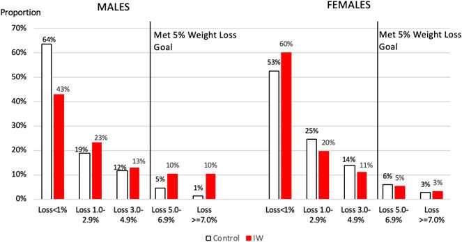
4       Catherine Yeung et al.

             Research design
             The online weight loss program
             A 12-week, self-administered online weight loss was a program based on the
             University of Pittsburg’s Lifestyle Balance Program (The DPP Research Group,
             2002). The following topics were covered in the program, in sequence: (1) The
             risks of being overweight; (2) Be a smart eater; (3) Healthy eating; (4) Move those
             muscles; (5) Tip the calorie balance; (6) Take charge of what’s around you; (7)
             Problem solving; (8) Healthy eating while out; (9) The slippery slope of lifestyle
             change; (10) Jump start your physical activity plan; (11) Eating and exercising
             while away; and (12) Preparing for self-management. The RCT was conducted in
             Singapore; therefore, the content was adapted for the local culture, diet, and lifestyle;
             it was also modified to suit bite-size e-learning. The material was developed by the
             research team and verified by a clinical team consisting of an endocrinologist, a
             psychologist, a physiotherapist, and two dieticians.
                The online program was delivered through 12 weekly sessions. All participants were
             enrolled in the same online program, had access to the videos, and were given a weight
             loss goal of 5% of their baseline body weight by the end of the program.

             RCT design and timeline
             There were two arms in this RCT: (1) Control arm with no financial incentive for
             weight loss and (2) IW arm with a US$150 (S$200) incentive for losing at least 5%
             of baseline weight by the end of the program. In other words, although all participants
             were given the goal of losing 5% of weight and had access to the online program, only
             those in the IW arm were incentivized to meet the 5% weight loss goal.2
                 The RCT consisted of two periods: a 12-week intervention and a 12-week post-
             intervention (Figure 1). Participant weight was measured by trained research assistants
             at three points: right before the intervention (at Week 0), at the end of the intervention
             (at Week 13), and at the end of the post-intervention period (Week 25). All participants
             received US$65 (S$88) as a participation fee for attending all three weigh-ins. This
             amount was split into two payments: US$15 was paid at the Week 13 weigh-in and
             US$50, at the Week 25 weigh-in. The IW incentive was tied to attendance at all
             three weigh-ins and was paid at the Week 25 weigh-in.

             Participants: selection criteria, recruitment, and randomization
             The weight loss program was a nationwide program conducted in Singapore.
             Participants had to meet the following eligibility criteria: age between 40 and 60;
             body mass index (BMI) between 23 and 33 kg/m2; not pregnant or planning to get

                2
                 As part of our overall research program on online weight loss management, we also included another
             arm that was unrelated to financial incentives for weight loss during the same time we conducted the IW
             and Control arms. This arm tested how incentivizing participants to acquire knowledge by watching videos
             on lifestyle changes in the online program may motivate weight loss. The preliminary results are available
             from the authors upon request.

Downloaded from https://www.cambridge.org/core. IP address: 46.4.80.155, on 03 Jan 2022 at 03:13:40, subject to the Cambridge Core terms of
use, available at https://www.cambridge.org/core/terms. https://doi.org/10.1017/bpp.2021.20
Behavioural Public Policy 5
Figure 1. Timeline of the RCT.
pregnant; free from chronic diseases that require medical attention, including dia-
betes, cardiovascular disease, high blood pressure, and lung disease. A BMI of
23 kg/m2 was chosen as Asian individuals above this BMI are considered to be over-
weight and at a greater risk for cardiometabolic complications (WHO Expert
Consultation, 2004). The BMI upper limit of 33 kg/m2 was chosen to minimize the
influence of outliers on the main result of weight loss, as less than 5% of the
Singapore population has a BMI of 34 kg/m2 and higher according to a National
Health Survey conducted by the Singapore Ministry of Health in 2004. The exclusion
criteria concerning chronic diseases were imposed to ensure that participants were
medically suited to undertake a self-administered weight loss program. All selection
criteria were set before subject recruitment commenced.
Participants were recruited from the public through newspaper advertisements.
The newspaper advertisement provided the general public with the following key
information: (1) the program was an online weight loss program with the objective
of helping participants lose 5% of their body weight; (2) the participants could
earn a participation fee of S$88 (US$65); and (3) participants must be 40–60 years
old with a BMI between 23 and 33. The recruitment advertisement is shown in
Appendix A. Potential participants were invited to visit a website for an initial screen-
ing. Those who passed the screening were invited to attend a weigh-in session at
Week 0, where they had their weight and height measured, age verified, and other
baseline measures collected. They were advised to log in to the program’s website
after the weigh-in.
Randomization took place when the participants first logged on to the website.
The randomization sequence followed a stratified block randomization scheme
with 8 gender-ethnicity strata [2 (Male, Female) × 4 (Chinese, Malay, Indian,
Others)3]. In other words, the participants were first sorted by gender and ethnicity,
3
The population of Singapore is categorized into four main groups: Chinese, Malays, Indians, and
Others. Since we anticipated citizens from all the four groups to take part in the weight loss program,
we stratified ethnicity to ensure balance in treatment assignment.
Downloaded from https://www.cambridge.org/core. IP address: 46.4.80.155, on 03 Jan 2022 at 03:13:40, subject to the Cambridge Core terms of
use, available at https://www.cambridge.org/core/terms. https://doi.org/10.1017/bpp.2021.206 Catherine Yeung et al.
and then randomly assigned to one of two arms. After randomization, information
on the additional financial incentives offered in the IW arm was shown to partici-
pants via an automated message shown onscreen. A total of 472 participants (of
which 171 were males) were randomly assigned to one of the two arms4.
Outcome measures
The first outcome of interest was weight loss after 12 weeks (measured at Week 13),
which revealed whether IW led to a greater weight loss. To provide an unbiased
comparison of weight loss between genders, we chose percentage weight loss rather
than absolute weight loss as the unit of analysis because the former accounted for
baseline weight differences between the two genders. Percentage weight loss was
defined as the difference in weight between Week 13 and Week 0, divided by weight
at Week 0.
Weight loss outcomes were analyzed using both the ITT approach and the per-
protocol (PP) approach as a strategy to handle the potential effects of non-
compliance on our empirical tests. In the ITT analysis, participants who did not
attend a weigh-in were still included in the analysis and were treated as having the
same weight at Week 0. The PP approach included only the participants
who attended all three weigh-ins. The ITT approach relies solely on an exogenous
source of variation (i.e., randomization procedure) and is free from other endogenous
sources of influence (e.g., selection bias introduced by dropout); therefore,
it provides the cleanest possible evaluation of treatment effects from a methodological
standpoint (for further discussion of why the ITT approach is the standard
approach in the analysis of any RCT, see Glennerster & Takavarasha, 2013).
Nevertheless, the PP approach informs us the effect of a treatment conditional on
compliance to experimental requirements. Hence, the two approaches together
constitute a sensitivity analysis to verify that our results hold, irrespective of (non-)
compliance issues. Throughout our article, we discuss our results based on the
ITT approach, but we present the PP analysis results alongside the ITT results in
tables.
To control the family-wise error rate, we performed multiple hypothesis testing
(MHT) and reported MHT-adjusted p-values for statistically significant results.
MHT was conducted based on the resampling-based stepdown method developed
by Romano and Wolf (2005a, 2005b, 2016) with 1000 bootstrap replications.5 We
also collected data on weekly exercise level and diet quality; such responses were self-
reported on a voluntary basis. Readers who are interested in these measurements can
refer to Appendix B.
4
With the sample size of 472 with equal probability of control and treatment, we can detect the standard
effect size of 0.26 with power 0.8 and significance level of 0.05. For males, with the sample size of 170 with
the equal probability of control and treatment, we can detect the standard effect size of 0.43 with power 0.8
and significance level of 0.05. For females, with the sample size of 300 with the equal probability of control
and treatment, we can detect the standard effect size of 0.33 with power 0.8 and significance level of 0.05.
5
We have also conducted multiple hypothesis testing using the method from List et al. (2019); the results
do not change.
Downloaded from https://www.cambridge.org/core. IP address: 46.4.80.155, on 03 Jan 2022 at 03:13:40, subject to the Cambridge Core terms of
use, available at https://www.cambridge.org/core/terms. https://doi.org/10.1017/bpp.2021.20Behavioural Public Policy 7
Estimation strategy
To evaluate the effect of the incentive on the weight loss and its differential effect by
gender, we estimate the following ordinary least squares (OLS) regression:
yi = a + b1 IWi + b2 Malei + b3 IW∗Malei + X ′i m + 1i (1)
where yi is the main outcome: the percentage of weight loss at Week 13 or at Week 25,
IWi, is the dummy variable for the treatment group, Malei is the indicator for male
participants, and IW*Malei is the interaction term between the treatment status and
the gender dummy. Xi includes the covariates: the baseline BMI, age, and educational
level. Throughout we run OLS regressions with heteroscedasticity-consistent standard
errors.
Results
Participant characteristics and attrition
A total of 472 participants were randomly assigned to one of the two arms (males:
Control = 85, IW = 86; females: Control = 150, IW = 151). Of the 472 participants
we recruited, 171 were male. Our male participants were 47.8 years old on average
(SD = 4.8), with an average BMI of 27.0 kg/m2 (SD = 2.5). Our female participants
were 48.9 years old on average (SD = 5.4), with an average BMI of 26.6 kg/m2 (SD =
2.5). Other participant characteristics are shown in Table 1. Statistical tests were
conducted separately for each baseline measure. In terms of age, BMI, and educa-
tion levels, males had a slightly higher BMI than females (F(1, 468) = 3.54, p = 0.06),
were on average one year younger than females (F(1, 468) = 4.63, p = 0.03), and
had higher levels of education (Mantel–Haenszel test: χ 2(1) = 16.40, p < 0.001).
Males also had higher levels of income than females (Mantel–Haenszel test:
χ 2(1) = 33.73, p < 0.001; this result remains the same if the ‘no income’ category
was excluded: χ 2(1) = 31.36, p < 0.001).
Within each gender, there were no differences in age, baseline BMI, income levels,
and educational levels between the two arms. We also asked the participants to pre-
dict their weight in 3 months. There were no differences in expected weight loss
across arms for each gender. There were no other differences in baseline measures.
To ensure the robustness of our findings, we report models with and without baseline
BMI, age, and educational level as controls.
Attrition is defined as no-shows for the Week 13 or Week 25 weigh-in. Among the
males, the Week 13 attrition rates for the Control and IW conditions were 22.35%
and 8.14%, respectively (χ 2 = 6.89, df = 1, p = .01). Among the females, the Week 13
attrition rates for these conditions were 18.67% and 17.22%, respectively (χ 2 = 0.11,
df = 1, p = 0.74). At Week 25, the overall attrition rate was 15.7%; there were no dif-
ferences across the two conditions for males (Control: 16.47%, IW: 10.47%; χ 2 = 1.32,
df = 1, p = 0.25) and females (Control: 17.33%, IW: 16.56%; χ 2 = 0.03, df = 1,
p = 0.86). To handle attrition, we report results using the ITT approach by assuming
that the participants who did not show up at the weigh-ins remained at their baseline
weights.
Downloaded from https://www.cambridge.org/core. IP address: 46.4.80.155, on 03 Jan 2022 at 03:13:40, subject to the Cambridge Core terms of
use, available at https://www.cambridge.org/core/terms. https://doi.org/10.1017/bpp.2021.208 Catherine Yeung et al.
Table 1. Baseline measures by gender and treatment arm.
Males Females
Control IW Overall Control IW Overall
(n = 85) (n = 86) (n = 171) (n = 150) (n = 151) (n = 301)
Age, Mean (SD) 48.3 (4.9) 47.3 (4.7) 47.8 (4.8) 49.2 (5.5) 48.6 (5.3) 48.9 (5.4)
BMI, Mean (SD) 27.1 (2.7) 27.0 (2.3) 27.0 (2.5) 26.7 (2.6) 26.5 (2.4) 26.6 (2.5)
Weight in kg, mean (SD) 79.9 (9.3) 78.1 (9.9) 79.0 (9.6) 66.4 (7.9) 66.7 (8.1) 66.5 (8.0)
Education
Lower secondary 0.0% 4.7% 2.3% 0.7% 1.3% 1.0%
Secondary 11.8% 10.5% 11.1% 21.3% 22.5% 21.9%
Post-secondary 27.1% 20.9% 24.0% 39.3% 35.8% 37.5%
University 61.2% 64.0% 62.6% 38.7% 40.4% 39.5%
Income (in SGD)
No income 11.8% 3.5% 7.6% 12.7% 15.2% 14.0%
Below 3000 16.5% 10.5% 13.5% 34.0% 31.1% 32.6%
3000–4999 29.4% 34.9% 32.2% 27.3% 30.5% 28.9%
5000–6999 10.6% 22.1% 16.4% 13.3% 9.3% 11.3%
7000 and above 31.8% 29.1% 30.4% 12.7% 13.9% 13.3%
Race
Chinese 83.5% 83.7% 83.6% 88.0% 87.4% 87.7%
1
Asian 14.1% 11.6% 12.9% 10.7% 11.3% 11.0%
Other 2.4% 4.7% 3.5% 1.3% 1.3% 1.3%
Expected weight 4.5% (2.9) 4.9% (2.9) 4.7% (2.9) 5.1% (3.6) 4.7% (3.3) 4.9% (3.4)
loss, mean (SD)2
Notes:
1
Includes Indian, Malay, Indonesian, Filipino, Thai, Arab, Sri Lankan, and Burmese.
2
Participants were asked to predict their weight (in kg) in 3 months, upon program completion. Expected weight loss in
% of initial weight was computed as weight loss divided by baseline weight.
Weight loss at Week 13
We first evaluated the effects of incentive on male and female weight loss at Week 13.
In Table 2, we show the OLS regression results: columns (1) and (2) show those using
the ITT approach, and columns (3) and (4), the PP sample. An OLS regression
(model (1), Table 2) yielded a nonsignificant main effect of gender (p = 0.11) and
a significant incentive × gender interaction (p < 0.001; MHT-adjusted p = 0.002).
In Figure 2, the left panel shows the average percentage weight loss at Week 13. For
males, the average weight loss percentage was higher in the IW (2.40%) than in the
Control (0.87%) (F(1, 468) = 11.79, p < 0.001; MHT-adjusted p = 0.006), indicating
that the financial incentive promoted greater weight loss among males. For females,
we did not detect any difference in weight loss between the IW arm (1.03%) and the
Downloaded from https://www.cambridge.org/core. IP address: 46.4.80.155, on 03 Jan 2022 at 03:13:40, subject to the Cambridge Core terms of
use, available at https://www.cambridge.org/core/terms. https://doi.org/10.1017/bpp.2021.20Behavioural Public Policy 9
Table 2. Regression results of treatment and gender effects on percentage weight loss at Week 13.
Percentage weight loss at Week 13
ITT Per-Protocol
Sample (1) (2) (3) (4)
Gender = Male −0.571 −0.619* −0.712 −0.702
(0.112) (0.076) (0.112) (0.111)
[0.200] [0.142] [0.119] [0.192]
IW −0.409 −0.381 −0.571 −0.530
(0.163) (0.178) (0.103) (0.120)
[0.347] [0.391] [0.238] [0.272]
Gender = Male * IW 1.938*** 1.942*** 2.016*** 2.041***
(0.000) (0.000) (0.001) (0.001)
[0.002] [0.002] [0.003] [0.005]
Baseline BMI −0.084* −0.089
(0.088) (0.135)
Age 0.056** 0.055*
(0.046) (0.096)
Education = Secondary −0.551 −0.058
(0.449) (0.950)
Education = Post-Secondary 0.200 0.775
(0.779) (0.397)
Education = University 0.481 0.942
(0.495) (0.292)
N 472 472 385 385
2
r 0.037 0.068 0.032 0.058
Control means of dependent 1.443 1.443 1.834 1.834
variable
t-test (p-value)
IW + (Male * IW) = 0 0.001 0.001 0.006 0.004
Male + (Male * IW) = 0 0.001 0.001 0.004 0.004
Note. This table presents the OLS regression coefficient estimates, with p-values in parentheses. MHT-adjusted p-values
are shown in [brackets]. Dependent variables are Week 13 weight loss [−(Week 13 weight − Week 0 weight)/Week 0
weight] * 100. Control and Female are used as the reference categories. Regression models (1) and (2) are constructed
using the ITT approach, whereas models (3) and (4), the PP approach.
*, **, ***indicate statistical significance at the 5%, 1%, and 0.5% levels, respectively.
Control arm (1.44%) (p = 0.16). Next, we compared weight loss across gender. In the
IW arm, the weight loss percentage was higher for males than for females (2.40% for
males vs. 1.03% for females) (F(1, 468) = 12.01, p < 0.001; MHT-adjusted p = 0.002).
In the Control arm, there was no difference in weight loss between genders (0.87% for
males and 1.44% for females; p = 0.11).
Downloaded from https://www.cambridge.org/core. IP address: 46.4.80.155, on 03 Jan 2022 at 03:13:40, subject to the Cambridge Core terms of
use, available at https://www.cambridge.org/core/terms. https://doi.org/10.1017/bpp.2021.2010 Catherine Yeung et al.
Figure 2. Weight loss at Week 13. Error bars show 95% CI. n = 472.
For robustness, we ran regression models with and without control variables. The
odd-numbered columns of Table 2 show the regression results without the control
variables, whereas the even-numbered columns show those with the controls (base-
line BMI, age, and educational level). Qualitatively, the addition of the control vari-
ables has little impact on treatment effect point estimates. Importantly, these results
show that the gender difference is robust using both the ITT and PP approaches, and
independent of participants’ BMI, age, and education level.
Weight loss target met at Week 13
In Figure 2, the right panel displays the proportion of participants in each arm who
met the 5% weight loss target. We fitted a binary logistic regression on success in
meeting the target and conducted pairwise comparisons based on the model. We
found that 20.93% of males in the IW arm achieved the weight loss target, higher
than the 5.88% in the Control; the difference was statistically significant (IW vs.
Control: χ 2(1) = 8.72, p < 0.01; MHT-adjusted p = 0.01). For females, there were no
differences across the two arms, with 8.67% and 8.61% of participants meeting the
target in the Control and IW arms, respectively.
We next examined whether the greater weight loss among males in the IW arm
was driven only by those who met the weight loss target. See Figure 3, which
shows the proportion of participants by various weight loss outcomes in each arm.
The proportion of males who recorded weight loss of 1% or less (this includes
some participants who had gained weight) was lower in the IW arm (43.0%) than
the Control (63.5%) (diff = 20.5%, χ 2(1) = 7.45, p < 0.01). Moreover, an OLS regres-
sion conducted based on the subsample of participants who did not meet the 5% tar-
get (148 males, 275 females) using Week 13 weight loss as the dependent variable
showed that the incentive × gender interaction was still significant (p < 0.01;
MHT-adjusted p = 0.01), and percentage weight loss was still higher among
males in the IW (1.09%) than males in the Control (0.44%) arm, F(1, 419) = 4.45,
Downloaded from https://www.cambridge.org/core. IP address: 46.4.80.155, on 03 Jan 2022 at 03:13:40, subject to the Cambridge Core terms of
use, available at https://www.cambridge.org/core/terms. https://doi.org/10.1017/bpp.2021.20Behavioural Public Policy 11
Figure 3. Proportion of participants by weight loss outcomes, Week 13.
p = 0.04; MHT-adjusted p = 0.07). Hence, the greater weight loss in the IW arm
achieved by males was driven not only by participants who met the weight loss target,
but also those who did not; in contrast, no such effect of IW was observed in females.
Weight loss at Week 25 (post-intervention)
Figure 4 shows weight loss at Week 25. Table 3 displays the OLS regression results.
Similar to the results for Week 13 weight loss, the OLS regression (model (1),
Table 3) shows a nonsignificant main effect of gender (p = 0.13), with a significant
incentive type × gender interaction (p = 0.02; MHT-adjusted p = 0.03). Among
males, weight loss in the IW arm (2.53%) remained higher than in the Control
arm (0.88%) (F(1, 468) = 9.68; p < 0.005; MHT-adjusted p = 0.01). In other words,
Figure 4. Weight loss at Week 25 by
treatment and gender. Error bars
show 95% CI. n = 472.
Downloaded from https://www.cambridge.org/core. IP address: 46.4.80.155, on 03 Jan 2022 at 03:13:40, subject to the Cambridge Core terms of
use, available at https://www.cambridge.org/core/terms. https://doi.org/10.1017/bpp.2021.2012 Catherine Yeung et al.
Table 3. Regression results of treatment and gender effects on percentage weight loss at Week 25.
Percentage weight loss at Week 25
ITT Per-protocol
Sample (1) (2) (3) (4)
Gender = Male −0.669 −0.656 −1.000* −0.901*
(0.131) (0.127) (0.061) (0.083)
[0.200] [0.186] [0.111] [0.192]
IW 0.107 0.177 −0.139 −0.055
(0.786) (0.644) (0.759) (0.900)
[0.952] [0.853] [0.930] [0.983]
Gender = Male * IW 1.537** 1.601** 1.821** 1.879**
(0.020) (0.016) (0.018) (0.015)
[0.030] [0.028] [0.033] [0.036]
Baseline BMI −0.091 −0.065
(0.149) (0.392)
Age 0.101*** 0.089**
(0.005) (0.027)
Education = Secondary 0.457 0.359
(0.490) (0.706)
Education = Post-Secondary 1.410** 1.362
(0.032) (0.149)
Education = University 1.494** 1.180
(0.018) (0.190)
N 472 472 385 385
2
r 0.021 0.056 0.020 0.044
Control means of dependent variable 1.552 1.552 2.141 2.141
t-test (p-value)
IW + (Male * IW) = 0 0.002 0.001 0.007 0.004
Male + (Male * IW) = 0 0.077 0.061 0.138 0.088
Note. This table presents the OLS regression coefficient estimates, with p-values in parentheses. MHT-adjusted p-values
are shown in [brackets]. Dependent variables are Week 25 weight loss [−(Week 25 weight − Week 0 weight)/Week 0
weight] * 100. Control and Female are used as the reference categories. Regression models (1) and (2) are constructed
using the ITT approach; models (3) and (4) are constructed using the per-protocol approach.
*, **, *** indicate statistical significance at the 5%, 1%, and 0.5% levels, respectively.
for males, the effect of IW sustained for at least 3 months after the incentive was
removed. For females, as in Week 13, there remained no differences in weight loss
at Week 25 between the IW (1.66%) and Control (1.55%) arms (p = 0.79).
Next, we compared weight loss across gender. In the IW arm, the weight loss per-
centage was higher for males (2.53%) than for females (1.66%), but the difference was
only marginally significant (p = 0.08). In the Control arm, the weight loss percentage
in males (0.88%) was not different than that in females (1.55%) (p = 0.23).
Downloaded from https://www.cambridge.org/core. IP address: 46.4.80.155, on 03 Jan 2022 at 03:13:40, subject to the Cambridge Core terms of
use, available at https://www.cambridge.org/core/terms. https://doi.org/10.1017/bpp.2021.20Behavioural Public Policy 13
General discussion
This article shows that offering overweight males and females a significant financial
incentive to meet a weight loss target (IW) works only for males. Our findings refute
the commonly held assumption that financial incentives for weight loss work equally
well for the two genders. To the best of our knowledge, none of the weight loss incen-
tives currently in use assume a gender difference in response to such incentives. This
is perhaps unsurprising since research so far has not provided any evidence of such a
gender difference (see our literature review). Notably, however, the lack of evidence is
due to the lack of testing, rather than observing supportive evidence of no difference.
Our findings fill this gap by showing strong evidence of gender difference and provide
implications for both theoretical research and behaviorally informed weight loss policies.
SANS conditions and generalizability of findings
To help policy makers assess the generalizability of our findings, we follow List
(2020)’s recommendation and report the four transparency conditions (SANS condi-
tions) – selection, attrition, naturalness, and scaling.
Selection
We compared our sample to the national population between the age of 40 and 60 in
terms of educational level, income, and race (see Appendix C). Our participants were
largely comparable to the population in these aspects, which suggests that our recruit-
ment reached a considerably heterogeneous group of people from the general public.
Since we did not have a ‘nonparticipant’ group for comparison in our RCT, we are
unable to evaluate the extent of volunteering bias. In general, we expect people who vol-
unteer to participate in a weight loss program to be more motivated to lose weight than
those who do not volunteer to join. Hence, we expect our findings to be generalizable to
community-level weight loss programs, where participation is usually voluntary.
Attrition
We present an attrition analysis in the section ‘Participant characteristics and attri-
tion’ and participant flow in Figure 5. There could be several reasons for participant
no-shows. First, some participants were simply too busy or forgot to attend. Second,
participants who had not qualified for the IW reward (i.e., either not in the IW arm
or failed to meet the weight loss target) had a lower incentive to attend the weigh-ins
than those who did (i.e., those in the IW arm and met the 5% weight loss target).
Third, participants who were disengaged from the program might be less motivated
to attend the weigh-ins than those who had been actively engaged, despite not having
met the weight loss target. The second and third reasons could potentially introduce
selection bias to our RCT. The standard approach to handle attrition in weight loss
study is to report results using the ITT approach by assuming that the participants
who did not show up at the weigh-ins remained at their baseline weights (see, e.g.,
Volpp et al., 2008). We used the same approach in our data analysis. A supplemen-
tary analysis was also conducted using the PP approach, which included only the par-
ticipants who attended all three weigh-ins.
Downloaded from https://www.cambridge.org/core. IP address: 46.4.80.155, on 03 Jan 2022 at 03:13:40, subject to the Cambridge Core terms of
use, available at https://www.cambridge.org/core/terms. https://doi.org/10.1017/bpp.2021.2014 Catherine Yeung et al.
Figure 5. Diagram of participant flow.
Naturalness
The RCT was a real-world intervention conducted in a highly natural setting. The
weight loss program was fully adapted to the context of self-directed weight loss.
The weight loss program was hosted online with no mandatory requirements for
participants to follow any of the health recommendations. Along the same lines,
we refrained from arranging any online meetings with healthcare providers for the
participants, nor did we give the participants personalized dietary feedback, even
though such features may be effective in promoting weight loss (Tate et al., 2001;
Gold et al., 2007). Therefore, our setting highly resembles large-scale rollouts of self-
directed weight loss programs.
Scaling
Our findings show that the ‘voltage drop’ problem could happen for large-scale weight
loss programs that employ financial incentives to motivate weight loss – if financial
incentives for weight loss work only for one gender, we would expect a significant
voltage drop when incentives for weight loss are offered to the general population.
Potential explanations for the gender difference in financial incentives for
weight loss
Why were our male participants more driven by IW to lose weight? Our RCT did not
allow us to identify the mechanism behind the gender difference observed; neverthe-
less, we discuss some possible explanations for our findings.
One possibility would be that the male participants were more driven by IW
because they had less income than the female participants. However, this was unlikely
to be the case because in our study, the male participants earned higher income than
the female participants.
Downloaded from https://www.cambridge.org/core. IP address: 46.4.80.155, on 03 Jan 2022 at 03:13:40, subject to the Cambridge Core terms of
use, available at https://www.cambridge.org/core/terms. https://doi.org/10.1017/bpp.2021.20Behavioural Public Policy 15
Another possibility would be that the female participants were less responsive to
financial incentives for weight loss, because there is a stronger pairing between weight
management and social rewards in females. Indeed, there is an extensive literature
that documents differences between men and women in the type of rewards they
seek from weight management.
In many societies, there is a stronger emphasis on women’s physical appearance
than on men’s. Women are more vulnerable to weight discrimination than men:
While men do not experience notable weight discrimination until their BMI reaches
35, women feel discriminated at the much lower BMI level of 27 (Puhl et al., 2008).
Judgment of physical appearance comes along with implications to romantic relation-
ships, popularity, and employment, making the social implications of physical
appearance a lot more significant for women than men (Feingold, 1990, 1992).
Finally, in a weight loss program, women were more likely than men to report
improving personal esteem (e.g., improve appearance, feel better about oneself) as
a motivator than men (Crane et al., 2017). Overall, these streams of research suggest
that social rewards may have a stronger motivational significance for women than
men in the domain of weight management, so that the financial incentives for weight
loss may be relatively less attractive to the former. In this regard, women may benefit
more from programs that motivate weight loss through social incentives (e.g.,
face-to-face guided programs, group weight loss programs).
Implications for behaviorally informed policies
Recently, behavioral scientists and economists have raised their attention to the role of
demographics for their critical relevance to the success of scaled implementation of
behavioral interventions. Specifically, the assumption that an intervention would
work equally well for all demographic groups is a major cause of ‘voltage drop’ –
the phenomenon that the effect size of an intervention drops significantly relative
to that reported in the original research when it is implemented at a large scale in
the society (Banerjee et al., 2018; Al-Ubaydli et al., 2019a, 2019b; Ho et al., 2021).
The same could occur for large-scale weight loss programs that use financial incen-
tives to motivate weight loss, because financial incentives for weight loss work only
for one gender. Future research could experiment combining financial incentives
with other gender-specific behavioral interventions (e.g., online discussion forum,
which works well to promote women weight loss; Johnson & Wardle, 2011) to pro-
duce more promising and gender-balanced overall results. In this respect, behavioral
scientists who run commercial weight loss programs would be in a favorable position
to analyze their data to examine gender difference in their incentive programs, and
customize weight loss options to achieve greater effectiveness. Notably, our findings
do not suggest a policy that offers money for men to lose weight but not to
women; rather, they suggest that policy makers may consider offering different incen-
tive options and letting the respondents pick the one that will best motivate them.
Potential limitations
We conclude with three limitations. First, we provided a cash incentive of $150 for
achieving 5% weight loss. People’s responses to the $150 weight loss incentive depend
Downloaded from https://www.cambridge.org/core. IP address: 46.4.80.155, on 03 Jan 2022 at 03:13:40, subject to the Cambridge Core terms of
use, available at https://www.cambridge.org/core/terms. https://doi.org/10.1017/bpp.2021.2016 Catherine Yeung et al.
on how much they value the benefit of an incremental $150 cash reward, in addition
to the benefit of losing weight. For example, severely overweight people may not
require the extra $150 for them to weight loss, so we may observe no effect if the
$150 were offered to them. For a similar reason, it is also unclear if one would obtain
the same pattern of results with an incentive of a substantially different monetary
value. Second, we had only one post-intervention weigh-in (12 weeks after the end
of the program) and are thus unable to conclude if the greater weight loss among
males in the IW arm persisted beyond the 24-week timeframe. Also, we did not
draw blood for analysis, so we were unable to evaluate any health benefits beyond
weight loss (e.g., reducing cardiometabolic risk). Third, since RCT relied on partici-
pants’ voluntary signup, there was a potential for volunteer bias in our recruitment.
Nevertheless, considering that most community-level weight loss programs are orga-
nized on a volunteer basis, we would expect our findings to be generalizable to such
contexts.
Funding. This work was supported by the Global Asia Institute, National University of Singapore
(NIHA-2013-1-001) and the Singapore National Research Foundation’s Returning Singaporean Scientists
Scheme (grant no. NRFRSS2014-001). The funding sources had no involvement in the conduct of the
research or preparation of the manuscript.
Conflict of interest. None.
References
Ainslie, G. (1991), ‘Derivation of rational economic behavior from hyperbolic discount curves’, American
Economic Review, 81(2): 334–340.
Ainslie, G. (1992), Picoeconomics: The strategic interaction of successive motivational states within the per-
son. New York: Cambridge University Press.
Ainslie, G. and N. Haslam (1992a), ‘Self- control’, in G. Loewenstein and J. Elster (eds), Choice over time,
New York: Russell Sage Foundation.
Ainslie, G. and N. Haslam (1992b), ‘Hyperbolic discounting’, in G. Loewenstein and J. Elster (eds), Choice
over time, New York: Russell Sage Foundation.
Akerlof, G. A. (1991), ‘Procrastination and obedience’, The American Economic Review, 81(2): 1–19.
Al-Ubaydli, O., M. S. Lee, J. A. List, C. Mackevicius and D. Suskind (2019a), How can experiments play a
greater role in public policy? 12 proposals from an economic model of scaling. University of Chicago,
Becker Friedman Institute for Economics Working Paper (2019-131). doi:10.2139/ssrn.3478066.
Al-Ubaydli, O., J. A. List and D. Suskind (2019b), The science of using science: Towards an understanding of
the threats to scaling experiments. University of Chicago, Becker Friedman Institute for Economics
Working Paper (2019–73). doi:10.2139/ssrn.3391481.
Ananthapavan, J., A. Peterson and G. Sacks (2018), ‘Paying people to lose weight: The effectiveness of
financial incentives provided by health insurers for the prevention and management of overweight
and obesity—A systematic review’, Obesity Reviews, 19(5): 605–613. doi:10.1111/obr.12657.
Banerjee, A., S. Barnhardt and E. Duflo (2018), ‘Can iron-fortified salt control anemia? Evidence from two
experiments in rural Bihar’, Journal of Development Economics, 133(July): 127–146. doi:10.1016/
j.jdeveco.2017.12.004.
Cawley, J. and J. A. Price (2013), ‘A case study of a workplace wellness program that offers financial incen-
tives for weight loss’, Journal of Health Economics, 32(5): 794–803. doi:10.1016/j.jhealeco.2013.04.005.
Crane, M. M., R. W. Jeffery and N. E. Sherwood (2017), ‘Exploring gender differences in a randomized trial
of weight loss maintenance’, American Journal of Men’s Health, 11(2): 369–375. doi:10.1177/
1557988316681221.
Downs, J. S. and G. Loewenstein (2011), ‘Behavioral economics and obesity’, in J. Cawley (ed.), The Oxford
handbook of the social science of obesity, Chap. 9, New York: Oxford University Press.
Downloaded from https://www.cambridge.org/core. IP address: 46.4.80.155, on 03 Jan 2022 at 03:13:40, subject to the Cambridge Core terms of
use, available at https://www.cambridge.org/core/terms. https://doi.org/10.1017/bpp.2021.20Behavioural Public Policy 17
Fallah-Fini, S., A. Adam, L. J. Cheskin, S. M. Bartsch and B. Y. Lee (2017), ‘The additional costs and health
effects of a patient having overweight or obesity: A computational model’, Obesity, 25(10): 1809–1815.
doi:10.1002/oby.21965.
Feingold, A. (1990), ‘Gender differences in effects of physical attractiveness on romantic attraction: A com-
parison across five research paradigms’, Journal of Personality and Social Psychology, 59(5): 981–993.
doi:10.1037/0022-3514.59.5.981.
Feingold, A. (1992), ‘Gender differences in mate selection preferences: A test of the parental investment
model’, Psychological Bulletin, 112(1): 125–139. doi:10.1037/0033-2909.112.1.125.
Finkelstein, E. A., L. A. Linnan, D. F. Tate and B. E. Birken (2007), ‘A pilot study testing the effect of dif-
ferent levels of financial incentives on weight loss among overweight employees’, Journal of Occupational
and Environmental Medicine, 49(9): 981–989. doi:10.1097/JOM.0b013e31813c6dcb.
Finkelstein, E. A., K. W. Tham, B. A. Haaland and A. Sahasranaman (2017), ‘Applying economic incentives
to increase effectiveness of an outpatient weight loss program (TRIO) − A randomized controlled trial’,
Social Science & Medicine, 185(July): 63–70. doi:10.1016/j.socscimed.2017.05.030.
Fung, T. T., S. E. Chiuve, M. L. McCullough, K. M. Rexrode, G. Logroscino and F. B. Hu (2008), ‘Adherence
to a DASH-style diet and risk of coronary heart disease and stroke in women’, Archives of Internal
Medicine, 168(7): 713–720. doi:10.1001/archinte.168.7.713.
Glennerster, R. and K. Takavarasha (2013), Running randomized evaluations: A practical guide. Princeton,
NJ: Princeton University Press.
Gold, B. C., S. Burke, S. Pintauro, P. Buzzell and J. Harvey-Berino (2007), ‘Weight loss on the web: A pilot
study comparing a structured behavioral intervention to a commercial program’, Obesity, 15(1): 155–164.
Hayes, A. F. and K. J. Preacher (2014), ‘Statistical mediation analysis with a multicategorical independent
variable’, British Journal of Mathematical and Statistical Psychology, 67(3): 451–470. doi:10.1111/
bmsp.12028.
Ho, T. H., C. Leong and C. Yeung (2021), ‘Success at scale: six suggestions from implementation and policy
sciences’, Behavioural Public Policy, 5(1): 71–79. doi:10.1017/bpp.2020.20.
John, L. K., G. Loewenstein, A. B. Troxel, L. Norton, J. E. Fassbender and K. G. Volpp (2011), ‘Financial
incentives for extended weight loss: A randomized, controlled trial’, Journal of General Internal
Medicine, 26(6): 621–626. doi:10.1007/s11606-010-1628-y.
Johnson, F. and J. Wardle (2011), ‘The association between weight loss and engagement with a web-based
food and exercise diary in a commercial weight loss programme: A retrospective analysis’, International
Journal of Behavioral Nutrition and Physical Activity, 8(83): 1–7. doi:10.1186/1479-5868-8-83.
Kelly, T., W. Yang, C. S. Chen, K. Reynolds and J. He (2008), ‘Global burden of obesity in 2005 and projec-
tions to 2030’, International Journal of Obesity, 32(9): 1431–1437. doi:10.1038/ijo.2008.102.
Kullgren, J. T., A. B. Troxel, G. Loewenstein, D. A. Asch, L. A. Norton, L. Wesby, Y. Tao, J. Zhu and K.
G. Volpp (2013), ‘Individual-versus group-based financial incentives for weight loss: A randomized, con-
trolled trial’, Annals of Internal Medicine, 158(7): 505–514. doi:10.7326/0003-4819-158-7-201304020-
00002.
Laibson, D. (1997), ‘Golden eggs and hyperbolic discounting’, The Quarterly Journal of Economics, 112(2):
443–478.
List, J. A. (2020), Non Est Disputandum De Generalizability? A glimpse into the external validity trial. NBER
Working Paper No. w27535. Available at SSRN: https://ssrn.com/abstract=3658829.
List, J. A., M. S. Azeem and X. Yang (2019), ‘Multiple hypothesis testing in experimental economics’,
Experimental Economics, 22(4): 773–793.
Loewenstein, G. and D. Prelec (1992), ‘Anomalies in intertemporal choice: Evidence and an interpretation’,
The Quarterly Journal of Economics, 107(2): 573–597.
Loewenstein, G. and R. Thaler (1989), ‘Anomalies: Intertemporal choice’, Journal of Economic Perspectives,
3(4): 181–193.
Misra-Hebert, A. D., B. Hu, G. Taksler, R. Zimmerman and M. B. Rothberg (2016), ‘Financial incentives
and diabetes disease control in employees: A retrospective cohort analysis’, Journal of General Internal
Medicine, 31(8): 871–877. doi:10.1007/s11606-016-3686-2.
Ng, M., T. Fleming, M. Robinson, B. Thomson, N. Graetz, C. Margono and E. Gakidou (2014), ‘Global,
regional, and national prevalence of overweight and obesity in children and adults during 1980–2013:
A systematic analysis for the Global Burden of Disease Study 2013’, Lancet, 384(9945): 766–781.
O’Donoghue, T. and M. Rabin (1999), ‘Doing it now or later’, American Economic Review, 89(1): 103–124.
Downloaded from https://www.cambridge.org/core. IP address: 46.4.80.155, on 03 Jan 2022 at 03:13:40, subject to the Cambridge Core terms of
use, available at https://www.cambridge.org/core/terms. https://doi.org/10.1017/bpp.2021.2018 Catherine Yeung et al.
Puhl, R. M., T. Andreyeva and K. D. Brownell (2008), ‘Perceptions of weight discrimination: Prevalence and
comparison to race and gender discrimination in America’, International Journal of Obesity, 32(6): 992–
1000. doi:10.1038/ijo.2008.22.
Romano, J. P. and M. Wolf (2005a), ‘Exact and approximate stepdown methods for multiple hypothesis
testing’, Journal of the American Statistical Association, 100(469): 94–108.
Romano, J. and M. Wolf (2005b), ‘Stepwise multiple testing as formalized data snooping’, Econometrica,
73(4): 1237–1282.
Romano, J. and M. Wolf (2016), ‘Efficient computation of adjusted p-values for resampling-based stepdown
multiple testing’, Statistics and Probability Letters, 113(June): 38–40.
Stevens, G. A., G. M. Singh, Y. Lu, G. Danaei, J. K. Lin, M. M. Finucane, A. N. Bahalim, R. K. McIntire, H.
R. Gutierrez, M. Cowan, C. J. Paciorek, F. Farzadfar, L. Riley and M. Ezzati (2012), ‘National, regional,
and global trends in adult overweight and obesity prevalences’, Population Health Metrics, 10(1): 22.
doi:10.1186/1478-7954-10-22.
Tate, D. F., R. R. Wing and R. A. Winett (2001), ‘Using Internet technology to deliver a behavioral weight
loss program’, Journal of the American Medical Association, 285(9): 1172–1177.
The Diabetes Prevention Program (DPP) Research Group (2002), ‘The Diabetes Prevention Program
(DPP): Description of lifestyle intervention’, Diabetes Care, 25(12): 2165–2171. doi:10.2337/
diacare.25.12.2165.
Volpp, K. G., L. K. John, A. B. Troxel, L. Norton, J. Fassbender and G. Loewenstein (2008), ‘Financial
incentive-based approaches for weight loss: A randomized trial’, Journal of the American Medical
Association, 300(22): 2631–2637. doi:10.1001/jama.2008.804.
WHO Expert Consultation (2004), ‘Appropriate body-mass index for Asian populations and its implica-
tions for policy and intervention strategies’, Lancet (London, England), 363(9403): 157–163.
doi:10.1016/s0140-6736(03)15268-3.
Appendix A. Recruitment advertisement
Downloaded from https://www.cambridge.org/core. IP address: 46.4.80.155, on 03 Jan 2022 at 03:13:40, subject to the Cambridge Core terms of
use, available at https://www.cambridge.org/core/terms. https://doi.org/10.1017/bpp.2021.20Behavioural Public Policy 19
Appendix B. Diet and exercise: measurements and results
Self-reporting of diet and exercise
Each week, the website prompted participants to report the number of minutes they exercised over the pre-
vious week. These self-reports were voluntary; a total of 203 participants reported their exercise for each of
the 12 weeks, while 18 participants did not provide any reports at all. We reported analysis results of exer-
cise in Week 1 and average weekly exercise for the intervention period in this Appendix (see below).
Average weekly exercise was computed for a participant only when three or more self-reports were logged.
Because no baseline measure for exercise duration was collected, an ITT analysis of the exercise duration
data was not possible.
Diet quality was also self-reported. During the first two weigh-ins, participants were given a food intake
questionnaire that asked about portion sizes and frequency of consumption of 25 different food items over
the previous week. A DASH (Dietary Approaches to Stop Hypertension) score was then computed for each
participant using the DASH diet index developed by Fung et al. (2008). The score is computed based on
consumption of items in seven food groups: whole grains, vegetables, fruit, low-fat dairy, nuts and legumes,
red and processed meat, and sugar-sweetened beverages. The scoring method is based on quintiles. We first
divided participants into quintiles according to their intake ranking for each of the components. For bene-
ficial foods, 5 points are given for intake in the highest quintile, 4 for intake in the fourth quintile, etc. For
unhealthy items, 5 points are given for intake in the lowest quintile, 4 points for intake the second quintile, etc.
The set of quintile cut-offs identified at Week 0 was used to compute component scores for food consumption
measured at Week 13. Analysis of the DASH score was conducted using the ITT approach and reported below;
participants with missing measurements were treated as having their diet reverted to baseline.
Findings on exercise duration and diet
The table below (upper panel) shows exercise duration (in minutes) at Week 1 of the intervention and aver-
age exercise duration across the 12-week intervention. For males, exercise duration in Week 1 was higher in
the IW arm (M = 223.84) than in the Control (M = 105.70) (F(1, 344) = 7.72, p < 0.01). The average weekly
exercise duration was also higher in the IW (M = 204.05) than in the Control (M = 141.63) (F(1, 425) =
3.74, p = 0.05). A bootstrapping mediation analysis using 5000 samples (Hayes & Preacher, 2014) revealed
that the 12-week average exercise duration partially mediated the relationship between the IW arm and
weight loss (95% CI of indirect effect: [0.0002, 0.0059]). In other words, one reason why there was greater
weight loss in the IW arm was because males in that arm exercised more than those in the Control arm. For
females, there were no differences in exercise duration across the two arms across the intervention period.
The bottom panel of the table shows the Week 0 and Week 13 diet quality scores, and their differences
across those weeks. The diet quality scores reported by participants at Week 13 were higher for male par-
ticipants in both the IW and Control arms, and for females in the Control arm. However, females in the IW
arm did not report higher diet quality scores, and there were no gender differences across arms. These
results suggest that the positive effect of monetary incentives on weight loss for males cannot be attributed
to dietary improvements.
Males Females
Control IW Control IW
Exercise Duration (min)
First week
Mean1 105.70 223.84**,α 107.79 119.02
95% CI 78.96–132.43 108.56–339.12 84.40–131.18 94.33–143.71
Sample size 59 69 110 110
(Continued )
Downloaded from https://www.cambridge.org/core. IP address: 46.4.80.155, on 03 Jan 2022 at 03:13:40, subject to the Cambridge Core terms of
use, available at https://www.cambridge.org/core/terms. https://doi.org/10.1017/bpp.2021.20You can also read