A 30-year reconstruction of the Atlantic meridional overturning circulation shows no decline
←
→
Page content transcription
If your browser does not render page correctly, please read the page content below
Ocean Sci., 17, 285–299, 2021
https://doi.org/10.5194/os-17-285-2021
© Author(s) 2021. This work is distributed under
the Creative Commons Attribution 4.0 License.

A 30-year reconstruction of the Atlantic meridional overturning
circulation shows no decline
Emma L. Worthington1 , Ben I. Moat2 , David A. Smeed2 , Jennifer V. Mecking2 , Robert Marsh1 , and
Gerard D. McCarthy3
1 University
          of Southampton, European Way, Southampton, SO14 3ZH, UK
2 National
        Oceanography Centre, European Way, Southampton, SO14 3ZH, UK
3 ICARUS, Department of Geography, Maynooth University, Maynooth, Co. Kildare, Ireland

Correspondence: Emma L. Worthington (emma.worthington@soton.ac.uk)

Received: 16 July 2020 – Discussion started: 14 August 2020
Revised: 9 December 2020 – Accepted: 21 December 2020 – Published: 15 February 2021

Abstract. A decline in Atlantic meridional overturning cir-      1   Introduction
culation (AMOC) strength has been observed between 2004
and 2012 by the RAPID-MOCHA-WBTS (RAPID – Merid-                 In the Northern Hemisphere, the Atlantic meridional over-
ional Overturning Circulation and Heatflux Array – West-         turning circulation (AMOC) carries as much as 90 % of all
ern Boundary Time Series, hereafter RAPID array) with this       the heat transported poleward by the subtropical Atlantic
weakened state of the AMOC persisting until 2017. Climate        Ocean (Johns et al., 2011), with the associated release of
model and paleo-oceanographic research suggests that the         heat to the overlying air helping to maintain north-western
AMOC may have been declining for decades or even cen-            Europe’s relatively mild climate for its latitude. The AMOC
turies before this; however direct observations are sparse       also transports freshwater towards the Equator, and the asso-
prior to 2004, giving only “snapshots” of the overturning        ciated deep water formation moves carbon and heat into the
circulation. Previous studies have used linear models based      deep ocean (Kostov et al., 2014; Winton et al., 2013; Mc-
on upper-layer temperature anomalies to extend AMOC es-          Donagh et al., 2015). A significant change in AMOC cir-
timates back in time; however these ignore changes in the        culation is thus likely to have an impact on the climate of
deep circulation that are beginning to emerge in the obser-      north-western Europe and further afield, with possible influ-
vations of AMOC decline. Here we develop a higher-fidelity       ences on global hydrological and carbon cycles. Although
empirical model of AMOC variability based on RAPID data          the Intergovernmental Panel on Climate Change (IPCC) says
and associated physically with changes in thickness of the       that it is unlikely that the AMOC will stop this century, they
persistent upper, intermediate, and deep water masses at         state with medium confidence that a slowdown by 2050 due
26◦ N and associated transports. We applied historical hydro-    to anthropogenic climate change is very likely (Stocker et al.,
graphic data to the empirical model to create an AMOC time       2013).
series extending from 1981 to 2016. Increasing the resolu-          The importance of the AMOC means that since 2004 it
tion of the observed AMOC to approximately annual shows          has been observed by the RAPID-MOCHA-WBTS (RAPID
multi-annual variability in agreement with RAPID observa-        – Meridional Overturning Circulation and Heatflux Array
tions and shows that the downturn between 2008 and 2012          – Western Boundary Time Series, hereafter RAPID array)
was the weakest AMOC since the mid-1980s. However, the           mooring array at 26◦ N. The resulting observations have
time series shows no overall AMOC decline as indicated by        highlighted the great variability in AMOC transport on a
other proxies and high-resolution climate models. Our results    range of timescales (Kanzow et al., 2010; Cunningham et al.,
reinforce that adequately capturing changes to the deep circu-   2007), including a decline in AMOC strength between 2004
lation is key to detecting any anthropogenic climate-change-     and 2012 (Smeed et al., 2014). This reduced state persisted
related AMOC decline.                                            in 2017 (Smeed et al., 2018). The decrease is more likely to
                                                                 be internal variability rather than a long-term decline in re-

Published by Copernicus Publications on behalf of the European Geosciences Union.
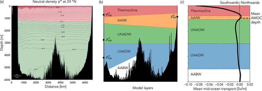
286                                                               E. L. Worthington et al.: 30-year AMOC reconstruction

sponse to anthropogenic forcing (Roberts et al., 2014), which    along the western side of the Mid-Atlantic Ridge. The parti-
the time series is currently too short to detect. Although the   tion between the upper southward and deep southward trans-
AMOC has been well-observed at 26◦ N since 2004, prior           ports defines the strength of the overturning circulation: a
to this, estimates of AMOC strength were restricted to in-       weak AMOC is associated with a greater recirculation within
stances of transatlantic hydrographic sections along 24.5◦ N     the upper layers of the thermocline and weaker deep return
in 1957, 1981, 1992, 1998, and 2004, which provided only         flow; a stronger AMOC is associated with weaker thermo-
snapshots of the overturning circulation strength (Bryden        cline recirculation and stronger deep NADW transport. For
et al., 2005). There are extensive additional hydrographic       an empirical model to more fully represent AMOC dynam-
data around 26◦ N, particularly at the western boundary, but     ics, in particular lower-frequency changes, we suggest that
these are insufficient to reconstruct the AMOC convention-       it must represent these deeper layers. A layered-model in-
ally (Longworth et al., 2011). Due to the limited availability   terpretation of the density structure and the associated water
of hydrographic data, proxies have been used to reconstruct      mass transports is shown in Fig. 1b.
the AMOC time series earlier than 2004.                             Here, we revisit the approach of Longworth et al. (2011)
   In one proxy reconstruction, Frajka-Williams (2015) used      by using linear regression models to represent the AMOC
sea-surface height from satellite altimetry to estimate trans-   and develop the method further to include additional lay-
basin baroclinic transport at 26◦ N between 1993 to 2014. In     ers representative of the deep circulation. Section 2 describes
another, Longworth et al. (2011) used temperature anomaly        how we trained and validated our statistical model using the
at the western boundary as a proxy for geostrophic trans-        RAPID dataset and how we selected historical hydrographic
port within the upper 800 m, or thermocline layer, finding       data to apply to the model. Section 3 describes how these hy-
the temperature anomaly at 400 dbar explained 53 % of the        drographic data were used to create an extended time series
variance in thermocline transport. However, both Longworth       of AMOC strength from 1982 to 2016. In Sects. 4 and 5, we
et al. (2011) and Frajka-Williams (2015) used single-layer       discuss the implications of creating the longest observational
models that do not account for the variable depth structure of   time series of AMOC strength that incorporates variability in
the AMOC in the subtropics.                                      the deep NADW layers and acknowledge the limitations of
   At 26◦ N, the dynamics of the AMOC involve multiple wa-       using an empirical model.
ter masses flowing in opposite directions in different layers,
driven by the changing density structure with depth (Fig. 1a).
Within the permanent thermocline layer, which reaches as         2     Methods
deep as 800 m on the western boundary and 600 m on the
eastern, isopycnals rise towards the eastern boundary, indica-   2.1    Model data
tive of southward flow (Hernández-Guerra et al., 2014). Be-
low the thermocline, isopycnals deepen towards the east, and     Our regression models were trained on RAPID data from
the resulting transport profile (Fig. 1c) shows a small north-   27 May 2006 to 21 February 2017 (Smeed et al., 2017).
ward transport centred around 1000 m sandwiched between          RAPID data are available from 7 April 2004, but we used
southward transports above and below. Although referred to       only data obtained after the collapse of the main western
by RAPID as Antarctic Intermediate Water (AAIW), both            mooring, WB2, between 7 November 2005 and 26 May
AAIW and Mediterranean Water are observed between 700–           2006. McCarthy et al. (2015) describes in detail how RAPID
1600 m on the eastern boundary, with the relative contribu-      measures the AMOC, but it is described briefly here as we
tion of each varying seasonally (Fraile-Nuez et al., 2010;       use both its results and the interim data created during the
Machín and Pelegrí, 2009; Hernández-Guerra et al., 2003).        calculation. AMOC transport at 26◦ N (Tamoc ) is estimated
The transport profile also shows North Atlantic Deep Water       by combining four directly observed components Eq. (1):
(NADW), which has two distinct layers: Upper (UNADW)             Gulf Stream transport within the Florida Straits (Tflo ), which
above 3000 m, primarily formed in the Labrador Sea (Talley       is measured by submarine cables and calibrated by regular
and McCartney, 1982), and Lower (LNADW) below 3000 m,            hydrographic sections (Baringer and Larsen, 2001; Meinen
which has its origins in the overflows from the Nordic Seas      et al., 2010); Ekman transport (Tek ), which here is calculated
(Pickart et al., 2003). Changes observed in one NADW layer       from ERA-Interim reanalysis wind fields; Western Bound-
are not necessarily observed in another. Smeed et al. (2014)     ary Wedge transport (Twbw ), which is obtained from direct
found that the reduction in AMOC strength between 2004           current measurements over the continental slope between the
and 2012 was seen in LNADW but not UNADW, while Bry-             Bahamas and the WB2 mooring at 76.75◦ W; and the internal
den et al. (2005) found that LNADW transport estimated           transport (Tint ), the basin-wide geostrophic transport calcu-
from transatlantic hydrographic sections at 25◦ N decreased      lated from dynamic height profiles described below, relative
from −15 Sv in 1957 to less than −7 Sv in 1998 and 2004 but      to a reference depth of no motion at 4820 dbar. This refer-
the UNADW transport remained between −9 and −12 Sv.              ence depth is selected as the approximate depth of the inter-
Below the NADW layers, there is a small northward transport      face between the southward LNADW and the deeper north-
below 5000 m, Antarctic Bottom Water (AABW), that flows          ward AABW (McCarthy et al., 2015). To the sum of these

Ocean Sci., 17, 285–299, 2021                                                        https://doi.org/10.5194/os-17-285-2021
E. L. Worthington et al.: 30-year AMOC reconstruction                                                                                  287

Figure 1. (a) World Ocean Circulation Experiment (WOCE) North Atlantic A05 section of neutral density γ n (kg m−3 ) at 24◦ N, July or
August 1992. From the WOCE Atlantic Ocean Atlas Vol. 3. (Koltermann et al., 2011). (b) Schematic of four dynamic layers to be represented
within the regression model by density anomalies at the western and eastern boundaries at a depth within each layer. The density anomalies
are represented by the circular markers. (c) Profile of RAPID-estimated mean mid-ocean transport and the resulting northward and southward
layer transports. Mean AMOC depth is around 1100 m.

four components, a depth-dependent external transport (Text )          transport is the sum of the internal, external, and Western
is added to ensure mass is conserved and that there is zero            Boundary Wedge transports. This net southward UMO trans-
net flow across the section. The assumption of zero net flow           port includes the southward gyre recirculation and the north-
holds on timescales longer than 10 d (Kanzow et al., 2007;             ward Antilles Current.
Bryden et al., 2009).                                                               zamoc                     zamoc
                                                                                     Z                         Z
Tamoc (t, z) = Tflo (t, z) + Tek (t, z) + Twbw (t, z)                  Tumo (t) =           Tmo (t, z) dz =           [ Tint (t, z)
+ Tint (t, z) + Text (t, z)                                    (1)      + Twbw (t, z) + Text (t, z) ] dz                                (2)

   The internal geostrophic transport, Tint , is estimated from        2.2   Developing the model
dynamic height profiles. These are created by merging data
from individual moorings to create four profiles for each              For use in the regression models, absolute salinity, conserva-
of the western and eastern boundaries and the western and              tive temperature, and in situ density were calculated from the
eastern sides of the Mid-Atlantic Ridge. For example, at               gridded in situ temperature and practical salinity data created
the western boundary, most data come from instruments de-              during the RAPID calculations. As all AMOC transports are
ployed on the WB2 mooring, but additional data from the                filtered during the RAPID calculation, the same Butterworth
deeper, more eastern WBH2 and WB3 moorings are used to                 10 d, low-pass filter was also applied to the salinity, temper-
cover the full depth. This results in vertical profiles of tem-        ature, and density data; the filtered data were then averaged
perature and salinity with sparse resolution, which are then           from a 12-hourly resolution to a monthly mean. Anomalies of
vertically interpolated using a monthly climatology for each           these data and RAPID-estimated transports were created by
location. As RAPID data are vertically interpolated over a             subtracting the mean between 27 May 2006 and 21 February
pressure grid, depth will henceforth be reported in decibars           2017, and these monthly mean anomalies were used to train
(dbar) rather than metres. These four merged and interpo-              all our regression models.
lated temperature and salinity profiles are used to calculate              We revisited the linear regression made by Longworth
dynamic height (referenced to 4820 dbar), which is then ex-            et al. (2011), an ordinary least-squares (OLS) regression be-
trapolated to the surface using a seasonal climatology.                tween the conservative temperature anomaly at 400 dbar and
   The strength of the AMOC is then the maximum of Tamoc               the thermocline transport anomaly. Longworth et al. (2011)
integrated over depth from the surface, i.e. the maximum of            suggested that increasing southward thermocline transport
the transport streamfunction, and the AMOC depth (zamoc ) is           (a negative transport anomaly) causes more warm water
the depth of that maximum at each time step, usually around            to recirculate close to the western boundary, and so the
1100 m. The upper mid-ocean (UMO) transport (Tumo ) is de-             temperature at any particular depth within the thermocline
fined as the mid-ocean transport (Tmo ) integrated between the         will increase (a positive temperature anomaly). They chose
surface and the AMOC depth Eq. (2), where the mid-ocean                400 dbar as both the mid-point of the thermocline layer and

https://doi.org/10.5194/os-17-285-2021                                                                        Ocean Sci., 17, 285–299, 2021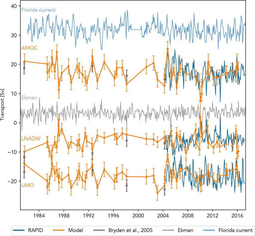
288                                                               E. L. Worthington et al.: 30-year AMOC reconstruction

a depth at which every profile had a sensor deployed within      shows the four explanatory variables – three western and one
50 m. We used 132 monthly mean conservative temperature          eastern boundary density anomalies – representing the ther-
anomalies at 400 dbar from the RAPID western boundary            mocline (ρwbz1 ), AAIW (ρ z2 ), UNADW (ρ z3 ), and LNADW
                                                                                           eb                 wb
profile, compared to their 39 historic CTD (conductivity–          z4
                                                                 (ρwb ) layers. The superscripts z1, z2, z3, and z4 indicate the
temperature–depth) profiles. Our regression, however, shown      anomaly depths to be identified by the algorithm.
in the scatter plot in (Fig. 2a), explained only 20 % of the
variance of the thermocline transport anomaly, compared
                                                                               z1          z2          z3
with 53 % for the original result based on the shorter time      Tumo (t) = α ρwb (t) + β ρeb (t) + γ ρwb (t)
series. To investigate whether the regression fit could be im-        z4
                                                                 + ζ ρwb (t)                                                (3)
proved by using the temperature anomaly from a different
depth, we used an algorithm to repeat the same regression           Initially a model with two explanatory variables represent-
using the conservative temperature anomaly every 20 dbar                                z1 ) and AAIW (ρ z2 ) layers was imple-
                                                                 ing the thermocline (ρwb                 eb
from 220 to 800 dbar, and report at which depth the high-        mented; then variables representing the UNADW (ρwb     z3 ) and
est explained variance, or adjusted R 2 value, was found. The                             z4
                                                                 finally the LNADW (ρwb ) were added. All possible combi-
highest explained variance found by the algorithm was 51 %       nations of density anomaly depths within each layer were
for the regression using the western boundary temperature        used to run the regression to find which combination gave
anomaly at 780 dbar (Fig. 2b). Changing the regression to use    the maximum adjusted R 2 value. For example, for the two-
the density anomaly made very little difference, increasing      layer model, each western boundary density anomaly every
the adjusted R 2 to 0.54, with the anomaly again at 780 dbar.    20 dbar between 220 and 780 dbar was combined in turn with
   We expanded this one-layer model by creating multiple         each eastern boundary density anomaly every 20 dbar be-
linear regression models using two, three, and four explana-     tween 800 and 1080 dbar and regressed against the UMO
tory variables to represent two, three, and four layers re-      transport anomaly. Due to the number of iterations required
spectively, reflective of the water mass and circulation depth   by adding the fourth variable, the western boundary density
structure. We used RAPID-defined layers: the thermocline         anomalies representing the UNADW and LNADW in this
between the surface and 800 dbar; Antarctic Intermediate         model were chosen every 100 dbar rather than every 20.
Water (AAIW) between 800 and 1100 dbar; Upper North At-             The OLS regressions were checked against a number of
lantic Deep Water (UNADW) between 1100 and 3000 dbar;            assumptions that should hold for a linear regression model
and Lower North Atlantic Deep Water (LNADW) between              to be fit for purpose, for example, a known issue for those
3000 and 4820 dbar (Fig. 1b). UMO transport (Tumo ), as          models based on time series is autocorrelation of residuals.
the main contributor to the AMOC, was preferred to ther-         We found that all our OLS models, whether using simple or
mocline transport as the dependent variable for all subse-       multiple linear regression, showed autocorrelation of residu-
quent regression models. Variability of the AMOC is dom-         als, indicated by Durbin–Watson values between 0 and 1. An
inated by the western boundary (Elipot et al., 2014; Bryden      alternate linear regression model was used, the generalised
et al., 2009); and Frajka-Williams et al. (2016) showed strong   least-squares model with autocorrelated errors (GLSARs),
positive correlation between UMO transports and isopycnal        which models autocorrelation of residuals for a given lag
displacements on the western boundary around 820 m and           (McKinney et al., 2019). For each of our models, autocorrela-
negative correlation between LNADW transport and isopyc-         tion was significant for a lag of 1 month, which is consistent
nal displacements on the western boundary between 1500 m         with Smeed et al. (2014), who show that the decorrelation
and the bottom. Western boundary density anomalies were          length scale associated with the AMOC is 40 d.
thus chosen as the independent variables representing each
layer, with the exception of AAIW. The seasonal cycle of         2.3   Evaluating the model
the AMOC is driven largely by seasonality at the eastern
boundary (Chidichimo et al., 2010; Pérez-Hernández et al.,       The simplest model selected by the algorithm, regressing
2015). The annual maximum northward transport at the east-       UMO transport anomaly on the western boundary density
ern boundary and the AMOC occur around October (Vélez-           anomaly at 780 dbar, gives an adjusted R 2 value of only
Belchí et al., 2017) and is driven by changes in the cir-        0.49, shown in the top time series plot (Fig. 3a). This plot
culation of the Canary Current (Casanova-Masjoan et al.,         also shows relatively large model prediction intervals (orange
2020; Hernández-Guerra et al., 2017) and at intermediate         shading), which give the range of UMO transport anomalies
depths (700–1400 dbar) by seasonal changes in the Interme-       that we have 95 % confidence will occur for that combination
diate Poleward Undercurrent (Hernández-Guerra et al., 2017;      of boundary density anomalies. However, adding the eastern
Vélez-Belchí et al., 2017). Eastern boundary density anoma-      boundary density anomaly at 1020 dbar (ρeb 1020 ) increases the

lies have maximum subsurface variability around 1000 dbar                               2
                                                                 maximum adjusted R to 0.74 (Fig. 3b) and reduces the pre-
(Chidichimo et al., 2010), so the AAIW layer was repre-                                          z3 and then the ρ z4 western
                                                                 diction intervals. Adding the ρwb                   wb
sented by an eastern boundary density anomaly between            boundary density anomalies further increases the adjusted R 2
800 and 1100 dbar. The multiple linear regression Eq. (3)        value of the model to 0.76 and 0.78 respectively (Fig. 3c and

Ocean Sci., 17, 285–299, 2021                                                        https://doi.org/10.5194/os-17-285-2021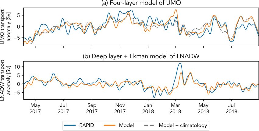
E. L. Worthington et al.: 30-year AMOC reconstruction                                                                               289

Figure 2. Linear regression of the monthly mean RAPID thermocline (0–800 m) transport anomaly on the monthly mean conservative
temperature anomaly at (a) 400 dbar and (b) 780 dbar from the RAPID western boundary profiles. The orange line is the regression equation
for these data; the blue dashed line in (a) shows the equivalent regression from Longworth et al. (2011) for the same data. The Pearson’s
correlation coefficient (r) is shown for each model regression.

d). Although increasing layers from two to three to four does          values well (r = 0.75). It also shows that when the eastern
not increase the adjusted R 2 greatly, it does reduce the stan-        boundary density anomaly at 980 dbar is replaced with a
dard error of the regression from 1.85 Sv for the single-layer         monthly climatology, the trends and variability are also well
model to 1.32, 1.27, and 1.23 Sv for the two-, three-, and             captured (Fig. 4b, r = 0.71). The reason that a climatology
four-layer models. The algorithm also selects slightly differ-         was tested will be discussed in Sect. 2.5 when we describe
ent density anomaly depths for these last two regressions:             the selection of historical hydrographic data.
720, 980, and 1200 dbar when three variables are used and                 Our model was trained on monthly mean density anoma-
740, 980, 1200, and 3000 dbar when all four are included.              lies but was to be used with hydrographic data from much
As using explanatory variables to represent all four layers            shorter periods of a day or two. To evaluate how well these
gives a regression model that explains the greatest variance           “snapshot” profiles represented the longer periods, we sim-
in the UMO transport anomaly and has the lowest standard               ulated them by randomly selected 20 single points from the
error, it was selected to apply to the historical hydrographic         7961 available 12-hourly values from the most recent RAPID
data. The resulting multiple linear regression Eq. (4) shows           data. These were applied to the model and the predicted
the depths chosen for each of the four density anomalies by            UMO compared to the observed monthly mean UMO for
the algorithm and the coefficients for each.                           the same time, with the model error being the difference be-
                                                                       tween the two. Bootstrapping the model prediction showed
                                                                       that around 65 % of the observed UMO values were within
             740         980         1200         3000
Tumo = 40.5 ρwb  − 98.6 ρeb  + 46.7 ρwb   + 46.8 ρwb          (4)      the prediction interval of the corresponding model UMO.
                                                                       The standard deviation of the bootstrapped model errors was
   The selected model was cross-validated using a 30 : 70 %            2.8 Sv.
training / testing split of the RAPID data, to investigate its            The CTD profiles to be applied to the regression model
suitability for predicting over a period much longer than              to estimate UMO transport occur at irregular intervals, so
the almost 11 years of RAPID data used to train the full               to allow comparisons between periods, we calculated the
model. The two cross-validation models, trained using the              mean transport anomalies for a given time window. Addition-
first and last 30 % of the RAPID data, both predict UMO                ally, we calculated the weighted rolling mean for the trans-
transport anomalies for the remaining 70 % that agree well             port anomalies with the RAPID annual cycle removed, using
with the observations (r = 0.88). The full model was then              a Gaussian distribution over the same time window. Since
tested against new RAPID data not used to train it, made               Smeed et al. (2014) calculated means for two 4-year peri-
available following the most recent expedition and covering            ods – 2004–2008 and 2008–2012 – from April to March, we
the period from February 2017 to November 2018 (Smeed                  used the same 4-year window for both the period mean and
et al., 2019). The model-predicted UMO transport anomaly               weighted rolling mean to allow a direct comparison. Since
shown in Fig. 4a shows that it reproduces the trends and vari-         the UMO is a transport specific to RAPID, we also esti-
ability, although not always the magnitude, of the observed

https://doi.org/10.5194/os-17-285-2021                                                                Ocean Sci., 17, 285–299, 2021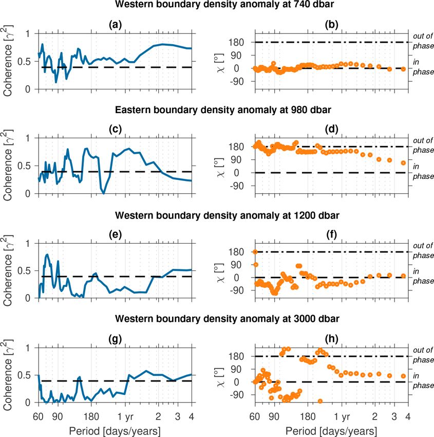
290                                                                      E. L. Worthington et al.: 30-year AMOC reconstruction

Figure 3. Comparison of UMO transport anomaly predicted by GLSAR(1) regression models using one to four layers with the UMO
transport anomaly observed by RAPID. The layers represented by the regression-independent variables are shown above each plot, and the
model R 2 value, adjusted for the degrees of freedom of each model, and standard error of the regression are shown to the right. The orange
shading around each model prediction line shows the 95 % prediction interval. The blue shading around the observed transport shows the
1.5 Sv uncertainty estimated by McCarthy et al. (2015)

mated the AMOC by adding the model-derived UMO trans-                   periods from 120 d to 4 years. The highest significance oc-
port to the monthly mean Florida Current and Ekman trans-               curs for periods of around 65 d and 2–3 years (Fig. 5a) and is
port anomalies for the same date. The Florida Current data              in phase at all periods (Fig. 5b). The eastern boundary den-
were the Western Boundary Time Series daily mean trans-                 sity anomaly at 980 dbar, representing the AAIW water mass
port estimates from submarine cable voltage, and the Ekman              transport, shows significant coherence for periods between
data were the same ERA-interim reanalysis-derived Ekman                 100 and 120 d, 150 and 200 d, and 280 d and 1.5 years, with
transports as used by RAPID. The Florida Current data have              the strongest coherence at around 160 d and just over 1 year
a gap between 22 October 1998 and 19 June 2000. There                   (Fig. 5c). The coherence for this variable is out of phase for
were no selected hydrographic profiles during this gap, but             most periods with significant coherence, (Fig. 5d), which is
this period was filled with the time series mean to allow the           consistent with its negative coefficient. The western bound-
4-year mean and weighted rolling mean to be calculated for              ary density anomaly at 1200 dbar, representing the UNADW
the Florida Current transport. To give overall transports, the          water mass transport, shows significant coherence for periods
relevant mean transports from the RAPID data used to train              between 67 and 80 d and around 90 d and to a lesser extent
the model (27 May 2006 to 21 February 2017) were added to               around 200 d (Fig. 5e). The significant coherence is approxi-
the 4-year and rolling mean anomalies.                                  mately in phase, with the observed UMO transport anomaly
   To evaluate the co-variability of the density anomaly se-            lagging the 1200 dbar density anomaly slightly (Fig. 5f). Fi-
lected to represent each water mass transport and the ob-               nally, the western boundary density anomaly at 3000 dbar,
served UMO transport anomaly, we determined the coher-                  representing the LNADW water mass transport, shows sig-
ence between them using a multi-taper spectrum follow-                  nificant coherence only for periods at just under 140 d and
ing Percival and Walden (1998). This method reduces spec-               between just over 1 year, or 400 d (Fig. 5g), and just over 2.5
tral leakage while minimising the data loss associated with             years, or 990 d. For this latter period, the co-variability is also
other tapers. The number of tapers used was K = 2p − 1,                 approximately in phase, with the 3000 dbar density anomaly
where p = 4 and the 95 % confidence level was given by                  lagging the UMO transport anomaly slightly (Fig. 5h).
1 − 0.051/(K−1) . The western boundary density anomaly at
740 dbar, which represents the thermocline water mass trans-
port, shows significant coherence with the observed UMO
transport at periods of around 65, 75, and 95 d and then at all

Ocean Sci., 17, 285–299, 2021                                                                 https://doi.org/10.5194/os-17-285-2021
E. L. Worthington et al.: 30-year AMOC reconstruction                                                                             291

Figure 4. (a) UMO transport anomaly estimated from the most recent RAPID observations (blue) compared to the UMO transport anomaly
predicted by the four-layer regression model (orange) using density anomalies derived from the same RAPID data. The RAPID data were
12-hourly and 10 d filtered. The dashed grey line shows the model prediction where the eastern boundary density anomaly at 980 dbar is
replaced by a monthly climatology. (b) LNADW transport anomaly estimated from the most recent RAPID observations (blue) compared to
the LNADW transport anomaly predicted by the regression model combining the western boundary density anomaly at 3040 dbar (orange)
derived from the same RAPID data and the Ekman transport.

2.4   An additional model: reconstructing Lower North
      Atlantic Deep Water
                                                                                     3040
                                                                     Tlnadw = −175.9ρwb   − 0.4 Tekman                             (5)
The importance of the LNADW in the AMOC decline com-
pared to the UNADW (Smeed et al., 2018) suggested an                    This model was also tested using the RAPID data between
additional linear regression model between the LNADW                 February 2017 to November 2018, and the model-predicted
transport anomaly and two independent variables: a western           LNADW transport anomaly shown in Fig. 4b shows that
boundary density anomaly at a depth within the LNADW                 it compares well with the RAPID-observed equivalent (r =
layer and the Ekman transport anomaly. The Ekman trans-              0.73). The hydrographic profiles selected for use in the UMO
port is included in the model as Frajka-Williams et al. (2016)       empirical model were also applied to this LNADW model
found that LNADW transport showed a deep baroclinic re-              and the 4-year and weighted rolling means calculated using
sponse to changes in Ekman transport. We applied a similar           the same windows.
algorithm to the UMO regression model, repeating the re-
                                                                     2.5   Selecting historical hydrographic data
gression for the deep density anomaly every 20 dbar between
3000 and 4820 dbar and reporting the maximum explained               As Longworth et al. (2011) documented, between 1980 and
variance.                                                            2017 there are many more hydrographic profiles close to
   For the LNADW linear regression, the algorithm selected           the western boundary than the eastern. Since the eastern
the western boundary density anomaly at 3040 dbar, close to          boundary density anomaly shows strong seasonal variabil-
the boundary between the Upper and Lower North Atlantic              ity (Pérez-Hernández et al., 2015; Chidichimo et al., 2010),
Deep Water layers at 3000 dbar. The resulting linear regres-         replacing it in the model with a monthly climatology from
sion Eq. (5) has an adjusted R 2 value of 0.75 and a stan-           the RAPID eastern boundary data, as described in the previ-
dard error of 0.94 Sv, and the coefficients show that a positive     ous Sect. 2.3, allows us to use all available western boundary
anomaly in LNADW transport is associated with both a nega-           profiles, although at the cost of losing a little of the explained
tive density anomaly and negative Ekman transport anomaly.           UMO transport variance.
This means that a reduction in the deep southward LNADW                 Historical hydrographic data were obtained from the
flow is linked to lower-density water at 3040 dbar, which we         World Ocean Database 2018 (WOD2018) (Boyer et al.,
would expect with a reduction in overturning. The inverse            2018) and from the datasets processed by Longworth et al.
relation between LNADW and Ekman transports reflects the             (2011), with duplicate data removed. Data were selected ini-
statistically significant inverse correlation (r = −0.58) found      tially based on a region defined by latitude and longitude
by Frajka-Williams et al. (2016) between the two transports.         from 24 to 27◦ N and from 75 to 77.5◦ W. CTD profiles were
                                                                     then grouped by date, with a date group defined as sepa-
                                                                     rated by 3 d or more. From each group, we selected profiles

https://doi.org/10.5194/os-17-285-2021                                                              Ocean Sci., 17, 285–299, 2021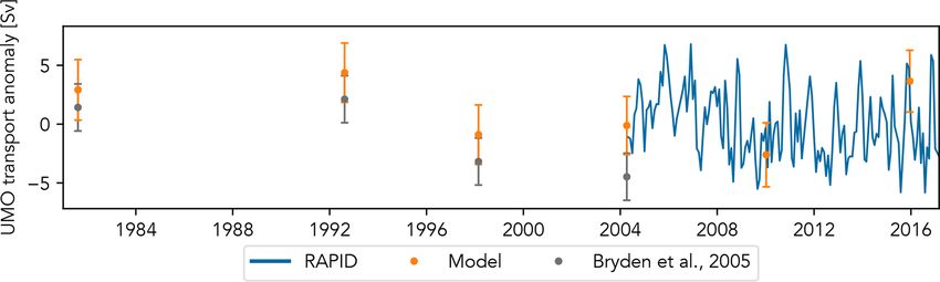
292                                                                      E. L. Worthington et al.: 30-year AMOC reconstruction

Figure 5. Multi-taper spectrum coherence (a, c, e, g) and phase relationship (b, d, f, h) between the UMO transport anomaly observed by
RAPID and the density anomaly that is each independent variable in the linear regression. Significance of coherence (95 % confidence) is
indicated by the black dashed horizontal line in the left-hand panels. The horizontal black dashed lines in the right-hand panels show where
the time series are exactly in phase and exactly 180◦ out of phase.

based on similarity of distance from the continental slope to             3000 . Thus between one and three CTD profiles are selected
                                                                        ρwb
the west as the RAPID WB2 and WBH2 moorings. We jus-                    from each group to use in the model and merged if required.
tify this as the AMOC shows meridional coherence of buoy-               The two regional plans in Fig. 6, which compare all available
ancy anomalies within 100 km, and variability at the west-              CTD profiles and those selected for use in the model, show
ern boundary increases with distance from it (Kanzow et al.,            that the majority were located close to the RAPID western
2009). The RAPID western boundary profile that the model                boundary mooring array.
is based on uses the WB2 mooring for measurements down
to around 3850 dbar and then the WBH2 and WB3 moorings
below this. The distance from each mooring to the continen-             3   Applying the model to historical hydrographic data
tal slope was calculated at the depths of the western bound-
ary density anomalies that the algorithm selected. The same             Initially, we used the western boundary density anomalies
was done for each CTD profile. Then, for the profiles within            derived from the transatlantic sections at 24.5◦ N from 1981,
each group, those with the most similar distance for each               1992, 1998, 2004, 2010, and 2015 to estimate the UMO
depth were selected. For example, for the density anomaly               transport anomaly using the four-layer regression model. The
  740 , the WB2 mooring is 13.8 km from the continental slope
ρwb                                                                     error bars show the model prediction interval, which gives
at 740 dbar. If there are five CTD profiles within the group,           the range of UMO transport anomalies that we have 95 %
with distances from the slope at 740 dbar of 9.8, 12.4, 15.0,           confidence will occur for that combination of boundary den-
18.9, and 27.5 km, then the profile that is 12.4 km away is se-         sity anomalies. The uncertainty for the 1957 section model
lected. The same is done for the density anomalies ρwb1200 and          estimate was much larger than for the later section, and since
                                                                        no suitable hydrographic data before 1981 were available, it

Ocean Sci., 17, 285–299, 2021                                                                 https://doi.org/10.5194/os-17-285-2021
E. L. Worthington et al.: 30-year AMOC reconstruction 293 Figure 6. (a) All CTD profiles from the World Ocean Database 2018 in the region shown, compared with (b) those selected as being the most similar distance from the western boundary as the WB2 and WBH2 RAPID moorings. is omitted from our results. The sections from 1981, 1992, WB2 mooring failure of late 2005 to early 2006, when the 1998 and 2004 were used by Bryden et al. (2005) to re- model estimates a stronger southward UMO than was ob- construct the AMOC fully, and Fig. 7 shows generally very served by RAPID. good agreement between the model and Bryden et al. (2005) The model-estimated AMOC transports shown in Fig. 8 AMOC estimates. Only the 2004 estimate from Bryden et al. also agree well with the equivalent estimates from Bryden (2005) is not within the model’s prediction interval; however et al. (2005), with the exception of 1998, where their esti- the model 2004 estimate appears to be in better agreement mate of 16.1 Sv is just outside the model upper uncertainty with the RAPID observations. The model UMO estimates for of 15.3 Sv. It should be noted, however, that Bryden et al. 2010 and 2015 are also consistent with the RAPID UMO, (2005) used constant values for both Florida Current and Ek- reflecting the large downturn between late 2009 and early man transports, whereas we used monthly mean values based 2010 and a peak in 2015. The model consistently predicts a on observations. The magnitude and trends of the RAPID stronger AMOC than Bryden et al. (2005), with mean and observations are also captured well by the model estimates maximum differences of 2.6 and 4.4 Sv. from CTD profiles taken during the same period. Includ- When the model is applied to western boundary density ing the monthly mean Ekman transport allows the model to anomalies from the selected hydrographic profiles, together capture the 2009–2010 downturn well, although the profiles with the eastern boundary climatology, the resolution of the from November 2009 and October 2010 give the only model UMO time series in Fig. 8 is sufficient to show decadal AMOC transports sufficiently weak to be outside the stan- and multi-annual variability. The standard deviation of the dard deviation of the RAPID monthly mean anomalies of RAPID monthly mean anomalies is ± 2.9 Sv, and the UMO ± 2.4 Sv. Prior to 2004, the model estimates the AMOC to transport anomaly estimated by the model is stronger south- be weaker and outside the standard deviation in March of ward than this in May 1985, March 1989, June 1993, Febru- 1987 and 1989, September 1991, June 1993, February 1998, ary 2003, and March 2004, with each anomaly lower than and March 2004, although none reach the magnitude of the −3.3 Sv. This is stronger than any negative anomaly pre- 2009–2010 downturn, with the weakest AMOC anomaly of dicted by the model during the RAPID period. The UMO −5.5 Sv seen in March 1987. The strongest model AMOC is weaker southward than the RAPID standard deviation anomaly of 8.4 Sv is seen on 2 October 2004, which is very in September 1981, February 1986, July and August 1992, close to the RAPID mean anomaly for September 2004 of October 2004, and October and December 2015, with the 8.7 Sv. The AMOC anomaly was also over 2.4 Sv for 11 pro- anomaly again being greater than 3.5 Sv with the exception files during the 23 years prior to the start of RAPID and 4 of July 1992. When compared directly to the RAPID obser- profiles during the 13 years of RAPID observations shown vations, the model predictions generally agree well with the here. overall trends, with one notable exception during the RAPID https://doi.org/10.5194/os-17-285-2021 Ocean Sci., 17, 285–299, 2021
294 E. L. Worthington et al.: 30-year AMOC reconstruction
Figure 7. UMO transport anomaly estimated by the empirical model using density anomalies from six transatlantic hydrographic sections,
compared to estimates from Bryden et al. (2005) and RAPID. The uncertainties shown for the model-derived values are the model’s prediction
intervals; the Bryden et al. (2005) uncertainty is 2 Sv.
Compared to the LNADW estimates from transatlantic 2008 and 2008–2012 and 1.5 Sv for 2012–2016. The 2000–
sections made by Bryden et al. (2005), the model predictions 2004 mean reflects the UMO downturn, with the lowest 4-
get closer with each subsequent section from 1981 to 2004. year mean value of 14.8 Sv, again lower than the 2008–2012
The model-estimated transports are all more positive than mean AMOC transport for both model and RAPID by 0.4
those of Bryden et al. (2005) with the exception of 2004. The and 1.1 Sv respectively.
LNADW transport estimated by the model for April 2004 The 4-year LNADW rolling mean suggests a non-
differs from that estimated by Bryden et al. (2005) by only monotonic weakening trend in the southward deep return
0.3 Sv and from the observed RAPID LNADW transport by flow between 1985 and 1999, from 8.5 Sv southwards in
less than 0.1 Sv. The model LNADW transports prior to 2004 1985 decreasing to 3.8 Sv southwards in 1999. The rolling 4-
show a weakening in 1987 to +1 Sv, almost as weak as the year mean then varies by less than 0.6 Sv between 2000 and
observed RAPID monthly mean LNADW transports of 1.3, 2008, then weakens again to between 4.6 and 4.3 Sv south-
1.0, and 1.6 Sv in January and December 2010 and March wards in 2009 and 2010 respectively before increasing in
2013 respectively. The model LNADW transports post-2004 strength again to a maximum southward transport of 7.7 Sv
are in reasonable agreement with RAPID trends although in 2013. RAPID mean southward values for 2004–2008 and
tend to over- or underestimate the strength. The observed 2008–2012 are stronger than the model by 0.9 and 0.3 Sv re-
weakening of southward LNADW flow in 2010 is captured spectively, but for 2012–2016 they are 1.8 Sv weaker. The
well, with the model LNADW showing a strong positive greater disagreements between model and RAPID mean val-
anomaly. ues for AMOC and LNADW transports may be due to the
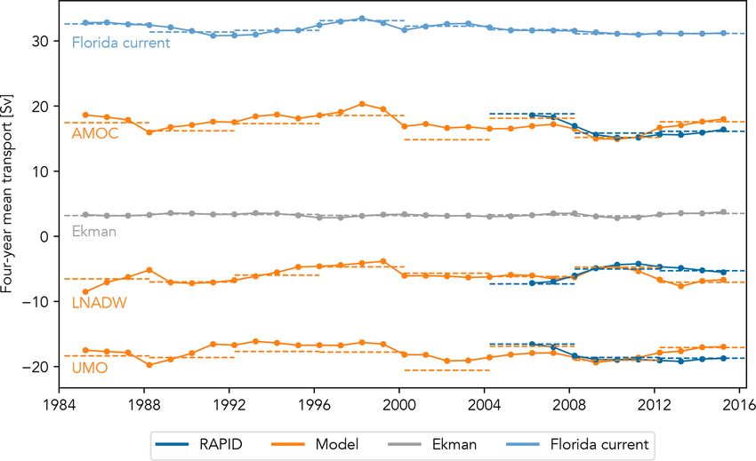
The 4-year mean transports in Fig. 9 show that between additional smoothing caused by using monthly mean Ekman
1984 and 2000, the UMO strength was within 0.6 Sv of the transport to estimate them rather than the 10 d filtered val-
RAPID mean UMO of −18.3 Sv, taken for the period used ues used by RAPID. None of the model-estimated UMO,
to create the model. The 4-year means begin from 1984 as AMOC, or LNADW transports show an overall trend.
prior to this there is only a single profile. The period with
the strongest southward 4-year mean UMO is 2000–2004 at
−20.6 Sv, lower than the RAPID reduced period of 2008– 4 Discussion
2012 and 2012–2016 when the mean UMO transports were
−18.6 and −18.7 Sv respectively; however the error for the Although the AMOC has been well-observed since 2004 by
model mean is 4.4 Sv. The 4-year model mean UMO trans- RAPID, before this, estimates of AMOC transport were re-
port also compares well to the RAPID equivalent for 2004– stricted to approximately decadal transatlantic sections. It
2008 and 2008–2012, each differing by only 0.4 Sv. The has been estimated that a time series of at least 60 years
model mean UMO for 2012–2017 is however 1.6 Sv higher is necessary to detect long-term change in the AMOC due
than the RAPID mean. The Gaussian-weighted 4-year rolling to anthropogenic global warming (Baehr et al., 2008), so
mean also suggests that the multi-year UMO variability was extending the AMOC record into the past is crucial. Al-
low during the 1990s, followed by a period of strengthened though proxies have been used to extend AMOC estimates
southward transport in the early 2000s. It also suggests a earlier, these use one, or at most two, layers to represent
weakening of southward UMO transport from 2012 not seen AMOC dynamics (Longworth et al., 2011; Frajka-Williams,
in the observations. 2015). However, Baehr et al. (2007) showed that deep den-
The 4-year mean AMOC transports show slightly more sity measurements were important in reducing the length of
variability than the UMO, and agree slightly less well with the time series required to detect anthropogenic change, and
the RAPID 4-year mean values, differing by 0.7 Sv for 2004– single-layer models neglect this. In this study, we showed
that an empirical regression model applied to historical hy-
Ocean Sci., 17, 285–299, 2021 https://doi.org/10.5194/os-17-285-2021E. L. Worthington et al.: 30-year AMOC reconstruction 295 Figure 8. UMO and LNADW transports estimated by empirical models using density anomalies from hydrographic CTD profiles, compared to estimates from RAPID and Bryden et al. (2005). The 980 dbar eastern boundary density anomaly for the UMO model was replaced by RAPID monthly climatology. The monthly mean Florida Current and Ekman transports are also shown and were added to the UMO model-estimated transports to give the estimated AMOC transport. drographic data could be used to improve the resolution of (2015), which is implicitly single-layer, estimated the mean the UMO and hence AMOC transport estimates compared to UMO for 1993–2003 and 2004–2014 to vary by only 0.1 Sv. the sparse transatlantic sections. In addition, by representing By contrast, our model estimated the same 11-year means the deep return layers of the AMOC, the model could capture as −19.0 and −18.2 Sv, a difference of 0.8 Sv. The 11-year lower-frequency changes missed by other proxy models. mean for 1982–1992 was −18.1 Sv, showing that our four- To develop this empirical model of the AMOC, we re- layer model captures more of a change in the UMO. The gressed UMO transport on western boundary density anoma- model mean UMO transport for 2004–2014 of −18.2 Sv also lies within each of the thermocline, UNADW, and LNADW agrees well with the RAPID equivalent of −17.9 Sv. The im- layers and an eastern boundary climatology within the AAIW portance of representing the deep layers can be seen in re- layer, using an algorithm to select the best depth for each den- peating the predictions using the two- and three-layer models sity anomaly. The selected model was then applied to histor- described earlier. The two-level model representing the upper ical hydrographic CTD profiles to predict UMO and hence two layers gives decadal mean differences in UMO trans- AMOC transport strength between 1981 and 2016, at ap- port of 0.3 Sv, while adding the upper deep layer increases proximately annual resolution. This resolution is sufficient the mean UMO for 1982–1992, 1993–2003, and 2004–2014 to show pentadal to decadal variability, with a model uncer- to −18.3, −18.7, and −18.1 Sv respectively, a difference of tainty of around ± 2.5 Sv. 0.6 Sv. The AMOC proxy from Frajka-Williams (2015) had There is no overall trend in either AMOC or UMO mean transports for 1993–2003 and 2004–2014 of 18.3 and as estimated by the model, but 4-year means, following 17.1 Sv, while the RAPID mean AMOC transport for 2004– Smeed et al. (2018), suggest that there were stronger south- 2014 was 16.9 Sv. The 11-year mean AMOC transports were ward UMO and stronger northward AMOC transports be- predicted by our model as 17.8, 17.4, and 15.9 Sv for 1982– tween 2000 and 2004 than at any time observed by RAPID. 1992, 1993–2003, and 2004–2014 respectively, again show- The sea-surface height model developed by Frajka-Williams ing greater variability than the altimetry-based results. https://doi.org/10.5194/os-17-285-2021 Ocean Sci., 17, 285–299, 2021
296                                                                    E. L. Worthington et al.: 30-year AMOC reconstruction

Figure 9. Four-year means (dashed lines) from 1984 to 2016 and the Gaussian-weighted rolling mean with a 4-year window (solid line),
with the markers showing the mid-point, for AMOC, LNADW, and UMO transports estimated by the relevant regression models (orange)
and from RAPID observations (dark blue). The 4-year and rolling means for Florida Current (light blue) and Ekman (dark grey) transports
are also shown.

   In addition to the four-layer UMO–AMOC model, we also              5   Conclusions
created a similar model regressing LNADW transport on the
deep western boundary density anomaly at 3040 dbar and
Ekman transport. The 4-year mean LNADW transport es-                  In conclusion, this study shows that the dynamics of the
timates from the same hydrographic profiles show lower-               AMOC can be represented by an empirical linear regres-
frequency variability than the UMO–AMOC, suggesting the               sion model using boundary density anomalies as proxies
deep southward return flow was strong throughout the late             for water mass layer transports. More than one layer, rep-
1980s and 1990s, weakening towards 2000. The 4-year mean              resented by boundary density anomalies, is required to cap-
is also weak during the observed AMOC downturn of 2008–               ture lower-frequency changes to UMO transport. Deep den-
2012. The rolling 4-year means for all three transports reflect       sity anomalies combined with Ekman transport are success-
the changes observed by RAPID well, with decreasing north-            ful in reconstructing LNADW transport, the deepest limb of
ward AMOC transport and decreasing deep southward return              the AMOC in the subtropical North Atlantic. Previous prox-
flow balanced by an increase in southward gyre recirculation          ies for AMOC or UMO at 26◦ N that rely on single-layer dy-
(Smeed et al., 2018).                                                 namics (e.g. Frajka-Williams, 2015; Longworth et al., 2011)
   Although this model increases the temporal resolution of           cannot capture this low-frequency variability. This is also the
AMOC estimates, the resolution is still coarse compared to            case for similar reconstructions at other latitudes, for exam-
RAPID and the time intervals between profiles are inconsis-           ple Willis (2010). Single-layer dynamics are also fundamen-
tent. The longest period where no interval is greater than 1          tal to estimates of the AMOC that use fixed levels of no mo-
year is October 1988 to July 1994. There are only two inter-          tion such as the MOVE (Meridional Overturning Variabil-
vals longer than 2 years: September 1981 to April 1985 and            ity Experiment) array (Send et al., 2011) or inverted echo
February 1998 to April 2001. The longest interval is 1328 d           sounders (see McCarthy et al. (2020) for details). We have
and the mean is 210 d. Although this resolution is sufficient         shown the importance of the inclusion of deep density mea-
to show multi-year variability, as shown by the 4-year means,         surements in AMOC reconstructions and believe these to be
the length of some of the sampling intervals and their incon-         key to identifying the fingerprint of anthropogenic AMOC
sistency means the model cannot show interannual variability          change (e.g. Baehr et al., 2008).
reliably.                                                                Our model, applied to historical hydrographic data, has in-
                                                                      creased the resolution of the observed AMOC between 1981
                                                                      and 2004 from approximately decadal to approximately an-
                                                                      nual, and in doing so we have shown decadal and 4-yearly
                                                                      variability of the AMOC and its associated layer transports.
                                                                      The result is the creation of an AMOC time series extend-

Ocean Sci., 17, 285–299, 2021                                                              https://doi.org/10.5194/os-17-285-2021
E. L. Worthington et al.: 30-year AMOC reconstruction 297
ing over 3 decades, including for the first time deep density with analysis. ELW prepared the paper with contributions from all
anomalies in an AMOC reconstruction. co-authors.
Our model has not revealed an AMOC decline indicative
of anthropogenic climate change (Stocker et al., 2013) nor
the long-term decline reported in sea-surface-temperature- Competing interests. The authors declare that they have no conflict
based reconstructions of the AMOC (Caesar et al., 2018). of interest.
It has accurately reproduced the variability observed in the
RAPID data, showing that the downturn between 2008 and
2012 (McCarthy et al., 2012) marked not only the weakest Acknowledgements. ELW was supported by the Natural Environ-
mental Research Council (grant number NE/L002531/1). GM was
AMOC of the RAPID era but the weakest AMOC since the
supported by the A4 project (grant aid agreement PBA/CC/18/01)
mid-1980s. Since this minimum, the strength of the AMOC supported by the Irish Marine Institute under the Marine Research
has recovered in line with observations from the RAPID ar- Programme funded by the Irish Government, co-financed by the
ray (Moat et al., 2020). In fact, according to our model, ERDF. The authors thank the many officers, crews, and technicians
southward flowing LNADW has regained a vigour not seen who helped to collect these data.
since the 1980s. Recent cold and fresh anomalies in the sur- The authors would like to thank Penny Holliday for her feedback
face of the North Atlantic subpolar gyre seemed to indicate and support of the study and Eleanor Frajka-Williams for the code
a return to a cool Atlantic phase associated with a weak used to produce the coherence and phase relationship plots in Fig. 5,
AMOC (Frajka-Williams et al., 2017). However, a weakened which is based on the jLab software package (Lilly, 2017).
AMOC was not the primary cause of these anomalies (Josey The authors would also like to thank the two anonymous review-
et al., 2018; Holliday et al., 2020). Whether a restrength- ers whose comments and suggestions helped improve and clarify
this paper.
ened AMOC will ultimately have a strong impact on Atlantic
climate such as was believed to have occurred in the 1990s
(Robson et al., 2012) remains to be seen.
Financial support. This research has been supported by the Natu-
ral Environment Research Council (grant nos. NE/L002531/1 and
NE/N018044/1), EU Horizon 2020 project Blue-Action (grant no.
Code availability. Original code for this analysis was written in 727852), the National Science Foundation (grant no. 1332978),
Python and is available on request to the corresponding author. the National Oceanic and Atmospheric Administration (grant no.
100007298), the European Regional Development Fund (grant
no. PBA/CC/18/01), and the Climate Program Office (grant no.
Data availability. Data from the RAPID AMOC mon- 100007298).
itoring project are funded by the Natural Environ-
ment Research Council and are freely available from
http://rapid.ac.uk/rapidmoc/rapid_data/datadl.php (last access: Review statement. This paper was edited by Katsuro Katsumata
29 September 2020; https://doi.org/10.5285/5ACFD143- and reviewed by two anonymous referees.
1104-7B58-E053-6C86ABC0D94B, Smeed et al., 2017;
https://doi.org/10.5285/8cd7e7bb-9a20-05d8-e053-6c86abc012c2,
Smeed et al., 2019). The Florida Current cable and
section data are made freely available on the Atlantic
Oceanographic and Meteorological Laboratory web page
References
(https://www.aoml.noaa.gov/phod/floridacurrent/, last access:
2 November 2020) and are funded by the DOC-NOAA Cli-
Baehr, J., Haak, H., Alderson, S., Cunningham, S. A.,
mate Program Office – Ocean Observing and Monitoring
Jungclaus, J. H., and Marotzke, J.: Timely Detection
Division. The World Ocean Database (WOD) is an NCEI
of Changes in the Meridional Overturning Circulation
product and an IODE (International Oceanographic Data
at 26◦ N in the Atlantic, J. Climate, 20, 5827–5841,
and Information Exchange) project. The work is funded in
https://doi.org/10.1175/2007JCLI1686.1, 2007.
partnership with the NOAA OAR Ocean Observing and
Baehr, J., Keller, K., and Marotzke, J.: Detecting Potential Changes
Monitoring Division. WOD2018 data are freely available at
in the Meridional Overturning Circulation at 26◦ N in the At-
https://www.nodc.noaa.gov/OC5/WOD/pr_wod.html (Boyer et al.,
lantic, Clim. Change, 91, 11–27, https://doi.org/10.1007/s10584-
2018). The ECMWF ERA-Interim reanalysis data are freely
006-9153-z, 2008.
available at https://apps.ecmwf.int/datasets/ (last access: 23 June
Baringer, M. O. and Larsen, J. C.: Sixteen Years of Florida Cur-
2020).
rent Transport at 27◦ N, Geophys. Res. Lett., 28, 3179–3182,
https://doi.org/10.1029/2001GL013246, 2001.
Boyer, T. P., Antonov, J. I., Baranova, O. K., Coleman, C., Gar-
Author contributions. ELW and GDM conceived and designed the cia, H. E., Grodsky, A., Johnson, D. R., Locarnini, R., Mishonov,
study. Analysis was carried out by ELW under supervision by R. A., O’Brien, T., Paver, C., Reagan, J., Seidov, D., Smolyar,
GDM, JVM, and RM. BIM and DAS provided software and helped I. V., and Zweng, M.: NCEI Standard Product: World Ocean
Database (WOD), NOAA National Centers for Environmental
https://doi.org/10.5194/os-17-285-2021 Ocean Sci., 17, 285–299, 2021298 E. L. Worthington et al.: 30-year AMOC reconstruction Information, Dataset, available at: https://www.nodc.noaa.gov/ Hernández-Guerra, A., Pelegrí, J. L., Fraile-Nuez, E., Benítez- OC5/WOD/pr_wod.html (last access: 16 April 2020), 2018. Barrios, V., Emelianov, M., Pérez-Hernández, M. D., Bryden, H. L., Longworth, H. R., and Cunningham, S. A.: Slowing and Vélez-Belchí, P.: Meridional Overturning Trans- of the Atlantic Meridional Overturning Circulation at 25◦ N, Na- ports at 7.5N and 24.5N in the Atlantic Ocean during ture, 438, 655–657, https://doi.org/10.1038/nature04385, 2005. 1992–93 and 2010–11, Progr. Oceanogr., 128, 98–114, Bryden, H. L., Mujahid, A., Cunningham, S. A., and Kanzow, T.: https://doi.org/10.1016/j.pocean.2014.08.016, 2014. Adjustment of the basin-scale circulation at 26◦ N to variations Hernández-Guerra, A., Espino-Falcón, E., Vélez-Belchí, P., Dolores in Gulf Stream, deep western boundary current and Ekman trans- Pérez-Hernández, M., Martínez-Marrero, A., and Cana, L.: Re- ports as observed by the Rapid array, Ocean Sci., 5, 421–433, circulation of the Canary Current in Fall 2014, J. Marine Syst., https://doi.org/10.5194/os-5-421-2009, 2009. 174, 25–39, https://doi.org/10.1016/j.jmarsys.2017.04.002, Caesar, L., Rahmstorf, S., Robinson, A., Feulner, G., and 2017. Saba, V.: Observed Fingerprint of a Weakening Atlantic Holliday, N. P., Bersch, M., Berx, B., Chafik, L., Cunningham, S., Ocean Overturning Circulation, Nature, 556, 191–196, Florindo-López, C., Hátún, H., Johns, W., Josey, S. A., Larsen, https://doi.org/10.1038/s41586-018-0006-5, 2018. K. M. H., Mulet, S., Oltmanns, M., Reverdin, G., Rossby, T., Casanova-Masjoan, M., Pérez-Hernández, M. D., Vélez-Belchí, P., Thierry, V., Valdimarsson, H., and Yashayaev, I.: Ocean Cir- Cana, L., and Hernández-Guerra, A.: Variability of the Canary culation Causes the Largest Freshening Event for 120 Years Current Diagnosed by Inverse Box Models, J. Geophys. Res.- in Eastern Subpolar North Atlantic, Nat. Commun., 11, 585, Oceans, 125, https://doi.org/10.1029/2020JC016199, 2020. https://doi.org/10.1038/s41467-020-14474-y, 2020. Chidichimo, M. P., Kanzow, T., Cunningham, S. A., Johns, W. E., Johns, W. E., Baringer, M. O., Beal, L. M., Cunningham, S. A., and Marotzke, J.: The contribution of eastern-boundary density Kanzow, T., Bryden, H. L., Hirschi, J. J., Marotzke, J., Meinen, variations to the Atlantic meridional overturning circulation at C. S., Shaw, B., and Curry, R.: Continuous, Array-Based Esti- 26.5◦ N, Ocean Sci., 6, 475–490, https://doi.org/10.5194/os-6- mates of Atlantic Ocean Heat Transport at 26.5◦ N, J. Climate, 475-2010, 2010. 24, 2429–2449, https://doi.org/10.1175/2010JCLI3997.1, 2011. Cunningham, S. A., Kanzow, T., Rayner, D., Baringer, M. O., Johns, Josey, S. A., Hirschi, J. J.-M., Sinha, B., Duchez, A., Grist, W. E., Marotzke, J., Longworth, H. R., Grant, E. M., Hirschi, J. J. P., and Marsh, R.: The Recent Atlantic Cold Anomaly: J.-M., Beal, L. M., Meinen, C. S., and Bryden, H. L.: Temporal Causes, Consequences, and Related Phenomena, Annu. Rev. Variability of the Atlantic Meridional Overturning Circulation at Mar. Sci., 10, 475–501, https://doi.org/10.1146/annurev-marine- 26.5◦ N, Science 80, 935–938, 2007. 121916-063102, 2018. Elipot, S., Frajka-Williams, E., Hughes, C., and Willis, J.: The Koltermann, K. P., Gouretski, V. V., and Jancke, K.: Volume 3: At- Observed North Atlantic Meridional Overturning Circulation: lantic Ocean, International WOCE Project Office, Southampton, Its Meridional Coherence and Ocean Bottom Pressure, J. UK, https://doi.org/10.21976/C6RP4Z, 2011. Phys. Oceanogr., 44, 517–537, https://doi.org/10.1175/JPO-D- Kanzow, T., Cunningham, S. A., Rayner, D., Hirschi, J. J., Johns, 13-026.1, 2014. W. E., Baringer, M. O., Bryden, H. L., Beal, L. M., Meinen, Fraile-Nuez, E., Machín, F., Vélez-Belchí, P., López-Laatzen, F., C. S., and Marotzke, J.: Observed Flow Compensation Associ- Borges, R., Benítez-Barrios, V., and Hernández-Guerra, A.: Nine ated with the MOC at 26.5◦ N in the Atlantic, Science 80, 938– Years of Mass Transport Data in the Eastern Boundary of the 941, https://doi.org/10.1126/science.1141293, 2007. North Atlantic Subtropical Gyre, J. Geophys. Res., 115, C09009, Kanzow, T., Johnson, H. L., Marshall, D. P., Cunningham, https://doi.org/10.1029/2010JC006161, 2010. S. A., Hirschi, J. J.-M., Mujahid, A., Bryden, H. L., and Frajka-Williams, E.: Estimating the Atlantic Overturn- Johns, W. E.: Basinwide Integrated Volume Transports in ing at 26◦ N Using Satellite Altimetry and Cable an Eddy-Filled Ocean, J. Phys. Oceanogr., 39, 3091–3110, Measurements, Geophys. Res. Lett., 42, 3458–3464, https://doi.org/10.1175/2009JPO4185.1, 2009. https://doi.org/10.1002/2015GL063220, 2015. Kanzow, T., Cunningham, S. A., Johns, W. E., Hirschi, J. J.- Frajka-Williams, E., Meinen, C. S., Johns, W. E., Smeed, D. M., Marotzke, J., Baringer, M. O., Meinen, C. S., Chidichimo, A., Duchez, A., Lawrence, A. J., Cuthbertson, D. A., Mc- M. P., Atkinson, C., Beal, L. M., Bryden, H. L., and Collins, Carthy, G. D., Bryden, H. L., Baringer, M. O., Moat, B. I., J.: Seasonal Variability of the Atlantic Meridional Over- and Rayner, D.: Compensation between meridional flow com- turning Circulation at 26.5◦ N, J. Climate, 23, 5678–5698, ponents of the Atlantic MOC at 26◦ N, Ocean Sci., 12, 481–493, https://doi.org/10.1175/2010JCLI3389.1, 2010. https://doi.org/10.5194/os-12-481-2016, 2016. Kostov, Y., Armour, K. C., and Marshall, J.: Impact of the Atlantic Frajka-Williams, E., Beaulieu, C., and Duchez, A.: Emerg- Meridional Overturning Circulation on Ocean Heat Storage and ing Negative Atlantic Multidecadal Oscillation Index Transient Climate Change, Geophys. Res. Lett., 41, 2108–2116, in Spite of Warm Subtropics, Sci. Rep.-UK, 7, 11224, https://doi.org/10.1002/2013GL058998, 2014. https://doi.org/10.1038/s41598-017-11046-x, 2017. Lilly, J. M.: jLab: A data analysis package for Matlab, v. 1.6.6, http: Hernández-Guerra, A., Fraile-Nuez, E., Borges, R., López-Laatzen, //www.jmlilly.net/software (last access: 22 June 2020), 2019. F., Vélez-Belchí, P., Parrilla, G., and Müller, T. J.: Transport Longworth, H. R., Bryden, H. L., and Baringer, M. O.: Variability in the Lanzarote Passage (Eastern Boundary Current Historical Variability in Atlantic Meridional Baro- of the North Atlantic Subtropical Gyre), Deep Sea Research Pt. clinic Transport at 26.5◦ N from Boundary Dynamic I, 50, 189–200, https://doi.org/10.1016/S0967-0637(02)00163-2, Height Observations, Deep. Res. Pt. II, 58, 1754–1767, 2003. https://doi.org/10.1016/j.dsr2.2010.10.057, 2011. Ocean Sci., 17, 285–299, 2021 https://doi.org/10.5194/os-17-285-2021
You can also read