Consumer Stigma and the Reputation Trap Hypothesis: An In-Store Experiment with Colorado Wines - CSU ...
←
→
Page content transcription
If your browser does not render page correctly, please read the page content below
https://doi.org/10.1017/jwe.2021.8
                                                                                                           Downloaded from https://www.cambridge.org/core. Colorado State University Libraries, on 18 Apr 2021 at 22:58:47, subject to the Cambridge Core terms of use, available at https://www.cambridge.org/core/terms.
Journal of Wine Economics, Page 1 of 21
doi:10.1017/jwe.2021.8

   Consumer Stigma and the Reputation Trap Hypothesis:
       An In-Store Experiment with Colorado Wines

                       Marco Costanigro a and Becca B.R. Jablonski b

                                                Abstract

     We conducted an in-store experiment to test the hypothesis that Colorado wines may suffer
     from reputational stigma. The context relates to marketing challenges faced by novel wine
     regions entering the competitive retail environment, even in a local context, and the possibility
     of being stuck in a “bad reputation trap.” Adopting a 2×2 design where we varied region of
     production (Colorado vs. California) and grape variety (familiar vs. unfamiliar), we adminis-
     tered a between-subject information treatment that revealed the origin of production to only
     half of the participants. We measured taste perceptions using Likert scales, and we elicited val-
     uation via a multiple price listing. Our results are consistent with the presence of stigma against
     wines produced in Colorado. In the discussion, we draw from the literature on stigmatized
     markets to suggest plausible strategies to remove or avoid stigma. (JEL Classifications: L1,
     L15, Q1, Q13)

Keywords: collective reputation, local wine marketing, novel wine regions, stigma.

I. Introduction

Wine and grapevine production occur in every state in the United States, with a total
of 242 recognized American Viticultural Areas (AVA) scattered across the country

   This research was funded by the Colorado Wine Industry Development Board (CWID), the Colorado
Specialty Crop Block Grant Program, and the Colorado Agricultural Experiment Station. The funders
played no role in the research analysis or the decision to submit this manuscript for publication. We
thank Doug Caskey and Kyle Schlachter from the CWIDB and Dawn Thilmany from the Department
of Agricultural and Resource Economics for their support in the research design. We thank Anders
Van Sandt, Aaron Hrozencik, Tony Orlando, and Wilson Sinclair for their help with data collection.
We also would like to thank an anonymous reviewer and the editor for insightful comments and
suggestions.
a
  Department of Agricultural and Resource Economics, Colorado State University, B326 Clark Building,
Fort Collins, CO 80523; e-mail: Marco.Costanigro@colostate.edu (corresponding author).
b
  Department of Agricultural and Resource Economics, Colorado State University, B325 Clark Building,
Fort Collins, CO 80523; e-mail: Becca.Jablonski@colostate.edu.

© The Author(s), 2021. Published by Cambridge University Press on behalf of American Association of
Wine Economists
https://doi.org/10.1017/jwe.2021.8
Downloaded from https://www.cambridge.org/core. Colorado State University Libraries, on 18 Apr 2021 at 22:58:47, subject to the Cambridge Core terms of use, available at https://www.cambridge.org/core/terms.
2 Consumer Stigma and the Reputation Trap Hypothesis
(TTBGov, 2019). While California remains the uncontested leader, with 86% of pro-
duction by volume (Wines Vines Analytics, 2019), virtually all continental U.S. states
have established local wine industries. The essential pull factor behind the expansion
of wine-making into nontraditional regions has been consumer demand for agritour-
ism experiences (Franken, Gómez, and Ross, 2018), with 30 million annual wineries
visits supporting a labor force of more than 50,000 (WineAmerica.Org., 2014).
Government policies leveraging wine production to support rural economies have
also played a fundamental role (Clark and Jablonski, 2018), with three major
thrusts: (1) a legislative shift towards a simpler regulatory and fiscal environment
for alcohol production (Lee and Gartner, 2015); (2) an extensive effort to both
develop grape varieties better suited to suboptimal growing conditions and
improve quality (e.g., the Northern Grape Project1 for cold climates, see Lee and
Gartner (2015)); and (3) state branding and marketing campaigns supporting
local agricultural products (Nganje, Hughner, and Lee, 2011).2
The crucial remaining question is whether burgeoning wine regions (e.g.,
Colorado, Virginia, Texas, New Jersey, Missouri, Wisconsin) will remain a localized
phenomenon linked to tourism and entertainment or if an expansion into the mature
U.S. wine market is both possible and advisable. In order to grow, regional wineries
would have to move past on-premises sales and enter the large-scale distribution
network based on the three-tier system (producer, distributor, and retailer, see
Beliveau and Rouse (2010)). According to some producers (Edquist, 2014), consum-
ers’ entrenched, negative quality perceptions are the biggest obstacle to this expan-
sion. As wine is an experience good (Nelson, 1974), a logical strategy to improve
reputation would be to focus on continuous quality control. The assumption is
that quality will reveal itself over time as more and more consumers are introduced
to the new wines.
One problem is that quality control alone may be insufficient. If negative attitudes
have a stigma or stereotype-like traits, and wines of similar tasting quality are
deemed inferior only because of their origin, changing perceptions will require
strategic and concerted effort (see Slade Shantz et al., 2018). When purchasing
outside of a tasting room, consumers can only rely on extrinsic quality cues
(Steenkamp, 1990), which makes regional information much more salient, especially
to high-involvement consumers (Lockshin et al., 2006). Stigma may therefore turn
away first-time buyers before real quality can be revealed. Engrained expectations,
positive or negative, can also alter the neural processes related to sensory experiences
(Plassmann et al., 2008), biasing taste perceptions and reinforcing self-fulfilling
stereotypes. Novel wine regions may therefore be stuck in a bad reputation trap,
whereby negative perceptions slow or halt progress regardless of quality improvements.
1
https://northerngrapesproject.org/
2
Examples include “Go Texas,” “California Grown,” “Arizona Grown,” “Fresh from Florida,” “Pride of
North Dakota,” and “Colorado Proud.” Currently, each of the U.S. states has established its own
branding logo.https://doi.org/10.1017/jwe.2021.8
Downloaded from https://www.cambridge.org/core. Colorado State University Libraries, on 18 Apr 2021 at 22:58:47, subject to the Cambridge Core terms of use, available at https://www.cambridge.org/core/terms.
Marco Costanigro and Becca B.R. Jablonski 3
In this article, we present the results of two field experiments conducted in
Colorado urban liquor stores to examine the presence of stigma against wines pro-
duced in the state. Our experiments followed a 2×2 design where we varied the region
of production (Colorado vs. California) and grape variety (common vs. recently
introduced). We presented grape variety names to all participants, while a
between-subject information treatment revealed production origin (i.e., the state
but not the AVA) to only half of the sample. We measured taste perceptions using
Likert scales, and we elicited valuation via a multiple price listing auction
(Andersen et al., 2006). While a few studies have investigated the effect of expecta-
tions on taste perceptions (e.g., Wansink, Payne, and North, 2007; Veale and
Quester, 2008), we are not aware of any such experiment conducted in a retail
shopping environment and considering both taste perceptions and willingness to
pay (WTP).
Colorado has many traits common to other nontraditional wine regions.
Even though the first winemaking operations in Colorado were established more
than a century ago (Loureiro, 2003), post-prohibition production did not resume
until the 1970s. In 1990, the Colorado legislature passed the Colorado Wine
Industry Development Act, which established both a checkoff program on all
wine sales and the Colorado Wine Industry Development Board (CWIDB)3
within the Colorado Department of Agriculture (CDA). The CWIDB supported
the nascent industry through marketing efforts and research on cold-resistant
grape varieties.4 In 1999, the CDA started the Colorado Proud program, which
created a state-branded logo promoting local agricultural products. Our focus on
state branding is a result of the funding mechanism, which mandates the
promotion and support of all wineries in Colorado rather than specific AVAs.
Furthermore, this type of state-centered promotional effort is common to other
emerging wine regions (e.g., see Canziani and Byrd (2017), in the case of North
Carolina).
While these efforts have encouraged industry growth, overall market share remains
small (around 2% of wine sold in Colorado by volume, with 5% of value according to
industry statistics5), with most sales occurring on-premises rather than through the
three-tier distribution system. Recent survey evidence (Christenson et al., 2016) from
a representative sample revealed that only 8% of Coloradoans (vs. 26% and 23% for
fruits and vegetables, respectively) would buy more Colorado wine if it were state-
branded, suggesting a stigmatized reputation. In sum, Colorado provides a proto-
typical case study of a growing wine industry at a crossroads.
3
See https://coloradowine.com/wp-content/uploads/CWIDB-MediaKit_2011.pdf.
4
See, for example, NE1720: Multi-State Coordinated Evaluation of Winegrape Cultivars and Clones.
5
https://coloradowine.com/wp-content/uploads/2017/09/CO-wine-prod-and-mkt-share-Sept-2019.pdfhttps://doi.org/10.1017/jwe.2021.8
Downloaded from https://www.cambridge.org/core. Colorado State University Libraries, on 18 Apr 2021 at 22:58:47, subject to the Cambridge Core terms of use, available at https://www.cambridge.org/core/terms.
4 Consumer Stigma and the Reputation Trap Hypothesis
II. Relevant Literature
The game-theoretic literature (Shapiro, 1982) has conceptualized reputation as an
ex-ante expectation useful in guiding consumer choice when quality is not directly
observable (i.e., asymmetric information). The idea that a “bad reputation trap”
may damage some wine regions was raised previously by Castriota and Delmastro
(2015),6 based on the empirical observation that viticultural areas with poor reputa-
tions (as measured by wine critics’ assessments) displayed low upward mobility over
30 years. However, a poor reputation can be well deserved, and it is not necessarily
synonymous with stigma (Mishina and Devers, 2012). A key difference between rep-
utation and stigma is that stigma tends to be sticky and difficult to remove because it
relates to inferences made about some underlying, fundamental characteristic
(Goffman, 1968). In the context of our experiments, we operationalize this idea by
noting that, absent stigma, information about a region of production should have
no effect when “true” quality is revealed through the tasting.
However, substantive literature has examined the effect of intrinsic and extrinsic
quality cues on taste perceptions, and the current consensus is that reliance on extrin-
sic cues, such as the region of production, survives and interacts with product expe-
rience (e.g., Veale and Quester, 2009). Even more relevant to our work, stigma-like
behavior against nontraditional wine regions has been previously documented. For
example, Wansink, Payne, and North (2007) find that informing attendants at a
University of Illinois dining event that the wine served was from North Dakota
lowered quality ratings. Lee et al. (2018) conducted a study in a Hong Kong hotel
with Chinese consumers, and novice drinkers stigmatized wines from Iowa,
Wisconsin, Germany, and Argentina, but no effect was found with more experienced
consumers.
While these studies are certainly relevant from a consumer behavior perspective,
the information is not immediately useful to Iowa or Wisconsin wineries, as they
are unlikely to enter the international wine market. Arguably, the first step in
expanding beyond direct sales is to enter the local regional market.7 Our interest
here is to examine whether stigmatizing behavior can be detected with local consum-
ers and in a typical retail setting. Along similar lines, some researchers have studied
how novel wine regions could amend poor reputations. Loureiro (2003) considered
local messaging and environmentally friendly practices, finding that neither is an
6
It is worth noting that the idea that groups of actors may be stigmatized well after an original sin has long
been at the center of the labor discrimination literature (Coate and Loury, 1993). The literature on stig-
matized markets is also quite relevant (e.g., Goffman, 1968), but for brevity, we keep the focus on the
food and beverage literature.
7
Entering the international wine market involves establishing distribution contracts with large-scale
wholesalers. According to the Wine Institute, 90% of the wine exported from the United States comes
from California. Entering the local distribution chain is simpler. Anecdotally, the store owners we inter-
acted with stated a willingness to devote shelf space to Colorado wineries to support the local community,
even though they may have had more lucrative options.https://doi.org/10.1017/jwe.2021.8
Downloaded from https://www.cambridge.org/core. Colorado State University Libraries, on 18 Apr 2021 at 22:58:47, subject to the Cambridge Core terms of use, available at https://www.cambridge.org/core/terms.
Marco Costanigro and Becca B.R. Jablonski 5
effective tool to boost WTP for Colorado wines. Rickard, McCluskey, and Patterson
(2015) tested the use of “reputation tapping,” such as associating wine from a bur-
geoning U.S. wine region (Virginia) with more established French viticultural
areas to increase acceptance. They found a modest positive effect, but the practice
may infringe on intellectual property legislation and the Trade-Related Aspects of
Intellectual Property Rights (TRIPS) WTO rulings.
The perspective we take here is that ascertaining the presence of stigmatizing behavior
in the target consumer population is pivotal when devising an appropriate marketing
strategy because eliminating stigma necessitates more than a simple focus on improving
quality. The contribution of this article is twofold. First, we conduct a test of stigmatized
quality perceptions for Colorado wines. Second, we use our results to inform a market-
ing strategy, drawing from the existing literature on stigmatized markets.
III. Data Collection and Experimental Design
We conducted two experimental sessions in liquor stores located in two Northern
Colorado cities (Fort Collins and Boulder) during the summer of 2015. Both the
Fort Collins and Boulder stores are proximate to university campus locations. The
Fort Collins store is 25,000 square feet, offers a wide selection of beer, wine, and
spirits, and is located in a commercial area next to a Whole Foods Market. The
Boulder store is 32,500 square feet and also offers beer, wine, and liquor, but it anec-
dotally serves a more diverse clientele. Both stores offer weekly tasting events in situ,
and we conducted the experiments during such events. We intercepted shoppers in the
stores and recruited them to participate in a tasting experiment, with the incentive of a
chance to earn prize money. Customers who agreed to participate received a tablet
providing step-by-step directions in the form of a Qualtrics survey. Once informed
consent was given, participants responded to a series of demographic (age, gender,
family income) and wine-shopping behavior questions. Then, participants stated
their level of familiarity with a number of grape varieties and U.S. wine regions.
Once the wine knowledge survey was completed, participants approached the counter
to begin the experimental component of the interaction, which started by rolling a die to
randomly determine the amount of compensation, either $8 or $12. This randomization
provides an exogenous instrument in case the compensation amount might influence
bids (see Carlsson, He, and Martinsson (2013) on the effect of windfall money on char-
itable donations). Next, we presented participants with four wines to taste. The design
followed a simple 2×2 structure, where the region of production (Colorado vs.
California) and grape variety (common vs. uncommon) varied (see Table 1).
Due to legal constraints, only wines purchased by each store through the three-tier
distribution system could be served for tasting and sold in the experiment, so we selected
wines from offerings of the stores’ distributors and in consultation with CWIDB exec-
utives. While we followed the same experimental design for the two experiments, it was
not possible to serve the same wines in the two locations. Wine store employees pouredhttps://doi.org/10.1017/jwe.2021.8
Downloaded from https://www.cambridge.org/core. Colorado State University Libraries, on 18 Apr 2021 at 22:58:47, subject to the Cambridge Core terms of use, available at https://www.cambridge.org/core/terms.
6 Consumer Stigma and the Reputation Trap Hypothesis
Table 1
Experimental Design
Fort Collins Location
California Colorado
Known varietal Merlot (t = 1) Merlot (t = 2)
Unknown varietal Valdiguiè (t = 3) Chambourcin (t = 4)
Boulder Location
California Colorado
Known varietal Cabernet (t = 4) Cabernet (t = 3)
Unknown varietal Carignane (t = 2) Chambourcin (t = 1)
(t=#) indicates tasting order.
four wines (1 oz./sample) for each participant, serving them in the order reported in
Table 1, which CWIDB staff suggested as ideal, and offering crackers between each
sample to cleanse the palate. While randomization of the order may seem desirable
from an experimental point of view, it was both logistically challenging (Colorado
law requires that only trained store employees serve the wine) and undesirable from a
sensory point of view, as serving wines in an improper order (e.g., from sweeter to
drier) will alter the tasting experience (O’Mahony and Goldstein, 1986).
The main advantage of conducting the experiments inside a liquor store is that one
can be sure to sample from the relevant consumer population, rather than a conve-
nience sample from university staff. Another important factor is that participants’
choices occur in a context-rich environment rather than a sterile lab, and they
may be more representative of real behavior (Gneezy, 2016). Such advantages,
however, come at the cost of a more limited ability to manipulate the experiment.
During the experiment, we kept all wine bottles in brown bags, and the only infor-
mation available to participants was a numbered label in front of each wine (1–4).
The delivery of the information treatment followed a between-subject design:
Participants beginning the experiment during the first half of the data collection
day received information about the grape variety only, whereas we communicated
both variety and region of production during the second half of the day. While
within-subject designs with the sequential release of information have obvious
advantages (i.e., participants act as their own control, as in Hayes et al. (1995)),
this type of design is hard to implement outside of a laboratory environment. Our
main constraint was concluding each experiment in a reasonable amount of time
to avoid congesting the stores with long lines.
During the tasting experience, participants used the tablets to evaluate each wine
in terms of “appearance,” “aroma/bouquet,” “taste/texture,” “aftertaste,” and
“overall acceptability” on a scale from 1 (dislike extremely) to 5 (like extremely),
with 3 indicating indifference (neither like nor dislike). Once the tasting washttps://doi.org/10.1017/jwe.2021.8
Downloaded from https://www.cambridge.org/core. Colorado State University Libraries, on 18 Apr 2021 at 22:58:47, subject to the Cambridge Core terms of use, available at https://www.cambridge.org/core/terms.
Marco Costanigro and Becca B.R. Jablonski 7
concluded, participants began the auction component of the experiment. We elicited
valuation for each wine using a multiple price listing (MPL) auction (Kahneman,
Knetsch, and Thaler, 1990). This instrument has the advantage of being relatively
rapid and simple to explain. We presented participants with a series of ordered
prices in a table and then asked them to state if they would be willing to pay the
listed price (yes/no). In our case, the table included the four tasted wines (in as
many columns) and six listed prices (in as many rows). One downside of this
approach is that valuation is elicited in intervals, and the choice of boundaries can
induce framing effects (Andersen et al., 2006). To mitigate this issue, we randomly
assigned participants to one of two different price list intervals ($4.99, $9.99,
$14.99, $10.99, $24.99, $29.99 or $2.99, $7.99, $11.99, $14.99, $24.99, $29.99).
Once participants filled the multiple price table with an array of yes/no answers,
they randomly drew a product (i.e., column) and a price (i.e., row) to identify the
binding product and price. If participants stated they would be willing to pay a par-
ticular price for a product (answer = yes), then they were asked to buy the product at
the stated price through the store’s cashier. If the coupon provided exceeded the
drawn price, participants could use the extra money to purchase other items. If we
recorded a “no” answer at that price, the experiment ended, and participants
could use the entire value of the coupon towards the purchase of any other item
in the store. This mechanism ensured that the auction is incentive compatible; that
is, it is in participants’ best interests to report their true WTP for a product.
Regardless of the outcome of each auction, participants were free to use their incen-
tive coupons on any items sold in the store.
IV. Models, Hypotheses Tested, and Estimators
The models we estimate take the form:
X
j¼8 X
j¼8
yij ¼ β0j (Wineij ) þ β1j (Wineij InfoTreati ) þ εij , (1)
j¼1 j¼1
where the dependent variable yij is either the overall tasting score or the maximum WTP
interval assigned by participant i to wine j. β0j is a set of j = 1, …, 8 intercepts specific to
each wine-experimental location pair (see Table 1), InfoTreati is an indicator variable
equal to one if the region of origin (information treatment) was presented during the
experiment, and ɛij is the disturbance term. Thus, the wine-location intercepts β0j
measure the average tasting scores/valuations, while the β1j coefficients measure how
average tastings/valuations change when regional information is present.
We also estimate a simpler specification obtained by modifying the right-hand side
of Model (1) into:
X
j¼8
yij ¼ β0j (Wineij ) þ βCO
1 (COij InfoTreati ) þ β1 (CAij InfoTreati ) þ εij ,
CA
(2)
j¼1https://doi.org/10.1017/jwe.2021.8
Downloaded from https://www.cambridge.org/core. Colorado State University Libraries, on 18 Apr 2021 at 22:58:47, subject to the Cambridge Core terms of use, available at https://www.cambridge.org/core/terms.
8 Consumer Stigma and the Reputation Trap Hypothesis
where COij and CAij are dummy variables indicating wines produced in Colorado and
1 and β1 capture the average effect of the informa-
California, respectively, so that βCO CA
tion treatment for the wines produced in each region, rather than for each wine.
Given the nature of the data, Models (1) and (2) can be easily estimated via OLS
with the tasting score data (which vary continuously from 1 to 5), while the interval
nature of the WTP bids suggest the use of interval regression,8 a likelihood-based
estimation approach. In both models, we assume that the disturbance ɛij is not cor-
related between participants (i.e., cov(εij , εkl ) ¼ 0 for i ≠ k irrespective of the wine),
but scores and WTP bids of a given individual may be correlated across wines
(i.e., cov(εij , εkl ) ≠ 0 for i = k and j ≠ l), possibly as a result of ordering effects.
This error structure requires the adoption of cluster-robust estimators of the vari-
ance-covariance matrix.
Testing the stigma hypothesis using the results from Model (1) implies four (one
for each Colorado wine) one-sided tests in the form:
H0 :β1j 0 There Is No Evidence of Stigma
HA :β1j < 0 There Is Evidence of Stigma
or, using Model (2), a single “joint” test in the form:
(
H0 :βCO
1 0 There Is No Evidence of Stigma
HA :βCO < 0 There Is Evidence of Stigma
1
V. Results
A. Descriptive Statistics
We conducted the experiments on two separate days in the summer of 2015 in two
liquor stores in Colorado, one located in Fort Collins (N = 150) and one located
in Boulder (N = 172). Descriptive statistics (Table 2) show that roughly half of the
participants were female, and the Fort Collins sample had higher reported income
and age than the Boulder sample. In each location, slightly more than half of the par-
ticipants received the information treatment. Differences in mean demographics
between the subpopulations (treated vs. untreated) are generally small in magnitude,
but mean household income and gender (t = 5.94, p = 0.00 and t= −2.66, p = 0.01)
are statistically significant, while age and wine consumption habits are not (t =
0.90, p = 0.37, and t= −0.40, p = 0.69).
A majority of participants (73%) declared that they consumed wine at least once a
week, so participants are reflective of the target consumer population. In our sample,
8
We used the “intreg” command in STATA 15.https://doi.org/10.1017/jwe.2021.8
Downloaded from https://www.cambridge.org/core. Colorado State University Libraries, on 18 Apr 2021 at 22:58:47, subject to the Cambridge Core terms of use, available at https://www.cambridge.org/core/terms.
Marco Costanigro and Becca B.R. Jablonski 9
Table 2
Descriptive Statistics
Household Income Female Age Wine Freq.
Fort Collins Mean 4.09 0.53 3.38 2.47
N = 150 S.D. (1.52) (.5) (1.21) (1.44)
Boulder Mean 2.8 0.44 2.27 2.88
N = 172 S.D. (1.89) (.5) (1.21) (1.3)
Untreated Mean 3.74 0.44 2.82 2.67
N = 142 S.D. (1.89) (.5) (1.34) (1.37)
Treated Mean 3.13 0.51 2.76 2.70
N = 180 S.D. (1.76) (.5) (1.32) (1.4)
Wine drinkers Mean 3.63 0.50 3.02 —
N = 236 S.D. (1.83) (.5) (1.31)
Nondrinkers Mean 2.78 0.42 2.15 —
N = 86 S.D. (1.72) (.49) (1.18)
Notes: Household Income brackets in US$. 1: [≤$25,000]; 2: [25,001; 49,999]; 3: [50,000; 74,999]; 4: [75,000; 99,999]; 5: [100,000; 149,000];
6: [150,000; 199,999]; 7: [≥200,000].
Age brackets. 1: [21; 25]; 2: [26; 34]; 3: [35; 54], 4: [55; 64], 5: [≥65] and over.
Wine Freq. 1: [daily]; 2: [2/3 per week]; 3: [once/week]; 4: [2/3 per month]; 5: [once per month]; 6: [less than once per month]; 7: [never].
habitual (at least once a week) wine consumers tend to be older and richer than non-
drinkers and are slightly more likely to be female. Table 3 summarizes the level of
participants’ familiarity with the wine regions/varieties used in the experiment.
Results confirm the a priori expectations guiding our experimental design (Table 1):
Merlot and Cabernet are much better-known than Valdiguiè, Chambourcin, and
Carignane; and California is a much more familiar wine-production region, despite
the fact that we conducted the experiments in Colorado.
B. Tasting Scores and WTP
Table 4 presents the results obtained by estimating Models 1 and 2 via OLS with the
overall acceptability (tasting score) of each wine as the dependent variable, which
ranges from 1 to 5. Cluster robust standard errors are in parentheses. We analyze
the data for habitual (at least once a week) wine consumers separately from the non-
consumers because perceptions and expectations, and therefore the effect of infor-
mation, are likely to differ depending on previous experience. In presenting the
results, we keep the focus on wine drinkers, as they are the most relevant population
segment. Results for nondrinkers are not particularly insightful, but we report them
for completeness.
Without regional information, average tasting scores (presented in the first two
columns) show that participants rated California wines slightly higher than
Colorado wines. This result obviously has limited external validity since the
chosen wines are a convenience sample based on store availability. Turning to thehttps://doi.org/10.1017/jwe.2021.8
Downloaded from https://www.cambridge.org/core. Colorado State University Libraries, on 18 Apr 2021 at 22:58:47, subject to the Cambridge Core terms of use, available at https://www.cambridge.org/core/terms.
10 Consumer Stigma and the Reputation Trap Hypothesis
Table 3
Familiarity with Wine Varietals (1–5 Scale) and Regions (1–4 Scale)
Overall Drinkers Nondrinkers
Mean S.D. Mean S.D. Mean S.D.
Variety* Merlot 4.32 (.81) 4.33 (.77) 4.30 (.92)
Cabernet 4.10 (.84) 4.09 (.72) 4.12 (1.11)
Valdiguiè 1.39 (.95) 1.33 (.86) 1.57 (1.16)
Chambourcin 1.57 (1.1) 1.47 (.99) 1.85 (1.33)
Carignane 1.78 (1.34) 1.72 (1.32) 1.94 (1.38)
Region** California 3.57 (.69) 3.64 (.7) 3.36 (.63)
Colorado 2.75 (.87) 2.82 (.86) 2.56 (.87)
* 1: [never heard of it]; 2: [heard the name but never tasted]; 3: [tried it once]; 4: [tried it a few times]; 5: [consume routinely].
** 1: [never heard of wines produced in this region]; 2: [heard of wines produced in this region but never tasted them]; 3: [I have tasted wines
produced in this region]; 4: [I consume wines produced in this region routinely].
effect of information, three out of four estimates have the expected negative sign, but
only one in four tests (the Colorado Cabernet in the Boulder location) rejects the null
hypothesis of “no stigma,” with a reduction in tasting score of –0.29 (the p-values for
each test are 0.41/2, 0.51/2, 1–0.64/2, and 0.08/2).9 Somewhat intriguingly, the effect
is reversed for nondrinkers, where the Colorado Cabernet in Boulder shows a posi-
tive and significant effect of information. However, we note that two significant
results out of a total of 16 estimates are close to the expected number of false posi-
tives at a 10% significance level.
When we estimate a single parameter to measure the information effect on all
Colorado wines (Model(3), results are in the rightmost part of Table 4), the estimate
for wine drinkers decreases to an average of 0.11 in tasting scores, and the
null hypothesis of no stigma is rejected (p = 0.20/2). The analogous parameter esti-
mate for California wines is closer to zero and is nonsignificant. Table 4 also
reports the estimated effect of regional information aggregated over unfamiliar
(Chambourcin) vs. familiar (Merlot, Cabernet) varieties, with no evidence of system-
atic differences. In sum, it appears that there is a negative effect of information on
sensory perceptions for Colorado wines, albeit rather small. For California, the
aggregate effect of information is not statistically significant.
The left side of Table 5 reports parameters for Model (1), estimated via interval
regression, again with cluster-robust standard errors in parentheses.10 Absent
region of production information, mean WTP for the sampled wines is between $6
and $8 per bottle. California wines generally elicited higher WTP than Colorado
9
The p-values reported in Table 4 are for the standard (two-sided) significance tests and need to be divided
by two for one-sided hypotheses.
10
Including controls for the random frames and the compensation amount does not significantly alter our
results, so we prefer the simpler model specification.Marco Costanigro and Becca B.R. Jablonski
Table 4
Average Tasting Scores and Effects of Information
Effect of Information
AVG. Score By Wine Unknown vs. Known Colorado vs. California
Prod. Region Varietal Locat. (Order) Drinker Nondrinker Drinker Nondrinker Drinker Nondrinker Drinker Nondrinker
Colorado Chambourcin Fort Collins (4) 3.36 3.13 –0.13 –0.17 –0.11 0.01 –0.11 0.15
(.11) (.21) (.16) (.3) (.1) (.2) (.09) (.13)
0.00 0.00 0.41 0.57 0.29 0.96 0.20 0.25
Colorado Charmbourcin Boulder (1) 3.4 3.53 –0.09 0.14
(.11) (.21) (.14) (.27)
0.00 0.00 0.51 0.61
Colorado Merlot Fort Collins (2) 3.13 3.21 0.07 0.11 –0.11 0.3
(.12) (.19) (.16) (.27) (.11) (.17)
0.00 0.00 0.65 0.68 0.33 0.09
Colorado Cabernet Boulder (3) 3.4 2.63 –0.29 0.43
(.12) (.16) (.16) (.23)
0.00 0.00 0.08 0.06
California Valdiguié Fort Collins (3) 3.51 3.54 –0.17 0.03 –0.17 0.2 –0.05 0.16
(.12) (.23) (.16) (.3) (.11) (.2) (.08) (.12)
0.00 0.00 0.29 0.91 0.13 0.33 0.53 0.19
California Carignane Boulder (2) 3.78 3.42 –0.16 0.32
(.12) (.21) (.15) (.28)
0.00 0.00 0.29 0.25
California Merlot Fort Collins (1) 3.36 3.59 0.26 0.07 0.06 0.12
(.1) (.12) (.13) (.19) (.1) (.14)
0.00 0.00 0.05 0.71 0.52 0.40
California Cabernet Boulder (4) 3.65 3.51 –0.12 0.16
(.12) (.14) (.15) (.21)
0.00 0.00 0.42 0.45
Habitual wine consumers, N*t = 236*4, vs. nondrinkers, N*t = 86*4, WITHOUT region of production information, and estimated score changes with region of production information (by wine, known vs. unknown
11
varietal, and Colorado vs. California). Coefficient estimate, (standard errors), and p-values.
https://doi.org/10.1017/jwe.2021.8
Downloaded from https://www.cambridge.org/core. Colorado State University Libraries, on 18 Apr 2021 at 22:58:47, subject to the Cambridge Core terms of use, available at https://www.cambridge.org/core/terms.12
Table 5
Average Willingness to Pay and Effects of Information
Effect of Information
AVG. WTP By Wine Unknown vs. Known Colorado vs. California
Prod. Region Varietal Locat. (Order) Drinker Nondrinker Drinker Nondrinker Drinker Nondrinker Drinker Nondrinker
Colorado Chambourcin Fort Collins (4) 7.77 6.70 –1.17 –1.52 –1.10 –1.06 –1.19 –0.22
(.79) (1.08) (.98) (1.55) (.65) (1.35) (.57) (1.01)
0.00 0.00 0.24 0.33 0.09 0.43 0.04 0.82
Colorado Charmbourcin Boulder (1) 6.56 7.9 –1.04 –0.73
(.61) (1.61) (.85) (2.03)
0.00 0.00 0.22 0.72
–1.02 –0.08 –1.28
Consumer Stigma and the Reputation Trap Hypothesis
Colorado Merlot Fort Collins (2) 7.19 6.26 0.61
(.7) (.79) (.93) (1.26) (.64) (1.01)
0.00 0.00 0.27 0.95 0.05 0.54
Colorado Cabernet Boulder (3) 6.29 5.23 –1.52 1.10
(.67) (.81) (.88) (1.47)
0.00 0.00 0.08 0.46
California Valdiguié Fort Collins (3) 8.64 6.52 –1.64 0.84 –1.57 1.92 –1.05 0.75
(.88) (1.24) (1.1) (1.74) (.75) (1.25) (.63) (1.07)
0.00 0.00 0.14 0.63 0.04 0.12 0.10 0.49
California Carignane Boulder (2) 7.89 6.00 –1.49 2.69
(.76) (.94) (1.03) (1.73)
0.00 0.00 0.15 0.12
California Merlot Fort Collins (1) 7.08 7.73 0.68 –1.11 –0.53 –0.43
(.66) (1.02) (.94) (1.41) (.70) (1.15)
0.00 0.00 0.47 0.43 0.45 0.71
California Cabernet Boulder (4) 7.94 6.50 –1.66 0.05
(.78) (1.14) (1.01) (1.69)
0.00 0.00 0.10 0.98
Habitual wine consumers, N*t = 236*4, vs. nondrinkers, N*t = 86*4, WITHOUT region of production information, and estimated score changes with region of production information (by wine, known vs. unknown
varietal, and Colorado vs. California). Coefficient estimate, (standard errors), and p-values.
https://doi.org/10.1017/jwe.2021.8
Downloaded from https://www.cambridge.org/core. Colorado State University Libraries, on 18 Apr 2021 at 22:58:47, subject to the Cambridge Core terms of use, available at https://www.cambridge.org/core/terms.https://doi.org/10.1017/jwe.2021.8
Downloaded from https://www.cambridge.org/core. Colorado State University Libraries, on 18 Apr 2021 at 22:58:47, subject to the Cambridge Core terms of use, available at https://www.cambridge.org/core/terms.
Marco Costanigro and Becca B.R. Jablonski 13
wines, which is consistent with the assessments recorded in the tasting experiment
(Table 4). As one would expect, nondrinkers displayed lower WTP compared to
habitual wine consumers, with two exceptions (Chambourcin-Boulder and Merlot-
Fort Collins).
All estimates for the wine-specific information treatment effects (Table 5, right side)
are negative and marginally close to significant (p-values are 0.24/2, 0.22/2, 0.27/2, and
0.08/2), with estimated discounts ranging between $1.02 and $1.52. Overall, the
average treatment effect for Colorado wines (Model 2) is a discount of $1.10, and
the null hypothesis of “no stigma” is strongly rejected (p = 0.04/2). Aggregate estimates
for unknown vs. known wines (–$1.10 and –$1.28, respectively) are also significant,
with no apparent difference between the two. These results seem to provide solid evi-
dence in support of the stigmatized reputation and the reputation trap hypothesis.
What is puzzling, however, is that estimates for California wines are quite similar,
even though standard errors are larger. Three out of four wine-specific estimates are
negative, and the overall effect of information averaged over all California wines is –
$1.05, a statistically significant result. One explanation for this unexpected result is
that the difference in WTP we measured might be caused by confounding factors,
specifically income. Indeed, the treated subsample is slightly less affluent than
the untreated sample, which ostensibly may explain lower bids. To investigate, we
re-estimated the WTP models and included controls for gender and household
income (the two demographic variables displaying statistically significant differ-
ences). Results with these controls (see Appendix 1) and other specifications
such as other demographic controls produced minimal changes, supporting a
causal interpretation of the information treatment estimates.
C. Tail Analysis of the Information Effects
Having observed that region of production information lowers WTP for Colorado
wines, one important question is whether this negative effect has any practical impli-
cations for wine producers. On the one hand, a decrease in mean WTP of more than
a dollar is economically significant. On the other, the estimated mean WTP for
Colorado wines is well below the observed retail market prices (in the $15 to $20
range for the wines we tested). This implies that only a fraction of the wine consumer
population also contains potential Colorado wine buyers, which reflects the extreme
competitiveness of the market. From a practical standpoint, what matters is whether
information affects the consumers who are more likely to purchase the wines.
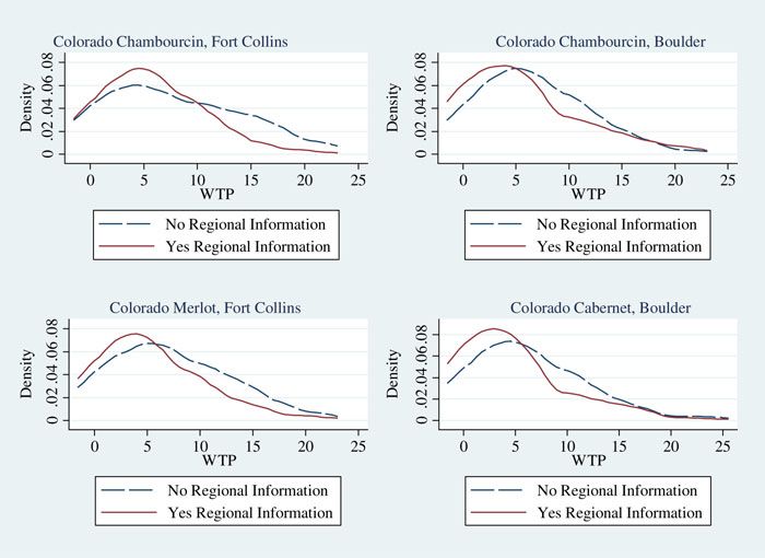
Figure 1 shows a Kernel density plot11 of the distribution of WTP with and
without the region of origin information. Observing the tails, it is evident that the
information treatment affected most prominently the right tail of the distribution,
where the potential Colorado wine customers reside.
11
To obtain the density, we discretized each WTP interval to its midpoint.https://doi.org/10.1017/jwe.2021.8
Downloaded from https://www.cambridge.org/core. Colorado State University Libraries, on 18 Apr 2021 at 22:58:47, subject to the Cambridge Core terms of use, available at https://www.cambridge.org/core/terms.
14 Consumer Stigma and the Reputation Trap Hypothesis
Figure 1
Kernel Density Estimates of High Frequency Wine Consumers’ WTP for Colorado Wines
with and without Regional Information
VI. Discussion and Policy Recommendations
We conducted an in-store test of the reputation trap hypothesis by measuring how
the region of origin information changes sensory perceptions and WTP for
Colorado wines. Our results are largely consistent with the presence of a stigma
against Colorado-produced wine, even though some findings require further investi-
gation. We found a statistically significant but rather small negative effect on taste
ratings (–0.11, on a 1–5 scale, p = 0.1), while the effect is larger for WTP ($–1.19,
p = 0.02). All results are robust to the inclusion of demographic controls such as
income and age. For the control California wines, we find no effect on taste, but
WTP unexpectedly decreased ($–1.05, p = 0.1) when we made regional information
available, a result deserving further discussion. Having found no evidence of a con-
founding effect attributable to income, and given that participants were much more
familiar with California than Colorado wines (see Table 3), our interpretation is that
the negative effect observed for California wines might be due to the generic nature
of the regional information we provided. The origin information in our experiments
did not indicate the specific American Viticultural Area (e.g., Napa Valley,
California), which consumers may expect to see with California wines. Typically,https://doi.org/10.1017/jwe.2021.8
Downloaded from https://www.cambridge.org/core. Colorado State University Libraries, on 18 Apr 2021 at 22:58:47, subject to the Cambridge Core terms of use, available at https://www.cambridge.org/core/terms.
Marco Costanigro and Becca B.R. Jablonski 15
California wines not reporting AVA are cheaper, large volume, bulk wines, mixing
grapes from multiple geographical areas. We speculate that this may have lowered
expectations about the market price of the wine, especially in a store environment.
Alternatively, participants may have displayed a home bias against California
wines. For example, Li, McCluskey, and Messer (2018) find differentiated effects
of information about water sourcing (conventional vs. recycled) on the WTP for
California vs. French wines.
There is little doubt that liquor stores proved to be a difficult environment for
Colorado wines. Very few participants in our experiment displayed a WTP above
typical market prices. Even more concerning, regional information affected
higher-WTP consumers the most, suggesting that the mass retail environment may
be poorly suited for promoting new wine regions. Price and quality competition in
retail stores is fierce, as the market is truly global. Consumers have access to world-
wide wines, from the ancient European regions of production (France, Italy, and
Spain) to rising New World stars (Australia, New Zealand, South Africa,
Argentina, and Chile). This puts some wine regions at a disadvantage, as price com-
petition is generally not feasible for small-scale producers, local messaging is ineffec-
tive (Loureiro, 2003), and stigma, as we found here, hinders quality perceptions.
That is not to say that nothing can be done. After all, California wines were often
snubbed before proving themselves in the famous 1976 “Judgement of Paris” tasting
competition (Taber, 2006). Of course, most novel U.S. wine regions are not endowed
with the favorable growing conditions of the California valleys. The key, it seems, is
to find a comparative advantage within a product niche, as Argentina did with
Malbec and New Zealand did with Sauvignon Blanc. This is a long-term proposi-
tion, but our results indicate that stigma is not aggravated when presenting unfamil-
iar varieties, so there is no downside to experimenting with new varietals.
Wineries in nontraditional wine regions could also actively engage in avoiding or
removing stigma. In the short term, a reasonable approach from a firm perspective is
to focus on quality, build brand recognition, and avoid stigma by pursuing a decou-
pling strategy (Slade Shantz et al., 2018). Based on regulations from the Alcohol and
Tobacco Tax and Trade Bureau (TTB),12 an appellation of origin can be the name of
a country, a state, a county, or an official American Viticultural Area, so there is no
binding obligation to display state identifiers on a label. Indeed, we observed that
several labels report the county or AVA information only, without mentioning
Colorado. This strategy is moot when retailers display wine by region of production,
but it may be useful when shelves are organized by variety.
Removing stigma is more complex. The literature distinguishes between core
stigma, caused by some evident and enduring core attribute, and event-based
stigma (Slade Shantz et al., 2018), which is linked to past performance. Stigma
12
27 CFR 4.25 see https://www.ttb.gov/appellations-of-origin.https://doi.org/10.1017/jwe.2021.8
Downloaded from https://www.cambridge.org/core. Colorado State University Libraries, on 18 Apr 2021 at 22:58:47, subject to the Cambridge Core terms of use, available at https://www.cambridge.org/core/terms.
16 Consumer Stigma and the Reputation Trap Hypothesis
affecting nontraditional wine regions is most likely event-based in nature, which is
easier to amend than core stigma. However, the market incentives motivating indi-
vidual wineries to engage in costly actions to amend stigma are weak. As regional
reputations are shared among all producers rather than owned by a single firm, indi-
vidual wineries can do little to change the current state of affairs (Winfree and
McCluskey, 2005). Costanigro, Bond, and McCluskey (2012) show that the presence
of an industry leader (i.e., an affirmed regional firm brand of larger size) can help
stimulate investment in collective reputation, but this is generally uncommon in
nascent wine regions.
State industry associations, when present, are perhaps best positioned to remove
stigma, but they have to strike a difficult balance. On the one hand, they are more
motivated than individual firms to take proactive measures and change public per-
ceptions. On the other, state-branded food marketing campaigns, similar to those
supporting local agricultural products (Nganje, Hughner, and Lee, 2011), run the
risk of being counterproductive in the presence of stigma. While we have no clear
prescription to offer, the recent Bud Light campaign provides a curious example
of creativity and what Slade Shantz et al. (2018) define as an “exploiting” strategy.
Facing a stigmatized product category (mass-produced lager beer, see Barlow,
Verhaal, and Hoskins (2018)), the brand embraced its common identity, poking
fun at the sophisticated craft beer drinker.
The winery and the tasting room remain the most favorable places to sell local
wine and counter stigma. In these environments, consumers are not just purchasing
wine but a product bundled with an experience, and per-bottle margins tend to be
higher (Barber, Donovan, and Dodd, 2008). Research has shown that the loca-
tion/environment in which experiences occur can improve quality perceptions and
WTP, and these effects are long-lasting (Pappalardo et al., 2019). Tourism activities,
however, tend to be seasonal, so the potential to increase volume is limited. The
easing of direct-to-consumer shipping laws13 provides an opportunity to follow
on-premises customers while bypassing liquor and grocery stores, but it requires
an adequate online presence and intentional marketing efforts to promote brand
loyalty.
VII. Limitations and Future Research
This study faced several limitations that should be considered when interpreting
results, but the limitations also suggest new avenues for research. For one, we con-
ducted the experiments in only two locations. This is common with experimental
approaches, but care should be taken in extrapolating our results. The anomalous
California result, and the hypothesis that state information without AVA lowers
13
According to the Wine Institute, only five U.S. states currently restrict direct-to-consumer shipping from
producing wineries. https://wineinstitute.compliancerules.org/state-map/https://doi.org/10.1017/jwe.2021.8
Downloaded from https://www.cambridge.org/core. Colorado State University Libraries, on 18 Apr 2021 at 22:58:47, subject to the Cambridge Core terms of use, available at https://www.cambridge.org/core/terms.
Marco Costanigro and Becca B.R. Jablonski 17
price expectations, should also be further investigated. This would require develop-
ing an experimental design including an AVA information treatment and its possible
interaction with the absence/presence of state information.
References
Andersen, S., Harrison, G. W., Lau, M. I., and Rutström, E. E. (2006). Elicitation using mul-
tiple price list formats. Experimental Economics, 9(4), 383–405. doi: 10.1007/s10683-006-
7055-6.
Barber, N. A., Donovan, J. R., and Dodd, T. H. (2008). Differences in tourism marketing
strategies between wineries based on size or location. Journal of Travel & Tourism
Marketing, 25(1), 43–57. doi: 10.1080/10548400802164889.
Barlow, M. A., Verhaal, J. C., and Hoskins, J. D. (2018). Guilty by association: Product-level
category stigma and audience expectations in the U.S. craft beer industry. Journal of
Management, 44(7), 2934–2960. doi: 10.1177/0149206316657593.
Beliveau, B. C., and Rouse, M. E. (2010). Prohibition and repeal: A short history of the wine
industry’s regulation in the United States. Journal of Wine Economics, 5(1), 53–68. doi:
10.1017/S1931436100001371.
Canziani, B., and Byrd, E. T. (2017). Exploring the influence of regional brand equity in an
emerging wine sector. Journal of Wine Economics, 12(4), 370–377. doi: 10.1017/
jwe.2017.30.
Carlsson, F., He, H., and Martinsson, P. (2013). Easy come, easy go: The role of windfall
money in lab and field experiments. Experimental Economics, 16(2), 190–207. doi:
10.1007/s10683-012-9326-8.
Castriota, S., and Delmastro, M. (2015). The economics of collective reputation: Evidence
from the wine industry. American Journal of Agricultural Economics, 97(2), 469–489.
doi: 10.1093/ajae/aau107.
Christenson, C., Martin, M., Thilmany McFadden, D., Sullins, M., and Jablonski, B. B. R.
(2016). 2016 Public Attitudes About Agriculture in Colorado [Unpublished Online
Report]. Colorado Department of Agriculture. Available from https://www.colorado.
gov/pacific/sites/default/files/2016%20Public%20Attitudes%20Report%20Final.pdf
Clark, J. K., and Jablonski, B. B. R. (2018). Federal policy, administration, and local food
coming of age. Choices, Quarter 3. Available from http://www.choicesmagazine.org/
choices-magazine/theme-articles/the-promise-expectations-and-remaining-questions-about-
local-foods/federal-policy-administration-and-local-food-coming-of-age.
Coate, S., and Loury, G. C. (1993). Will affirmative-action policies eliminate negative stereo-
types? American Economic Review, 83(5), 1220–1240.
Costanigro, M., Bond, C. A., and McCluskey, J. J. (2012). Reputation leaders, quality lag-
gards: Incentive structure in markets with both private and collective reputations.
Journal of Agricultural Economics, 63(2), 245–264. doi: 10.1111/j.1477-9552.2011.00331.x.
Edquist, G. (2014). Local Wineries Fight to Overcome Stigma, November 17. Available from
https://www.channel3000.com/madison-magazine/city-life/local-wineries-fight-to-overcome-
stigma/162785078.
Franken, J., Gómez, M., and Ross, R. B. (2018). Social capital and entrepreneurship in emerg-
ing wine regions. Journal of Wine Economics, 13(4), 419–428. doi: 10.1017/jwe.2018.37.
Gneezy, A. (2016). Field experimentation in marketing research. Journal of Marketing
Research, 54(1), 140–143. doi: 10.1509/jmr.16.0225.https://doi.org/10.1017/jwe.2021.8
Downloaded from https://www.cambridge.org/core. Colorado State University Libraries, on 18 Apr 2021 at 22:58:47, subject to the Cambridge Core terms of use, available at https://www.cambridge.org/core/terms.
18 Consumer Stigma and the Reputation Trap Hypothesis
Goffman, E. (1968). Stigma: Notes on the Management of Spoiled Identity. New York: Simon
and Schuster.
Hayes, D. J., Shogren, J. F., Shin, S. Y., and Kliebenstein, J. B. (1995). Valuing food safety in
experimental auction markets. American Journal of Agricultural Economics, 77(1), 40–53.
Kahneman, D., Knetsch, J. L., and Thaler, R. H. (1990). Experimental tests of the endowment
effect and the Coase theorem. Journal of Political Economy, 98(6), 1325–1348.
Lee, W. F., and Gartner, W. C. (2015). The effect of wine policy on the emerging cold-hardy
wine industry in the northern U.S. states. Wine Economics and Policy, 4(1), 35–44. doi:
10.1016/j.wep.2015.04.002.
Lee, W. F., Gartner, W. C., Song, H., Marlowe, B., Choi, J. W., and Jamiyansuren, B. (2018). Effect
of extrinsic cues on willingness to pay of wine: Evidence from Hong Kong blind tasting exper-
iment. British Food Journal, 120(11), 2582–2598. doi: 10.1108/BFJ-01-2017-0041.
Li, T., McCluskey, J. J., and Messer, K. D. (2018). Ignorance is bliss? Experimental evidence
on wine produced from grapes irrigated with recycled water. Ecological Economics, 153,
100–110. doi: 10.1016/j.ecolecon.2018.07.004.
Lockshin, L., Jarvis, W., d’Hauteville, F., and Perrouty, J.-P. (2006). Using simulations from
discrete choice experiments to measure consumer sensitivity to brand, region, price, and
awards in wine choice. Food Quality and Preference, 17(3–4), 166–178. doi: 10.1016/j.
foodqual.2005.03.009.
Loureiro, M. L. (2003). Rethinking new wines: Implications of local and environmentally
friendly labels. Food Policy, 28(5–6), 547–560. doi: 10.1016/j.foodpol.2003.10.004.
Mishina, Y., and Devers, C. E. (2012). On Being Bad: Why Stigma Is Not the Same as a Bad
Reputation. Oxford, UK: Oxford University Press. doi: 10.1093/oxfordhb/
9780199596706.013.0010.
Nelson, P. (1974). Advertising as information. Journal of Political Economy, 82(4), 729–754.
Nganje, W. E., Hughner, R. S., and Lee, N. E. (2011). State-branded programs and consumer
preference for locally grown produce. Agricultural and Resource Economics Review, 40(1),
20–32. doi: 10.1017/S1068280500004494.
O’Mahony, M., and Goldstein, L. R. (1986). Effectiveness of sensory difference tests:
Sequential sensitivity analysis for liquid food stimuli. Journal of Food Science, 51(6),
1550–1553. doi: 10.1111/j.1365-2621.1986.tb13857.x.
Pappalardo, G., Selvaggi, R., Pecorino, B., Lee, J. Y., and Nayga, R. M. (2019). Assessing
experiential augmentation of the environment in the valuation of wine: Evidence from
an economic experiment in Mt. Etna, Italy. Psychology & Marketing, 36(6), 642–654.
doi: 10.1002/mar.21202.
Plassmann, H., O’Doherty, J., Shiv, B., and Rangel, A. (2008). Marketing actions can mod-
ulate neural representations of experienced pleasantness. Proceedings of the National
Academy of Sciences, 105(3), 1050–1054. doi: 10.1073/pnas.0706929105.
Rickard, B. J., McCluskey, J. J., and Patterson, R. W. (2015). Reputation tapping. European
Review of Agricultural Economics, 42(4), 675–701. doi: 10.1093/erae/jbv003.
Shapiro, C. (1982). Consumer information, product quality, and seller reputation. Bell Journal
of Economics, 13(1), 20–35.
Slade Shantz, A., Fischer, E., Liu, A., and Lévesque, M. (2018). Spoils from the spoiled:
Strategies for entering stigmatized markets. Journal of Management Studies, 56(7),
1260–1286. doi: 10.1111/joms.12339.
Steenkamp, J.-B. E. M. (1990). Conceptual model of the quality perception process. Journal of
Business Research, 21(4), 309–333. doi: 10.1016/0148-2963(90)90019-A.
Taber, G. M. (2006). Judgment of Paris: California vs. France and the Historic 1976 Paris
Tasting That Revolutionized Wine. New York: Scribner.https://doi.org/10.1017/jwe.2021.8
Downloaded from https://www.cambridge.org/core. Colorado State University Libraries, on 18 Apr 2021 at 22:58:47, subject to the Cambridge Core terms of use, available at https://www.cambridge.org/core/terms.
Marco Costanigro and Becca B.R. Jablonski 19
TTBGov– Alcohol and Tobacco Tax and Trade Bureau (2019). American Viticultural Area
(AVA). Available from https://www.ttb.gov/wine/american-viticultural-area-ava.
Veale, R., and Quester, P. (2008). Consumer sensory evaluations of wine quality: The respec-
tive influence of price and country of origin. Journal of Wine Economics, 3(1), 10–29. doi:
10.1017/S1931436100000535.
Veale, R., and Quester, P. (2009). Do consumer expectations match experience? Predicting the
influence of price and country of origin on perceptions of product quality. International
Business Review, 18(2), 134–144. doi: 10.1016/j.ibusrev.2009.01.004.
Wansink, B., Payne, C. R., and North, J. (2007). Fine as North Dakota wine: Sensory expec-
tations and the intake of companion foods. Physiology & Behavior, 90(5), 712–716. doi:
10.1016/j.physbeh.2006.12.010.
WineAmerica.Org. (2014). United States Wine and Grape Industry. Available from https://
wineamerica.org/policy/by-the-numbers/.
Wines Vines Analytics (2019). Statistics. Available from https://winesvinesanalytics.com/statistics/
winery/.
Winfree, J. A., and McCluskey, J. J. (2005). Collective reputation and quality. American
Journal of Agricultural Economics, 87(1), 206–213.You can also read