Cavitation bubbles: a tracer for turbulent mixing in large rivers

River, Coastal and Estuarine Morphodynamics: RCEM2011
                                                                   © 2011 Tsinghua University Press, Beijing

Cavitation bubbles: a tracer for turbulent mixing in large rivers

Hugo CHAUVET, François METIVIER, Angela LIMARE
Equipe de dynamique des fluides géologiques
Institut de Physique du Globe de Paris, Sorbonne Paris Cité, Univ Paris Diderot
UMR 7154 CNRS, F-75005 Paris, France.

 ABSTRACT: On the Seine river in Paris, the high frequency of tourist boats traffic may exert a
significant impact on transport of sediments and thus on transport and residence time of pollutants. To
have a better understanding of anthropogenic effects and more generally to study rivers suspended
sediments dynamics, it is essential to quantify the river transport capacity. Turbulent mixing is one of
these transport mechanisms and we present here a simple technique to estimate lateral coefficient using
ADCP backscatter signal analysis. We realized several static measurements during low water discharge
(Q = 140 cubic meters per second) in which we can see a strong correlation between high backscatter
values and the passage of boats. We argue that these high backscatter values, in the center of Paris city,
are not due to a sediment plume but to cavitation bubbles. These high values suggest that resonant, ~10
micron bubbles are present in the flow in agreement with LISST grain size measurements. Given their
slow ascent velocity these particles can be used as passive markers to estimate the lateral turbulent mixing
coefficient. For this purpose we develop a dimensionless form of the sonar equation that, when coupled to
a simple lateral turbulent diffusion model, allows to compute lateral diffusion coefficients. These
estimates of lateral diffusion coefficient have an important implication for representative river water
sampling and can be very useful to calibrate numerical models of river flow and sediment transport.

1 INTRODUCTION

  The Seine river, in Paris city (Fig.1), is subject to effects of human activities like channel enlargement
and dam regulation of water level to allow navigation even during low water discharge period. This
navigation, especially the high frequency turnover of tourist boats disturbs the transport of sediments. In
order to study its impact on natural flow processes we develop a measurement protocol to study fluvial
dynamic along river cross-sections. Turbulent mixing plays an important role and estimation of the lateral
turbulent dispersion rate is essential to better understand sediment transport. Unfortunately these
estimations are still scarce because they involve deployment of measurement techniques such as dye
tracers (Fischer & Park, 1967), that are difficult to apply on large rivers. More recently Bouchez et al.
(Bouchez et al., 2010) used an isotopic method to estimate lateral turbulent mixing rate in Amazon river
using two tributaries with distinct chemical signatures. In this contribution we apply an original technique
to achieve this estimation using an Acoustic Doppler Current Profiler (ADCP).
  We here describe measurement setup and present results of granulometric and echo backscatter data
acquired in April 2010 in which we can infer the presence of bubbles. We then discuss echo backscatter
processing, in order to get a dimensionless concentration, and develop a simple 1D depth-averaged lateral
turbulent mixing model. Finally an application of this model is performed to estimate a coefficient of
lateral turbulent mixing.

2 FIELD MEASUREMENTS SETUP AND DATA

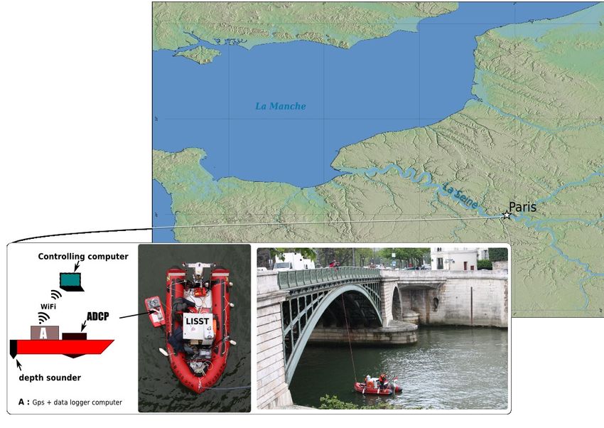
 To measure river currents and to study particle dynamics we setup an experimental device (Fig. 1)
composed of two main instruments: an ADCP (Rio Grande 1200 kHz from RD-Instrument) and a LISST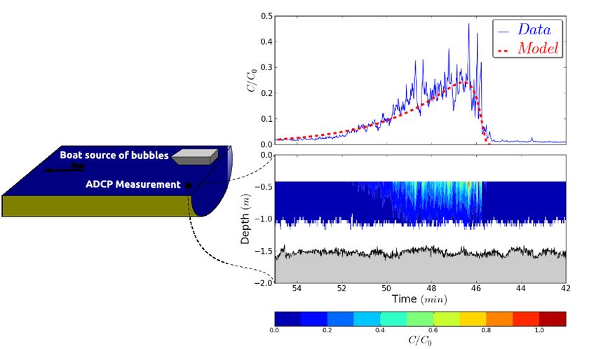

(Laser In Situ Scattering and Transmissometry, LISST-25 from Sequoia). We realised synchronous
measurements from a static location established using a rope from a bridge to stabilize an inflatable boat.
These measurements have been made at Sully bridge in the center of Paris city, where tourist boats pass
one by one and only in one way leading to more comprehensible backscatter signal.

                    Figure 1   Location of the present study and experimental devices setup

 ADCP instruments use the Doppler shift effect to calculate the velocity field and record the echo
backscatter over the entire water column within bin in the size range of 5 to 25 centimeter (Gordon, 1996).
This instrument is becoming widely used in rivers to estimate their discharges using moving-vessel
(Yorke & Oberg, 2002). Using it from a fixed location allow to record time series of velocity field (Muste
et al., 2004) and backscatter. The latter reflect the amount of sound reflectors (particles) present in the
insonified volume for each bins. It is generally used to estimate suspended solid concentration to study
sediment dynamic. This estimation is not straightforward and require independent concentration
measurements, like optical backscatter point sensor (OBS) (Gartner, 2004; Hoitink & Hoekstra, 2005) or
direct sample measurements (Holdaway et al., 1999), in order to calibrated echo backscatter. In this study
we use a LISST to complete backscatter measurements.
 The LISST is an optical instrument that calculates the concentration of particles for different particle
sizes using their light scattering properties (Agrawal & Pottsmith, 2000). It gives access to grain size
distribution for a given depth. The LISST-StreamSide measures particle sizes in 32 log-spaced size
classes in the size range of 1.25 to 250 microns. Both of these measurements are sensible to any kind of
reflectors like air bubbles or organic organisms so a particular attention has to be payed during
measurements in river especially if there is ship traffic.
 On backscatter time series recorded during this study, strong variations of backscatter are present (right
of Fig.2) and seems to be correlated with ship passages. This kind of backscatter shape can be due to
sediment plume or cavitation bubbles produced by ships propellers. Looking at particle size distribution
measured with the LISST during one of this high backscatter stage, presented on left of Fig.2, we can
remark the presence of 10 micron sized particles. For our ADCP transmitted sound pulses frequency
(1200 kHz), this size of particles corresponds to resonant radius for air bubbles (Brennen, 1995).
Furthermore concentrations measured with the LISST are small while backscatter variations are relatively
important, reflecting a greater sensitivity to presence of bubbles for the ADCP.

                                                     899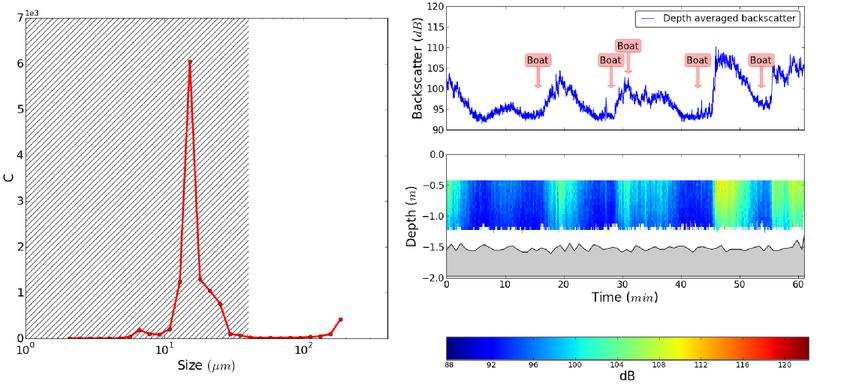

Figure 2 Left: Particle size distribution from LISST measurement, hashed zone represent bubble resonant radius
 for frequency of our ADCP (1200 kHz). Right: Backscatter time series recorded at Sully bridge, on bottom the raw
            ADCP backscatter with respect to time and depth and on top the depth-averaged backscatter

  Ship propellers are known to produce micron sized bubbles by cavitation present up to a depth of twice
the draft of ship (Miner, 1986). By looking at the shape of recorded backscatter signal with respect to
depth and time we can assume that particles have a slow ascending movement. Observations of ship’s
wake have been performed by Marmorino and Trump (Marmorino & Trump, 1996) who used an original
technique based on a 600 kHz ADCP in horizontal position and looking toward the ship’s wake. In their
measurements strong increases in backscatter values are cause by bubbles induced by ship propellers.
Finally looking at aerial pictures, we observe the presence of bubbles only inside Paris, whereas boats
outside the center of Paris produce bubbles and sediment plume (Fig.3). These observations put together
suggest that, in our measurements, we are in presence of bubbles.

Figure 3   Aerial images (from IGN) showing presence of sediment plume for a boat outside of Paris, on right, and a
                    tourist boat inside Paris producing only bubbles, on left. (© GEOPORTAIL)

 The backscatter record (right of Fig.2) is characterised by a rapid increase of his intensity just after boat
passages, then it slightly decrease up to a base level (~ 93 dB). This shape is characteristic of diffusive
processes and we can use this bubbles as a tracer to quantify lateral turbulent mixing coefficient.
Here, direct calibration, converting backscatter into concentrations, can not be performed because LISST
response to bubbles is not well correlated to backscatter variations. In order to use it to estimate the lateral
turbulent diffusion we use a dimensionless equation which allow to access to a concentration ratio.

3 BACKSCATTER PROCESSING

 Backscatter recorded by ADCP needs to be converted from ”counts” to decibel (dB) taking into account
geometrical effect of transducers and transmission loss due to water and sometimes particles (Gartner,

                                                       900

2004). The base of the theory is defined by a simplified form of the sonar equation (Urick, 1975) which
can be written as:
                                                                                                      (1)
where SL is the source level that can be computed from battery voltage only if a calibration have been
performed. RL is the reverberation level which relies echo intensity recorded by ADCP for each bins
in ”counts” to dB using RL=Kc RS, where RS is the relative signal strength and Kc is a conversion factor,
here taken to manufacturer value 0.45 dB/counts (Deines, 1999). The term 2TL is the two ways
transmission loss expressed like:

                                                                                                          (2)

with R the slant distance from transducer to bin, Ψ the near-field correction which is a function of R
(Downing et al., 1995) and αw the water absorption (Francois & Garrison, 1982). Finally the term TS of
equation 1 is the target strength linked to particle sound reflection properties and concentration (Thorne &
Hanes, 2002; Tessier, 2006):

                                                                                                          (3)

where C is mass concentration, σ, υs and ρs characterise the particle and V represent the ensonified
volume which is a function of R. Combining equation s 1,2 and 3, we can write (Tessier, 2006):

                                                                                                          (4)

 Usually this equation is calibrated with independent measurements of sediment concentration including
unknown terms in linear regression constants (Gartner, 2004).
 Here our independent concentration measurements with the LISST are insufficient or unusable with
bubbles to calibrate equation 4. Thus we consider the same kind of particles, bubbles, present overall the
water column. These bubbles produce the recorded backscatter allowing to define a reference level at a
given depth and, using equation 4, permit to define a reference concentration. Subtracting this reference
concentration to equation 4, we can write a dimensionless form of equation 4:

                                                                                                          (5)

in which subscribe 0 denote reference quantities. Equation 5 enables to avoid two unknown terms in
equation 4: one linked to particles response to an acoustic impulse and the other linked to the source level.
  To apply this backscatter processing, we first select a bubble cloud (typically between 45 and 55 minutes
in Fig.2). Then we find the maximum of backscatter to define the reference level. Finally we apply
transmission loss and ensonified volume corrections to obtain concentration ratio (equation 5).

4 LATERAL TURBULENT DIFFUSION MODEL

 River turbulent motions are known to have a diffusive behaviour. Along the lateral direction
(perpendicular to the mean flow) the approximation of a negligible mean lateral flow velocity component
can be done and thus turbulent diffusion can be written as (Rodi, 1993):

                                                                                                          (6)

where λ is the molecular diffusion which is assumed to be negligible and              is linked to the
concentration gradient along lateral direction (Taylor, 1953). Using these considerations the previous
equation leads to:

                                                                                                          (7)

where εy is the lateral turbulent diffusion constant which with a dimensional approach can be expressed as
εy=αu*H where u* is the bed shear velocity, H the river characteristic water depth and α the
dimensionless lateral mixing coefficient (Fischer & Park, 1967; Bouchez et al., 2010). This equation is
non-dimensioned, with C*=C/Ci, y*=y/w and t*=εy w-2t, to:
                                                    901

(8)

where Ci is the injected concentration and w the width of the the river.

5 RESULTS

 Equation 8 was numerically solved with concentration boundary conditions fixed to zero at each river
banks (i.e. C*=0 at y*=0 and y*=1). Assuming the localisation of the bubble source behind the ship
propeller, we use a concentration impulse at this position as an initial condition. To find the best lateral
turbulent diffusion coefficient, we first calculated the bed shear velocity by fitting the vertical velocity
profile recorded by the ADCP, using the law of the wall. Then we minimised the α parameter with the
depth-averaged concentration (Fig.4). We obtained α=17.1, equivalent to εy=1.8 m².s-1 with u*=0.07m.s-1
and H=1.5 m.

    Figuew 4      Result of lateral turbulent diffusion model against relative concentration from ADCP backscatter
 measured near Sully bridge. On the left: a cartoon representing the measurement situation. On the right: the bottom
part of the plot shows the relative concentration with respect to depth and time while the upper part is depth-averaged
                      backscatter (in blue) and the result of the turbulent diffusion model (in red)

  This simple model gives reasonable results and reproduces well the shape of concentration signal. The
resulting value of lateral mixing coefficient is similar to the one found by Bouchez et al. (Bouchez et al.,
2010) on the Amazon river: εy=1.8 m².s-1, with u*=0.05 m.s-1 and H=25m. In literature the dimensionless
transverse mixing coefficient, α, varies over a large range from 0.1 to 3.5 (Rutherford, 1994). Compared
to these values, the Seine transverse mixing coefficient is very high and may reflect effects of ship
propellers rotation on mixing efficiency.

6 CONCLUSION

 For the Seine river, in Paris city, ADCP and LISST measurements show essentially the presence of
bubbles produced by ship’s propellers. Their effects in recorded signals have to be taken into account in
order to realise a fair estimation of sediments concentration with these instruments. Nevertheless, bubbles
can be successfully used to estimate lateral turbulent mixing coefficient in this river. Here, this estimation
leads to a high value of lateral mixing coefficient. Using a distance criterion, based on lateral turbulent
                                                         902

mixing coefficient, we can infer an homogenisation distance (Bouchez et al., 2010):

                                                                                                                (9)

 During law discharge period, the Seine typical mean velocity is around 0.3 m.s-1 and his typical width is
around 100 m. With εy=1.8 m².s-1, equation 9 gives an homogenisation distance of 2 Km. With this value,
we argue that high frequency turnover of tourist boats may prevent sediments deposition during low water
discharge period. Measurements of sediment concentration and sediment plume produced by boats
outside of Paris city can help to constrain this hypothesis. Furthermore, other measurements using
bubbles signal recorded by ADCP are required to constrain lateral turbulent mixing coefficient in the
Seine river and ascertain the influence of boats turnover on the mixing coefficient.

7 ACKNOWLEDGEMENT

 The research program was funded by Mairie de Paris, Paris 2030 Research program (Convention
DASCO/2008-175). This is IPGP contribution 3167.

REFERENCES

Agrawal, Y., & Pottsmith, H. (2000). Instruments for particle size and settling velocity observations in sediment
    transport. Marine Geology, 168(1-4), 89–114.
Bouchez, J., Lajeunesse, E., Gaillardet, J., France-Lanord, C., Dutra-Maia, P., & Maurice, L. (2010, February).
    Turbulent mixing in the Amazon River: The isotopic memory of confluences. Earth and Planetary Science
    Letters, 290(1-2), 37–43.
Brennen, C. (1995). Cavitation and bubble dynamics. Oxford University Press, USA.
Deines, K. (1999). Backscatter estimation using broadband acoustic Doppler current profilers. In Current
    measurement, 1999. proceedings of the ieee sixth working conference on (pp. 249–253).
Downing, A., Thorne, P., & Vincent, C. (1995). Backscattering from a suspension in the near field of a piston
    transducer. The Journal of the Acoustical Society of America, 97, 1614.
Fischer, H., & Park, M. (1967). Transverse mixing in a sand-bed channel. US Geological Survey. Professional
    paper.
Francois, R., & Garrison, G. (1982). Sound absorption based on ocean measurements. Part II: Boric acid contribution
    and equation for total absorption. The Journal of the Acoustical Society of America, 72, 1879.
Gartner, J. (2004). Estimating suspended solids concentrations from backscatter intensity measured by acoustic
    Doppler current profiler in San Francisco Bay, California. Marine geology, 211(3-4), 169–187.
Gordon, R. L. (1996). Accoustic Doppler Current Profiler Principles of Operation a Practical Primer. RD Instruments,
    San Diego.
Hoitink, A., & Hoekstra, P. (2005). Observations of suspended sediment from ADCP and OBS measurements in a
    mud-dominated environment. Coastal engineering, 52(2), 103–118.
Holdaway, G., Thorne, P., Flatt, D., Jones, S., & Prandle, D. (1999). Comparison between ADCP and transmissometer
    measurements of suspended sediment concentration. Continental shelf research, 19(3), 421.
Marmorino, G., & Trump, C. (1996). Preliminary Side-Scan ADCP Measurements across a Ship’s Wake. Journal of
    Atmospheric and Oceanic Technology, 13, 507.
Miner, E. (1986). Near-surface bubble motions in sea water (Tech. Rep.). Naval Research Lab Washington DC.
Muste, M., Yu, K., Pratt, T., & Abraham, D. (2004). Practical aspects of ADCP data use for quantification of mean
    river flow characteristics; Part II: fixed-vessel measurements. Flow measurement and instrumentation, 15(1), 17-
    28.
Rodi, W. (1993). Turbulence models and their application in hydraulics: a state-of-the art review. Aa Balkema.
Rutherford, J. (1994). River mixing. Wiley & Sons.
Taylor, G. (1953). Dispersion of soluble matter in solvent flowing slowly through a tube. Proceedings of the Royal
    Society of London. Series A. Mathematical and Physical Sciences, 219(1137), 186.
Tessier, C. (2006). Caractérisation et dynamique des turbidités en zone côtières: l’exemple de la région maritime
    bretagne sud. Unpublished doctoral dissertation, UniversitéBordeaux 1.
Thorne, P., & Hanes, D. (2002). A review of acoustic measurement of small-scale sediment processes. Continental
    Shelf Research, 22(4), 603–632.
Urick, R. (1975). Principles of Underwater Sound, (2nd ed.). McGraw Hill, New York.
Yorke, T., & Oberg, K. (2002). Measuring river velocity and discharge with acoustic Doppler profilers. Flow
    Measurement and Instrumentation, 13(5-6), 191-195.

                                                        903