CHARACTERIZING THE SPATIAL DISTRIBUTION OF GIANT PANDAS IN CHINA USING MULTITEMPORAL MODIS DATA AND LANDSCAPE METRICS
←
→
Page content transcription
If your browser does not render page correctly, please read the page content below
CHARACTERIZING THE SPATIAL DISTRIBUTION OF GIANT PANDAS IN CHINA
       USING MULTITEMPORAL MODIS DATA AND LANDSCAPE METRICS

                                     X.P. Ye a, b, *, T.J. Wang a, A.K. Skidmore a, A.G. Toxopeus a
  a
      ITC, Natural Resources Department, Hengelosestraat 99, 7500AA Enschede, The Netherlands – (ye17188, tiejun,
                                               skidmore, toxopeus)@itc.nl
       b
         Foping National Nature Reserve, No. 89 Huangjiawan Road, Foping, 723400 China – pandayxp@gmail.com

                                                     Commission VIII, WG VIII/11

KEY WORDS: Multitemporal, Forest, Landscape, Spatial, Configuration, Modelling, Knowledge Base

ABSTRACT:

Although forest fragmentation and degradation have been recognized as one of major threats to wild panda population, little is
known about the relationship between panda distribution and forest fragmentation. This study is unique as it presents a first attempt
at understanding the effects of forest fragmentation on panda spatial distribution for the entire wild panda population. Using a
moving window with a radius of 3 km, landscape metrics were calculated for two classes of forest (i.e. dense forest and sparse forest)
which derived from a complete year of MODIS 250 m EVI multitemporal data in 2001. Eight fragmentation metrics that had highest
loadings in factor analyses were selected to quantify the spatial heterogeneity of forests. It was found that the eight selected metrics
were significantly different (P < 0.05) between panda presence and absence. The relationship between panda distribution and forest
heterogeneity was explored using forward stepwise logistic regression. Giant pandas appear sensitive to patch size and isolation
effects associated with forest fragmentation. The R2 value (0.45) of the final regression model indicates that landscape metrics partly
explain the distribution of giant pandas, though a knowledge-based control for elevation and slope improved the explanation to
74.9%. Findings of this study imply that the design of effective conservation area for wild panda must include large, contiguous and
adjacent forest areas.

                     1. INTRODUCTION                                   landscape elements are species-specific (Cain et al., 1997;
                                                                       Saura, 2004), appropriate land cover classes and spatial
The giant panda (Ailuropoda melanoleuca) is one of the world’s         resolution are critical to link response variables of species
most endangered mammals. Fossil evidence suggests the giant            (Taylor et al., 1993; Hamazaki, 1996; Corsi et al., 2000) with
panda were widely distributed in warm temperate or subtropical         landscape metrics (Turner et al., 1989; Frohn, 1998; Wu et al.,
forests over much of eastern and southern China (Schaller,             2000). Time-series of 16-day composite MODIS 250 m
1994). Today this range is restricted to temperate montane             Enhanced Vegetation Index (EVI) product, with a broad
forests across five separate mountain regions, where bamboo is         geographical coverage (swath width 2 330 km), intermediate
the dominant understory forest plant (Schaller, 1994; Hu, 2001).       spatial resolution and high temporal resolution, offers a new
According to the Third National Panda Survey (State Forestry           option for large area land cover classification (Bagan et al.,
Administration of China, 2006), the number of giant panda              2005; Liu and Kafatos, 2005). EVI is designed to minimize the
individuals increased in the last decades, but their distribution is   effects of the atmosphere and soil background (Huete et al.,
discontinuous, with 24 isolated populations.                           2002), and was found to be responsive to canopy structure (Gao
                                                                       et al., 2000).
Forest fragmentation and degradation have already been
recognized as major threats that pose a great danger for panda         The primary aim of this paper was to understand how the entire
population (Schaller, 1994; Hu, 1997; Hu, 2001). However,              giant panda population relates to forest fragmentation. Specific
little is known about the distribution pattern of giant pandas at a    research questions included: (1) Which landscape metrics
national scale, as previous studies focused on the local               characterize fragmentation of forests occupied by giant pandas?
relationships of panda occurrences and micro-environmental             (2) What are the relationships between the distribution of giant
factors (Hu, 2001; Lindburg and Baragona, 2004). In other              pandas and forests fragmentation? (3) Do landscape metrics
words, to date no quantitative and systematic studies have             explain what proportion of the distribution of the giant panda?
attempted to address the panda distribution with relation to
fragmentation of forested landscapes (e.g. forest patch size,
patch isolation and aggregation), especially over the entire                       2. MATERIALS AND METHODS
range of wild giant pandas.
                                                                       2.1 Study Area
A large number of landscape metrics have been proposed to
quantify landscape patterns based on land cover as derived from        The study area (Figure 1) incorporates the 45 administrative
remotely sensed data (Hulshoff, 1995; Gustafson, 1998).                counties in Shaanxi, Gansu, and Sichuan provinces of China
Because most landscape metrics are scale-dependent and                 which cover the entire giant panda distribution area, and

* Corresponding author.

                                                                   1039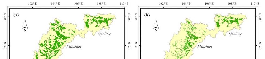
The International Archives of the Photogrammetry, Remote Sensing and Spatial Information Sciences. Vol. XXXVII. Part B8. Beijing 2008

sampled during the Third National Panda Survey (State                geometrically reprojected to form a mosaic with a pixel size of
Forestry Administration of China, 2006). The total area is about     250 m for reference data extraction. The DEM was clipped
160 000 km2, with the elevation ranging from 560 m to 6 500 m.       from the Shuttle Radar Topography Mission (SRTM) 90 m
The study area cross five mountain regions along the eastern         seamless digital topographic data and resampled to 250 m using
edge of the Tibetan Plateau: Qinling, Minshan, Qionglai,             a nearest neighbour operator. The Bio-Climatic Division Map
Xiangling, and Liangshan. Qinling region is the northernmost         of China (Liu et al., 2003) was rasterized with a pixel size of
area of the present-day distribution of the giant panda (Hu,         250 m to improve land-cover classification. All data were
2001), in which covered with deciduous broadleaf and                 geometrically rectified and geo-referenced to ensure proper
subalpine coniferous forests (Ren, 1998). Minshan and Qionglai       mutual registration and geographic positioning.
regions, with steep terrain, cool and humid climate, are the
biggest distribution area of the giant panda (Hu, 2001), in which    2.2.2 Land-cover Characterization: Land-cover map for
dense coniferous forests with an understory of bamboo thrive in      the study area was derived from retained five PCs in ENVI 4.3
the middle and upper elevations (China Vegetation Compiling          (ITT Industries, Inc). Because the giant panda has a strong
Committee, 1980). Xiangling and Liangshan regions are                preference for high forest canopy cover (Hu et al., 1985; Hu,
southernmost panda distribution area, covered by evergreen           2001), we used five categories based on the NLCD-2000 land-
broadleaf forests and coniferous forests (China Vegetation           cover classification system (Liu et al., 2002) to represent the
Compiling Committee, 1980).                                          land-cover. Using a combination of unsupervised and
                                                                     supervised methods and integrated with the DEM and bio-
                                                                     climatic division data, land covers were classified as dense
                                                                     forest (canopy cover > 30%), sparse forest (canopy cover <
                                                                     30%), grassland, cropland, and nonvegetated. The resulting land
                                                                     cover map with a grain size of 250 m and an overall accuracy of
                                                                     84% (kappa 0.8) was used for landscape metrics computation.

                                                                     2.2.3 Panda Presence-Absence Data: Because panda
                                                                     occurrence data were collected by an exhaustive survey
                                                                     throughout the study area (State Forestry Administration of
                                                                     China, 2006), any panda occurrence-free location can be
                                                                     potentially considered as a true absence. By buffering the
                                                                     occurrence points, it becomes possible to generate randomly
                                                                     distributed pseudo-absences and ameliorate the set towards true
                                                                     absences (Olivier and Wotherspoon, 2006). Initially 3 000
                                                                     random points were sampled within the forested areas with the
                                                                     minimum distance of 3 km between each other and minimum
                                                                     distance of 3 km to forest edges. Similar to the method of
                                                                     Olivier and Wotherspoon (2006), points were overlapped with a
                                                                     3-km buffer of panda occurrence points, 1 124 points that
                                                                     completely lay within the buffer zone were selected as panda
                                                                     presence samples, and 1 278 points that (1) located outside the
 Figure 1. Map of the study area delineated in red polygon. The      buffer zone and (2) at a minimum distance of 3 km to the
image presented is MODIS 250m EVI 16-day composite during            boundary of the buffer zone were selected as panda absence
                  Julian day 193-209 of 2001.                        samples. In light of the giant panda biology (Hu, 2001), samples
                                                                     located in the areas above 3 500 m or with a slope greater than
2.2 Environmental and Species Data                                   50º were discarded. The Moran’s I statistic (Moran’s I = 0.03, Z
                                                                     = 1.91, P > 0.05) indicated that the spatial autocorrelation was
2.2.1 Remote Sensing Data Preparation: MODIS 250 m                   insignificant in the samples (Upton and Fingleton, 1985).
EVI time-series were downloaded and extracted by tile,
mosaicked, reprojected from the Sinusoidal to the Albers Equal       2.3 Selection of Landscape Metrics for Quantifying Forest
Area Conic projection using a nearest neighbour operator, and        Fragmentation
subset to the study area. To diminish the noise mainly caused
by remnants of clouds, a clean, smooth time-series of EVI were       Initially 26 landscape metrics (Table 1) were computed from
reconstructed from raw EVI time-series by employing an               the land cover map with a constant spatial extent for the two
adaptive Savitzky–Golay smoothing filter in TIMESAT                  forest classes in FRAGSTATS 3.3 (McGarigal and Marks,
package (Jönsson and Eklundh, 2004). The resulting smoothed          1995). A moving window radius for computation was set to 3
time-series for 2001 (23 dimensions) were transformed into           km, so as to have a landscape extent equivalent to the territory
principal components (PCs) using a Principal Component               of an adult giant panda (Hu, 2001; Pan, 2001). After
Analysis (Byrne et al., 1980; Richards, 1984) to reduce data         computation, values of metrics were extracted to panda
volume, and the first five PCs (accounting for 99.1% of              presence-absence points by an extraction tool in Spatial Analyst
variance in smoothed EVI time-series) were retained for further      Tools of AcrGIS 9.2 (ESRI Inc. 2007).
analysis.
                                                                     To obtain a set of redundancy-free metrics for quantifying the
Ancillary data that were used in this study included the             spatial configurations of forest, firstly a partial correlation
National Land Cover Map of China (NLCD-2000), a digital              analysis with controlling for the effect of elevation was
elevation model (DEM), and the Bio-Climatic Division Map of          employed to eliminate highly correlated metrics. Of the pairs of
China. The NLCD-2000 Map, which developed from hundreds              metrics with correlation coefficients ≥ |0.9|, only one metric was
of TM and ETM images in 2000 (Liu et al., 2002), was                 retained based on the criteria: (1) metrics that commonly used

                                                                  1040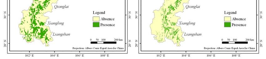
The International Archives of the Photogrammetry, Remote Sensing and Spatial Information Sciences. Vol. XXXVII. Part B8. Beijing 2008

in literatures; (2) density metrics and distribution statistics      construct a model with good fit to the data, in which the
metrics were preferred to absolute metrics (Riitters et al., 1995;   variable with the most significant change in deviance at each
Griffith et al., 2000). With the remaining metrics, a factor         stage was incorporated into the model until no other variables
analysis (Riitters et al., 1995; Cain et al., 1997) was performed,   were significant at the P < 0.05. The best model was selected
and non-correlated factors were extracted using a principal          based on Nagelkerke R2 and Hosmer-Lemeshow goodness of fit
components method with orthogonal rotations and retained by          test (Hosmer and Lemeshow, 2000; Davis, 2002). The panda
the Kaiser rule that factor’s eigenvalue > 1 (Bulmer, 1967). The     presence-absence samples were randomly split into two parts,
metrics with highest absolute loading on each of retained            one for model building (n = 2 000), another for model
factors were selected as landscape variables. By this process,       evaluation (n = 402). All statistical analyses were conducted in
the multicollinearity in metrics was no longer problematic           SPSS 15.0 (SPSS Inc. 2006).
(Variance-Inflation Factors < 5 and tolerance > 0.2 (Sokal and
Rohlf, 1994)).                                                       2.4.3 Spatial Implementation of Model: Because the
                                                                     logistic regression model was built only on landscape metrics,
                                                                     whereas the distribution of the giant panda was limited by a
   Acronym             Metric name                                   range of environmental conditions such as terrain features, the
   LPI                 Largest Patch Index                           model may overestimate panda distribution regardless of
   LSI                 Landscape Shape Index                         environmental tolerances and preferences of the giant panda.
   PD                  Patch Density                                 Hence, a knowledge-based control was applied by integrating
   PLAND               Percentage of Landscape                       the logistic regression model with elevation and slope to
   ED                  Edge Density                                  mitigate the risk of over-prediction, described as below:
   AREA                Mean Patch Area
   GYRATE              Radius of Gyration Distribution
   CONTIG              Contiguity Index                                                    P '= P ×C
                                                                                             i     i   ele
                                                                                                             × C slope              (1)
   FRAC                Fractal Dimension Index
   PARA                Perimeter Area Ratio
   SHAPE               Shape Index                                   where    Pi′ = refined probability
   CPLAND              Core Percentage of Landscape                           Pi = probability estimated by logistic regression model
   DCAD                Disjunct Core Area Density                             Cele = conditional probability related to elevation
   DCORE               Disjunct Core Area Distribution                        Cslope = conditional probability related to slope
   CAI                 Core Area Index
   CORE                Core Area                                     The knowledge-based rules for control were formulated based
   COHESION            Patch Cohesion Index                          on the integration of knowledge from several sources: (1)
   CONNECT             Connectance Index                             literatures (Hu, 2001; Pan, 2001); (2) detailed discussion with
   ENN                 Euclidian Nearest Neighbour Index             several specialists; (3) knowledge acquired from field
   PROX                Proximity Index                               observations. Spatial implementations of the logistic regression
   AI                  Aggregation Index                             model and knowledge-based control were achieved in ERDAS
   CLUMPY              Clumpy Index                                  IMAGINE 9.1 (LLC, 2006).
   DIVISION            Landscape Division Index
   IJI                 Interspersion Juxtaposition Index             2.4.4 Model Evaluation: The performance of final logistic
   PLADJ               Percentage of Like Adjacencies                regression model was assessed by overall accuracy, sensitivity
   SPLIT               Splitting Index                               and specificity, kappa coefficient and Z-test using an
                                                                     independent panda presence-absence data (n = 402). Sensitivity
Table 1. Landscape metrics used in this study. All metrics were      is defined as the proportion of correctly predicted presence to
     computed for dense forest and sparse forest. Detailed           the total number of presence in testing samples; and specificity
      descriptions refer to McGarigal and Marks (1995).              is the proportion of correctly predicted absence to the total
                                                                     number of absence in testing samples (Fielding and Bell, 1997).
2.4 Characterizing the Panda Distribution with Metrics               The kappa coefficient and its variance (Cohen, 1960; Congalton,
                                                                     1991; Skidmore et al., 1996) were computed and the effect of
2.4.1 Significance Testing: Representative metrics were              the knowledge-based control was examined through a Z-statistic
compared between forest areas with panda presences and               using kappa coefficients (Cohen, 1960; Congalton, 1991). A
absences. Because some metrics did not meet the assumption of        threshold of 0.5 was arbitrarily selected to convert the
homogeneity of variances and some were non-normally                  continuous probability surface to a discrete panda presence-
distributed, a Brown-Forsythe's F test (Rutherford, 2001) and        absence map. A probability greater than or equal to 0.5 was
nonparametric Mann-Whitney U test were employed to test              coded as presence, and less than 0.5 was absence. However, this
whether metrics are significantly different between panda            value may not be optimal in all cases (Manel et al., 1999).
presences and absences. Metrics with significant difference          Hence, a sensitivity analysis was conducted to consider
were used for further model building. All tests were conducted       thresholds from 0.3 to 0.7.
in SPSS 15.0 (SPSS Inc. 2006).

2.4.2 Logistic Regression Analysis: The binomial logistic                                        3. RESULTS
regression, a common statistical method used to estimate
occurrence probabilities in relation to environmental predictors     3.1 Representative Metrics for Forest Fragmentation
(Cowley et al., 2000), was employed for delineating the relation     Quantification
between panda presence-absence and representative metrics.
                                                                     From the factor analyses, eight metrics were selected as
Stepwise model-fitting with forward selection was used to help
                                                                     representative metrics for quantifying forest fragmentation, four

                                                                  1041
The International Archives of the Photogrammetry, Remote Sensing and Spatial Information Sciences. Vol. XXXVII. Part B8. Beijing 2008
metrics measure dense forest and four metrics measure sparse absences (Table 2), indicating these metrics are important
forest (Table 2). In general, these eight metrics measure three factors for the distribution of giant pandas. Patches of forest
aspects of the forests: patch area/edge, patch connectivity, and occupied by giant pandas tended to be larger, closer together
patch aggregation. and more contiguous. All metrics were used for logistic
Statistical tests show that all eight representative metrics were regression model building.
significantly different (P < 0.05) between panda presences and
Presence (n=1124) Absence (n=1278) Brown-Forsythe's Mann-Whitney
Metrics
Mean ± S.D. Mean ± S.D. F test U test
ED of dense forest 22.6 ± 5.6 16.8 ± 7.2 507.0 (P < 0.01) -20.2 (P < 0.01)
LPI of dense forest 53.4 ± 21.8 33.7 ± 25.4 416.3 (P < 0.01) -19.1 (P < 0.01)
PROX of dense forest 16.1 ± 10.9 9.9 ± 9.4 218.0 (P < 0.01) -12.8 (P < 0.01)
CLUMPY of dense forest 0.4 ± 0.1 0.4 ± 0.3 62.1 (P < 0.01) -14.5 (P < 0.01)
AREA of sparse forest 75.9 ± 124.1 184.3 ± 280.3 156.3 (P < 0.01) -14.4 (P < 0.01)
LSI of sparse forest 4.0 ± 0.8 3.7 ± 0.8 97.9 (P < 0.01) -10.3 (P < 0.01)
PROX of sparse forest 6.1 ± 6.3 9.46 ± 8.6 121.5 (P < 0.01) -8.8 (P < 0.05)
CLUMPY of sparse forest 0.4 ± 0.2 0.4 ± 0.2 89.3 (P < 0.01) -13.1 (P < 0.01)
Table 2. Summary statistics and results of Brown-Forsythe's F test and Mann-Whitney U test for eight representative metrics
between panda presence and absence.
3.2 The Logistic Regression Model 3.3 Model Performance
Of eight representative metrics, four metrics were significant at The logistic regression model explains around 45% of the
P < 0.01 (Table 3) and the rest were not included into the final overall variance of the metrics in training dataset (R2 = 0.45).
model (at P < 0.05), indicating that patch size, edge density, However, the Hosmer-Lemeshow statistic was 15.864 (df = 8, P
and clumpiness of dense forest play significant roles in defining = 0.04), pointing out that the model might not fit the data
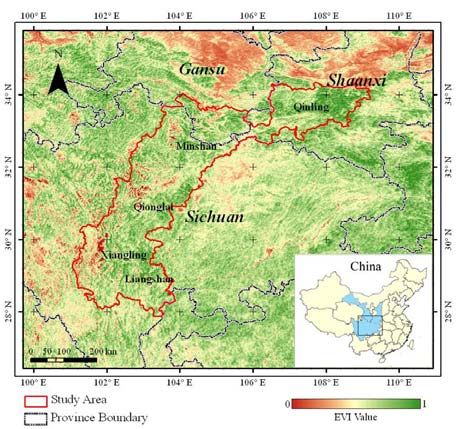
panda distribution. adequately. By applying the knowledge-based control to the
model, the overall accuracy and specificity increased around
5% and 13% respectively (Table 4), and predicted panda
Parameter Coefficient S.E. P presence shrank mainly in Qionglai, Xiangling, and Liangshan
ED of dense forest 0.160 0.010 < 0.001 (Figure 2). The Z-test for kappa coefficients shows that the
LPI of dense forest 0.042 0.003 < 0.001 accuracy of the mapping was significantly improved by
CLUMPY of dense forest -1.475 0.335 < 0.001 applying the knowledge-based control (P < 0.05). The
AREA of sparse forest 0.001 0.000 < 0.01 sensitivity analysis indicated that the threshold of 0.5 is
Constant -4.736 0.363 < 0.001 appropriate for transforming continuous probabilities of panda
occurrence to discrete panda presence-absence, where the
Table 3. Parameter estimates of the final logistic regression sensitivity-specificity difference (Liu et al., 2005) reaches the
model. minimum.
Figure 2. Presence-absence of the giant panda predicted by the logistic regression model (threshold = 0.5): (a) without knowledge-
based control; (b) with knowledge-based control for elevation and slope.
1042The International Archives of the Photogrammetry, Remote Sensing and Spatial Information Sciences. Vol. XXXVII. Part B8. Beijing 2008
network, are also necessary since they have direct or indirect
Modelling influences on giant pandas.
Without control With control
Overall accuracy 69.9% 74.9% The random panda presence-absence data may also affect the
accuracy of prediction, mainly because the data were inferred
Sensitivity 79.5% 77.6%
based on panda occurrences records instead of ground truth.
Specificity 58.5% 71.6% Exhaustive searches should be conducted in limited areas in
Kappa 0.39 0.49 order to provide accurate data on absences as they refine the
Kappa variance 0.00048 0.00044 model, as suggested by Brotons et al. (2004). In addition, the
Z 3.42 (P < 0.05) heterogeneity in forests across the panda distribution area can
also increase within-group variance in the training samples, and
Table 4. Statistics for evaluation of model performance. consequently decrease the power of the model. This may be
mitigated by dividing the study area into several homogeneous
forested landscapes.
4. DISCUSSION
Furthermore, landscape metrics may be sensitive to the level of
4.1 Distribution of giant pandas in relation to forest detail in categorical map data that is determined by the schemes
fragmentation used for map classification (Turner et al., 2001). In this study,
forests were categorized into dense forest (canopy cover > 30%)
From an ecological point of view, every species has its and sparse forest (canopy cover < 30%). The division is
particular position in the ecosystem, which is termed ‘niche’ practical as it was used in UNEP-WCMC's forest classification
(Elton, 2001). The giant panda is a forest inhabitant with (http://www.unep-wcmc.org/forest/fp_background.htm). It is
exclusive territory, thus the spatial pattern and forest patch also ecologically meaningful because giant pandas have been
plays an important role in the distribution of the giant panda. In proven that have a strong preference for forest patches with a
this study, both the Brown-Forsythe's F test and nonparametric high canopy cover (Hu, 2001). The test for the sensitivity of
Mann-Whitney U test showed that eight representative metrics landscape metrics towards different division of forests may help
were significantly different between panda presence and the understanding of the relationship between forest spatial
absence, indicating the heterogeneity of forest has a significant patterns and the response of the giant panda; but this is beyond
contribution to the distribution of giant pandas. Of the four the objective of this study.
metrics included in the logistic regression model, three metrics
measure patch area/edge, pointing out that the giant panda
appear sensitive to patch size and isolation effects associated 5. CONCLUSION
with forest fragmentation. The giant panda tends to occur in
larger, more contiguous (or less fragmented), but less This study demonstrated a successful approach for modelling
aggregated dense forest patches. A larger dense forest patch or the spatial distribution of giant pandas from multitemporal
contiguous patches can potentially provide good conditions of MODIS 250 m EVI data and landscape metrics. Eight metrics
food and shelter because of the high patch connectivity. The were selected to quantify forest fragmentation. All metrics were
preference of less aggregated forest patches may relate to panda significantly different between the forest patches with panda
migration or dispersal, because high aggregated patches will presences and absences. Forest patch size, edge density, and
increase the cost of migration or dispersal, e.g. high risk of patch aggregation were found play more significant roles in
being preyed, lack of shelter. panda distribution. Selected landscape metrics partly explained
the distribution of giant pandas, though a knowledge-based
4.2 Model performance and its factors control for elevation and slope improved the explanation
significantly. Findings of this study have profound implications
As demonstrated in this study, logistic regression model with for wild giant panda conservation.
knowledge-based control for the effect of elevation and slope is
capable of predicting the spatial distribution of the giant panda
using landscape metrics. Logistic regression itself is a REFERENCES
transformed linear regression which merely depends on
explanatory variables included in the model, whereas the Bagan, H., et al., 2005. Land cover classification from modis
distribution of the giant panda is also limited by other physical evi times-series data using som neural network. International
conditions of environment. The absence of those factors may Journal of Remote Sensing 26(22): 4999 - 5012.
result in the bias in modelling. This problem can be diminished
by applying an appropriate knowledge-based control, However, Brotons, L., et al., 2004. Presence-absence versus presence-only
to design an ecologically meaningful control needs adequate modelling methods for predicting bird habitat suitability.
relevant knowledge and well-understanding of the relationship Ecography( 27): 437-448.
between the species and the environmental factors.
Bulmer, M. G., 1967. Principles of statistics. Dover, New York,
A fundamental assumption of this study is that bamboo is 252.
sufficient and thus not a constraint of panda distribution. In fact,
Byrne, G. F., et al., 1980. Monitoring land-cover change by
bamboo resources are unevenly distributed across five mountain
principal component analysis of multitemporal landsat data.
regions (State Forestry Administration of China, 2006). To
Remote Sensing of Environment 10: 175-184.
accurately map the distribution of giant pandas or design
corridors, spatial pattern and quality information of bamboo Cain, D. H., et al., 1997. A multi-scale analysis of landscape
forests is required. In addition to bamboo information, other statistics. Landscape Ecology 12(4): 199-212.
environmental factors, such as forest compositions and road
1043The International Archives of the Photogrammetry, Remote Sensing and Spatial Information Sciences. Vol. XXXVII. Part B8. Beijing 2008
China Vegetation Compiling Committee, C., 1980. China Jönsson, P. and L. Eklundh, 2004. Timesat - a program for
vegetation. Science Press, Beijing. analyzing time-series of satellite sensor dat. Computers and
Geosciences 30: 833–845.
Cohen, J., 1960. A coefficient of agreement for nominal scales.
Edu. Psychol. Measure 20: 37-46. Lindburg, D. e. and K. e. Baragona, 2004. Giant panda's :
Biology and conservation. University of California Press,
Congalton, R. G., 1991. A review of assessing the accuracy of Berkeley etc., 308.
classifications of remotely sensed data. Remote Sensing of
Environment 37(1): 35-46. Liu, C., et al., 2005. Selecting thresholds of occurrence in the
prediction of species distributions. Ecography 28: 385-393.
Corsi, F., et al., 2000. Modeling species distribution with gis. In:
Research techniques in animal ecology : controversies and Liu, J., et al., 2002. The land-use and land-cover change
consequences / Boitani, L. and Fuller T.K. ed. - 2000. pp. 389- database and its relative studies in china. Journal of
434. Geographical Sciences 12(3): 275-282.
Cowley, M. J. R., et al., 2000. Habitat-based statistical models Liu, J. Y., et al., 2003. Land-cover classification of china:
for predicting the spatial distribution of butterflies and the day- Integrated analysis of avhrr imagery and geophysical data.
flying moths in a fragmented landscape. Journal of Applied International Journal of Remote Sensing 24(12): 2485 - 2500.
Ecology 37(Suppl. 1): 60-72.
Liu, X. and M. Kafatos, 2005. Land-cover mixing and spectral
Davis, J. C., 2002. Statistics and data analysis in geology. vegetation indices. International Journal of Remote Sensing
Wiley & Sons, New York etc., 638. 26(15): 3321-3327.
Elton, C. S., 2001. Animal ecology. University of Chicago Manel, S., et al., 1999. Comparing discriminant analysis, neural
Press, Chicago. networks and logistic regression for predicting species
distributions: A case study with a himalayan river bird.
Fielding, A. H. and J. F. Bell, 1997. A review of methods for Ecological Modelling 120(2/3): 337-347.
the assessment of prediction errors in conservation
presence/absence models. Environmental Conservation 24(1): McGarigal, K. and B. J. Marks (1995). Fragstats: Spatial pattern
38-49. analysis program for quantifying landscape structure.U. S.
Forest service general technical report. Portland, OR, USA.
Frohn, R. C., 1998. Remote sensing for landscape ecology :
New metric indicators for monitoring, modeling, and Olivier, F. and S. Wotherspoon, 2006. Modelling habitat
assessment of ecosystems. Lewis, Boca Raton etc., 99. selection using presence-only data: Case study of a colonial
hollow nesting bird, the snow petrel. Ecological Modelling(195):
Gao, X., et al., 2000. Optical-biophysical relationships of 187-204
vegetation spectra without background contamination. Remote
Sensing of Environment 74(3): 609-620. Pan, W., 2001. The opportunity of survival. Beijing University
Press, Beijing, 522.
Griffith, J. A., et al., 2000. Landscape structure analysis of
kansas at three scales. Landscape and Urban Planning 52(1): Ren, Y., 1998. Vegetation within the giant panda's habitat in
45-61. qinling mountains. Shaanxi Science and Technology Press,
Xi'an, 488.
Gustafson, E. J., 1998. Quantifying landscape spatial pattern:
What is the state of the art? Ecosystems 1(2): 143-156. Richards, J. A., 1984. Thematic mapping from multitemporal
image data using
Hamazaki, T., 1996. Effects of patch shape on the number of
organisms. Lands Ecol(11): 299-306. the principal components transformation. Remote Sensing of
Environment 16: 25-46.
Hosmer, D. W. and S. Lemeshow, 2000. Applied logistic
regression, 2nd edition. Wiley, New York. Riitters, K. H., et al., 1995. A factor analysis of landscape
pattern and structure metrics. Landscape Ecology 10(1): 23-39.
Hu, J., 1997. Existing circumstances and prospect of the giant
panda. Journal of Sichuan Teachers College (Natural Science) Rutherford, A., 2001. Introducing anova and ancova: A glm
18(2): 129-133. approach. CA: Sage Publications, Thousand Oaks.
Hu, J., 2001. Research on the giant panda. Shanghai Scientific Saura, S., 2004. Effects of remote sensor spatial resolution and
& Technological Education Publishers, Shanghai, 402. data aggregation on selected fragmentation indices. Landscape
Ecology 19(2): 197-209.
Hu, J., et al., 1985. The giant panda in wolong. Sichuan Science
and Technology Press, Chengdu, 225. Schaller, G. B., 1994. The last panda. University of Chicago
Press, Chicago ; London, xx, 299 [16] of plates.
Huete, A., et al., 2002. Overview of the radiometric and
biophysical performance of the modis vegetation indices. Skidmore, A. K., et al., 1996. An operational gis expert system
Remote Sensing of Environment 83(1-2): 195-213. for mapping forest soils. . Photogrammetric Engineering and
Remote Sensing 62(5): 501– 511.
Hulshoff, R. M., 1995. Landscape indices describing a dutch
landscape. Landscape Ecology(10): 101-111.
1044The International Archives of the Photogrammetry, Remote Sensing and Spatial Information Sciences. Vol. XXXVII. Part B8. Beijing 2008
Sokal, R. R. and F. J. Rohlf, 1994. Biometry : The principles Wu, J., et al., 2000. Multiscale analysis of landscape
and practice of statistics in biological research. W.H. Freeman, heterogeneity: Scale variance and pattern metrics. .
New York, 887. Geographical Information Science(6): 6-19.
State Forestry Administration of China, S., 2006. The third
national survey report on giant panda in china. Science Press,
Beijing, 280.
Taylor, P. D., et al., 1993. Connectivity is a vital element of ACKNOWLEDGEMENT
landscape structure. Oikos 68(3): 571-573.
This study was sponsored by Erasmus Mundus Fellowship
Turner, M. G., et al., 2001. Landscape ecology in theory and Program as part of a MSc research project undertaken at the
practice : Patterns and process. Springer, Berlin etc., 401. International Institute for Geo-information Science and Earth
Observation, the Netherlands. Many thanks to Dr. Changqing
Turner, M. G., et al., 1989. Effects of changing spatial scale on Yu (Tsinghua University, China), Xuelin Jin (Beijing Forestry
the analysis of landscape pattern. Landscape Ecology 3(3): 153- University, China), and Dr. Lars Eklundh (Lund University,
162. Sweden) for technical supports.
Upton, G. J. G. and B. Fingleton, 1985. Spatial data analysis be
example:Volume 1 point pattern and quantitative data. John
Wiley and Sons, New York, 410.
1045The International Archives of the Photogrammetry, Remote Sensing and Spatial Information Sciences. Vol. XXXVII. Part B8. Beijing 2008
1046You can also read