Climate and ice in the last glacial maximum explain patterns of isolation by distance inferred for alpine grasshoppers
←
→
Page content transcription
If your browser does not render page correctly, please read the page content below
Insect Conservation and Diversity (2021) doi: 10.1111/icad.12488

Climate and ice in the last glacial maximum explain
patterns of isolation by distance inferred for alpine
grasshoppers
DAVID CARMELET-RESCAN, MARY MORGAN-RICHARDS,
EMILY M. KOOT and STEVEN A. TREWICK Wildlife and Ecology, School of Agriculture &
Environment, Massey University, Palmerston North, New Zealand

                                      Abstract. 1. Cold-adapted species are likely to have had more widespread ranges and
                                      greater population connectivity during the last glacial period than is the case today. This
                                      contrasts with the trend in many species for range and population size to increase during
                                      interglacials.
                                         2. We examined the pattern of genetic and morphological variation within an
                                      endemic, wingless, alpine grasshopper Sigaus australis (Orthoptera: Acrididae) in the
                                      Southern Alps of New Zealand, testing for isolation by distance using geometric mor-
                                      phometric and mitochondrial ND2 sequences to document variation.
                                         3. Presence/absence data were analysed to estimate the environmental envelope
                                      (niche) of Sigaus australis and the resulting model used to infer the extent of available
                                      habitat for the species during the last glacial maximum. Estimates of past range size were
                                      modified using models of montane ice extent during the LGM.
                                         4. Clinal patterns of pronotum shape variation and signatures of isolation by distance
                                      support the hypothesis of a formerly more connected species. A north/south division was
                                      observed in pronotum shape, but the phenotypic variation was not diagnostic, as one
                                      would expect within a single species.
                                         5. Although the current habitat area occupied by Sigaus australis is much smaller
                                      than estimates for the LGM from our climate model, we show that realised area differed
                                      less due to the extension of valley glaciers. However, the current distribution of
                                      S. australis is more fragmented than in the past.
                                         6. This and other flightless alpine species currently restricted to fragmented high ele-
                                      vation habitat demonstrate genetic lag but are subject to loss of diversity as anthropo-
                                      genic climate warming proceeds.
                                      Key words. Alpine species, environmental envelope, geometric morphometrics,
                                      mtDNA, niche modelling, phylogeography, range shift.

Introduction                                                          outcomes draws upon interpretation of past biological response
                                                                      to natural climate shifts of the Pleistocene. During the last glacial
Understanding the influence of global climate changes on the           maximum (LGM), many species in temperate regions of the
distribution and resilience of local biota has become an urgent       globe were restricted in distribution to fragmented populations
objective in biodiversity research since the pace of the anthropo-    in glacial refuges (Hewitt, 2001; Trewick et al., 2011). Range
genic climate crisis became apparent (Singer, 2017; Warren            shifting associated with past climate change generated well-
et al., 2018). An emphasis on predictive analysis of future           recognised patterns indicating latitudinal ebb and flow through
                                                                      the Pleistocene across many hundreds of kilometres (e.g.
  Correspondence: David Carmelet-Rescan, Wildlife and Ecology,        ~1300 km in North American mammals; Lyons, 2003). As the
School of Agriculture & Environment, Massey University, Private Bag   earth warmed, ranges expanded to colonise the newly available
11-222, Palmerston North, New Zealand. E-mail: dcarmelet@gmail.com    habitat, leaving a genetic signature in descendent populations
© 2021 Royal Entomological Society.                                                                                                      1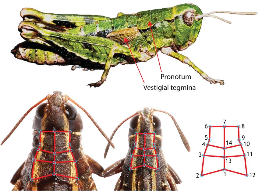
2   David Carmelet-Rescan et al.

(Excoffier et al., 2009). Coalescence of mtDNA haplotype diver-         signature of a sustained large population with high genetic diver-
sity within these expanding populations typically indicates            sity and connectivity. We did not expect to see concordance of
reduced population size during cold cycles, which is widely            morphological and genetic clusters, however environmental gra-
interpreted as the result of less habitat being available. However,    dients, fragmentation and the shared history of a non-
some species are likely to have found their preferred habitat was      recombining gene can naturally result in clusters that might have
shrinking during the interglacial rather than glacial phases           the appearance of multiple species. We did not expect the
(Lister & Stuart, 2008; Dong et al., 2017). Relatively small range     mtDNA diversity within this species to coalesce as recently as
shifts are typically inferred for species that are perceived as        the LGM when open habitat was available to support large popu-
tracking narrow elevational habitat zones on mountains                 lations of this insect.
(e.g. Schmitt, 2007; Gentili et al., 2015), but it could be the case
that cold-adapted species had larger populations and more con-
tinuous ranges during comparatively lengthy cold periods               Methods
(Dergachev, 2015). Alpine specialists tend to be restricted in dis-
tribution to higher latitudes and/or fragmented high elevation         Sampling
habitats, but they might retain high genetic diversity from larger
populations in the recent glacial past. Signatures of gene flow            We collected S. australis grasshoppers from 27 locations in
may remain from when their populations were not isolated on            South Island New Zealand, extending the documented range of
mountain peaks.                                                        this species (Figure 1; Supporting Information Table S1.1).
   Our modern anthropogenic perspective is from the situation of       Grasshoppers were collected by hand in subalpine and alpine
an interglacial climate, but prevailing conditions have existed for    habitat on mountains of the Southern Alps when grasshoppers
a relatively short time (Dergachev, 2015), whereas colder ‘gla-        were active during the New Zealand summer (December to
cial’ climate persisted up to 10 times longer with continuous          March, 1995–2016; Trewick, 2008; Trewick & Morris, 2008;
change operating in cycles. Glacial phases increased the relative      Dowle et al., 2014). The majority of specimens came from hab-
extent of alpine habitats in temperate and montane areas               itat between 1100 and 1890 m asl, but rare low elevation
(Birks, 2008) and also grasslands in subtropical regions               (~300 m asl) populations were also sampled. Specimens were
(Piñeiro et al., 2017). In contrast, ongoing anthropogenic global      frozen before immersion in 95% ethanol, and identification fol-
heating (Steffen et al., 2018) can only attenuate an already atyp-     lowed Bigelow (Bigelow, 1967). Maturity and sex were assessed
ical situation in terms of planetary climate in the Quaternary, and    using size and shape of terminalia and tegmina, and recorded
perhaps since the mid-Miocene disruption (Holbourn                     along with date, elevation and location (recorded using a porta-
et al., 2018). The insular nature of alpine systems, which contain     ble GPS device).
a disproportionate amount of terrestrial biodiversity (Rahbek
et al., 2019), makes them especially vulnerable to biological ero-
sion and significant in terms of ecosystem processes (Trisos            Niche modelling
et al., 2020).
   Here, we use analysis of changing conditions in the Southern           To estimate the environmental envelope suitable for S. australis,
Alps, New Zealand (Ka Tiritiri o te Moana, Aotearoa) to infer         location records were acquired for 14 species of New Zealand
population level effects, focussing on the flightless alpine-           endemic grasshoppers (Supporting Information Fig. S1.1).
adapted grasshopper Sigaus australis which is common above             Including multiple species increases the accuracy of our niche
the tree line. The Southern Alps extend across almost 5 of lati-      models by providing reliable absence information. Records from
tude making a nice system for investigation of elevation and lat-      our collection, journal articles, books and Crown Pastoral Lease
itude gradients. The geology and biology of the area at the            Tenure Reviews (produced by Land Information New Zealand)
juncture of two tectonic plates (Trewick et al., 2007) is well         were compiled with data from our own grasshopper collections
explored. Today about 50% of South Island is elevated above            (Supporting Information Table S1.2). All observations were
500 m and more than 20% is above 1000 m providing habitat              included in a binary table where the presence or absence of
for a rich alpine biota (e.g. Halloy, & Mark, 2003; Koot               S. australis was recorded for each location.
et al., 2020). Using niche models based on the current fragmen-           In order to define and project the potential niche of
ted distribution of S. australis, we examined whether the envi-        S. australis, 19 Bioclimatic variables were obtained from the
ronmental envelop of this species would have been more                 Worldclim website (Hijmans et al., 2005) for two different time
widespread and with greater connectivity during the LGM. We            periods – the LGM(c. 30–8 ka), and ‘current’ (data averaged
considered the extent of glacial ice and fragmentation of past         from 1960 to 1990; Supporting Information Table S1.3). Climate
and current habitat. Seeking evidence that S. australis distribu-      layers were produced using the MIROC-ESM global climate
tion was formerly more contiguous, we surveyed the species             model (Watanabe et al., 2011), at a resolution of 2.5 arc minutes
looking for evidence of gene flow during the LGM in the form            for the LGM and 30 arc-seconds for the current layer. The
of isolation by distance, using pronotum shape and mtDNA var-          Worldclim files were cropped to the extent of New Zealand
iation. The process of divergence with gene flow would leave a          (Latitudes: −49, −32; Longitudes: 165, 180) using QGIS
signature of isolation by distance and might result in a correla-      (QGIS Development Team, 2016). A variance inflation factor
tion between phenotypic and genetic distance. The availability         (VIF) (Lin et al., 2011) analysis was used in a stepwise selection
of widespread suitable habitat during the LGM would leave a            process to identify and remove collinear variables and reduced
                                    © 2021 Royal Entomological Society., Insect Conservation and Diversity, doi: 10.1111/icad.12488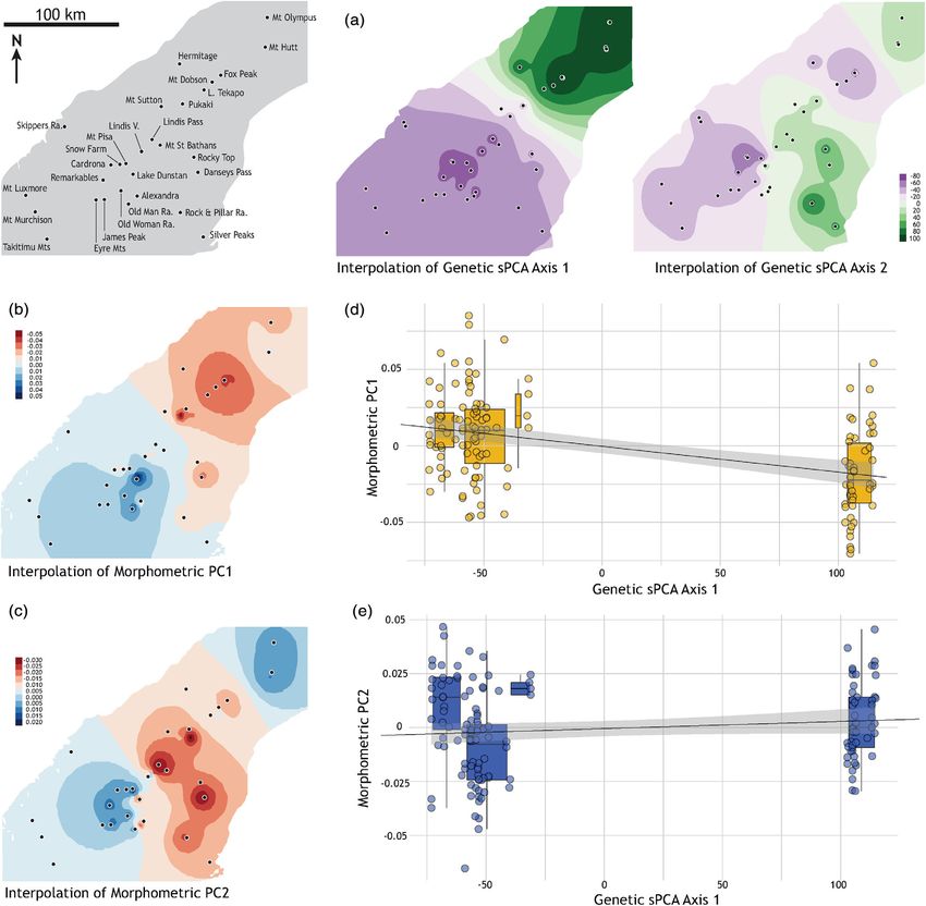
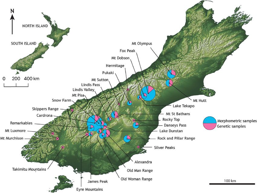
Spatial pattern in an alpine grasshopper        3

Figure 1. Sample locations for specimens of the alpine grasshopper Sigaus australis in South Island, New Zealand, used in morphometric and genetic
analysis. Pie segments represent the proportion of each type of sample and their size represents relative sample size. [Color figure can be viewed at
wileyonlinelibrary.com]

the list of 19 climate variables down to seven using the R pack-             to the niche model under current conditions and were therefor
age usdm (Naimi et al., 2014) and a threshold of 10 (Supporting              retained for model prediction with LGM climate estimates. As
information Table S1.3). By removing variables with strong cor-              soils associated with the Southern Alps form quickly and are
relation we minimised over-fitting and increase parsimony dur-                dominated by weathering of rapidly uplifting rock strata
ing the modelling process (Fletcher et al., 2016).                           (Larsen et al., 2014), it is probable that climate cycling influ-
   Soil and vegetation layers were included in the analysis                  ences the rate of formation but not characteristics of the soil.
because these two environmental variables are known to influ-                    To estimate the environmental niche of S. australis, we used
ence the distribution of some grasshopper species (Nattier                   the R package biomod2 v. 3.3-7 to apply 10 different modelling
et al., 2013; Weiss et al., 2013). Soil and vegetation data layers           methods to the presence and absence data of the grasshoppers in
were rasterised, clipped and re-scaled to a resolution of 30 arc-            the context of ‘current’ predictor variables (Thuiller et al., 2016).
seconds from their original files Fundamental Soil Layers                     Default modelling parameters were used with 80% of the data to
New Zealand Soil Classification and Vegetative Cover Map of                   calibrate the models and then tested with remaining 20%. Each
New Zealand, obtained through the Land Resource Information                  model was repeated three times resulting in a total of 30 models.
System (LRIS) portal (Leathwick et al., 2012). These layers rep-             Output values of variable importance were calculated as 1 minus
resent the current approximate state of vegetation and soil in               the mean correlation score of each variable, with scores closest to
New Zealand and were therefore used as static layers throughout              1 indicating a variable of high importance. Investigation of
the modelling process. In the absence of a verified model of                  model accuracy was carried out using two different evaluation
New Zealand soil and vegetation cover during LGM, Ecological                 methods: receiver operating characteristic (ROC) [i.e. area under
Niche Models that include static layers of this type are known to            the curve (AUC)] and true skill statistic (TSS). Models with
perform as well as, or better than, models where only dynamic                ROC values of 0.9–1 and TSS values of 0.8–1 are considered
variables are included (Stanton et al., 2012). Inclusion of these            to have ‘excellent’ predictive power (accuracy) (Thuiller
static layers enabled exploration of their potential contribution            et al., 2009). An ensemble model was then generated from a
© 2021 Royal Entomological Society., Insect Conservation and Diversity, doi: 10.1111/icad.12488
4   David Carmelet-Rescan et al.

subset of these models based on their ROC values (>0.8). Using         structure is not susceptible to arbitrary changes during preserva-
the ensemble model, ensemble forecasts were projected for the          tion (Friedrich et al., 2014). The shape of the posterior margin of
LGM. Plots were produced for each time period using the                the pronotum provides diagnostic differences that distinguish
Ensemble Model mean weights model (EMmw). EMmw                         many of the New Zealand grasshopper species and have previ-
variable importance was calculated by applying the weights pro-        ously been shown to be amenable to geometric morphometric
duced in the ensemble model to the associated models in the            approaches (Dowle et al., 2014; Ober & Connolly, 2015). Shape
30 model data set. Models were run three times for each predictor      was analysed using two-dimensional landmark-based geometric
variable, these were then averaged and EMmw variable impor-            morphometrics (Webster & Sheets 2010). Grasshoppers were
tance was calculated by summing the total of the averages for          arranged with pronotum perpendicular (horizontal) to the camera
each predictor variable, and dividing by the number of modelling       lens axis (Figure 2). Images were taken using a Canon EOS Kiss
methods used (i.e. 10) (Fletcher et al., 2016). Final scores of var-   X5 (600D) with EF100 mm f2.8 USM macro lens 1:2 mounted
iable importance were converted into percentages of total vari-        on a vertical stand (Kaiser). Digital images were organised into
able importance for each modelling method.                             thin plate spline (TPS) files using tpsUtil (Klingenberg, 2013;
   Binary vectors of each ensemble model were generated for            Rohlf, 2015) and landmarks were digitised and scale-calibrated
range change and fragmentation statistical analyses. These             using tpsDig2 on a Wacom Cintiq 22HD Pen Display tablet.
binary vectors were generated from the EMmw model dataset,             All photography and landmark positioning was done by one per-
where each pixel that scored greater than the predetermined            son to minimise operator error.
cut-off value was ranked as a 1, and all other pixels as 0’s. In          Analysis of shape variation used 14 landmarks identified
order to compare the binary vectors, LGM binary vector was dis-        around the perimeter and the dorsal surface of the pronotum
aggregated to correspond with the resolution of current binary         on each image of 503 grasshoppers. Landmarks 1, 2, 6, 8 and
vector using the R package raster (Hijmans & Etten, 2012).             12 relate to the main angles of the pronotum dorsal perimeter,
When comparing binary vectors between current and past                 13 and 14 are at the intersection of sulci (surface grooves) with
models, Biomod2 ranked pixels as: ‘Never occupied’                     the dorsal midline, 3, 4, 5, 9, 10 and 11 on the lateral carinae
(i.e. pixels were unoccupied and remain unoccupied between             (Fig. 2). X and Y coordinates are then assigned to each land-
models), ‘Always occupied’, ‘Lost’ (i.e. pixels were occupied          mark. Generalised Procrustes analysis (Goodall, 1991;
but become unoccupied in the current model) or ‘Gained’                Bookstein, 1992) was run using the R package geomorph
(i.e. pixels that were unoccupied in the LGM model become              v3.0.5 (Adams et al., 2017) in the R statistics environment
occupied in the Current model), from which range change statis-        (R Core Team, 2019). Non-shape variation was therefore math-
tics were then calculated.                                             ematically removed as position, orientation and size superim-
   As the LGM was characterised in New Zealand by the exten-           poses landmark configuration using least-squares estimates
sion of valley glaciers that would limit the occupation of poten-      for translation and rotation (Adams et al., 2013; Webster &
tial habitat predicted by the climate modelling we examined its        Sheets, 2010). We examined error associated with image cap-
extent using the results of a geomorphological analysis (James         ture using Procrustes ANOVA with 1000 permutations
et al., 2019). Predicted ice cover of ~6800 km3 during LGM             (Anderson & Braak, 2003). This analysis allowed estimation
was implemented on the binary vectors excluding the pixels             of repeatability using the interclass correlation coefficient
overlain by the ice cover layer from James et al. (2019). We           (Fruciano, 2016) and revealed that the error arising from image
improvised uncertainty about glacier margins and seasonal fluc-         capture and landmark positioning variation was biologically
tuations by iterating the analysis with the exclusion of the pixels    irrelevant: the repeatability is above 90% (93.7%) using 30 indi-
of the binary vector where the ice layer was predicted to be over      viduals for landmark positioning and 18 individuals for image
50 m and 100 m. Fragstats, implemented in the R package SDM            capture.
Tools v 1.1–221 (VanDerWal et al., 2012), also used these                 Size-corrected shape was produced from residuals of the Pro-
binary files to estimate fragmentation statistics (e.g. patch size,     crustes ANOVA against centroid size after revealing that prono-
number of patches), which were compared between LGM and                tum size have an impact on shape despite the Procrustes
current niche models. For each scenario pixels that were con-          superimposition (Gould, 1966; Klingenberg, 2016). The pack-
nected within each of the binary files were given unique patch          age geomorph also implements MANCOVA, an analysis of var-
identities, and the area these patches calculated. The total area      iance of several dependent variable (landmarks coordinates) by
and the number of patches into which that area was distributed         level of an independent factor variable, such as the population
were computed excluding the smaller patches. We used a range           or the sex of each individual, and covariation of linear indepen-
of exclusion thresholds (from 250 km2 to 3000 km2) allowing            dent variables such as latitude (Collyer et al., 2015).
us to investigate habitat connectivity indicated by different             Principal components analysis (PCA) of the pronotum shape
scenarios.                                                             and size-corrected pronotum shape variation from the covariance
                                                                       matrix of the X-Y coordinates were performed using the geo-
                                                                       morph package. The principal components generated by PCA
Phenotypic variation                                                   reflect (mathematically) independent variation in the shape of
                                                                       objects, and centroid size acts as a proxy for size variation (inde-
   To explore morphological variation within and between popu-         pendent of shape). Statistically significant principal components
lations, we used a geometric morphometric approach. Pronotum           (PCs) were identified using the broken-stick test on eigenvalues
shape variation was used as a proxy for overall variation as this      to identify PCs that explain more variance in the data than
                                    © 2021 Royal Entomological Society., Insect Conservation and Diversity, doi: 10.1111/icad.12488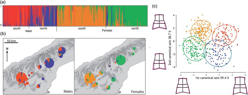
Spatial pattern in an alpine grasshopper          5

Figure 2. Phenotypic variation of the New Zealand alpine grasshopper Sigaus australis was quantified using geometric morphometric shape analysis
with 14 landmarks arranged on the dorsal surface of the pronotum. Adult female green form (top), and anterior dorsal view of female (left) and male (cen-
tre) to the same scale with landmark array (right). [Color figure can be viewed at wileyonlinelibrary.com]

expected by chance alone, implemented in the R package vegan                    groups (sex and geographic location) using the Mahalanobis dis-
2.2 (Oksanen et al., 2018). Geographic correlation of shape                     tance (Campbell & Atchley, 1981; Klingenberg, 2013).
between populations was tested using the significant principal
components from the morphometric analysis to compute mor-
phometric distance between individuals (Euclidian distance).                    Phylogeography
Then the inter-population morphometric distance between two
populations was computed by summing the distances for pairs                        The mitochondrion remains the locus of choice for intraspecific
of individuals from two different population and dividing this                  animal phylogeography because it is single copy, uniparental and
value by the number of sum computed (Dellicour et al., 2017).                   nonrecombining; this allows robust inferences about genealogy
The resulting distance matrix was then compare to the geograph-                 (Avise, 1986; DeSalle et al., 2017). Here, we utilised the ND2
ical distance of population using a Mantel test (Mantel, 1967),                 (NADH dehydrogenase 2) gene to estimate S. australis genealogical
with 1000 bootstrap replicates.                                                 relationships as it has a higher capacity to accumulate haplotype
   Model-based assignment analyses were computed using sig-                     diversity than the commonly analysed COI locus (Koot et al., 2020).
nificant principal components from the PCA on the pronotum                          Whole genomic DNA was extracted from muscle tissue from
shape + centroid size with the R package Mclust 5.4 (Scrucca                    hind femora of 195 grasshopper specimens using a solvent-free
et al., 2016). This uses an iterative expectation–maximisation                  Proteinase K and salting-out method (Sunnucks & Hales, 1996)
(EM) method with Gaussian mixture modelling (Fraley &                           as previously described (Sivyer et al., 2018). Polymerase
Raftery, 2002) with model selection using Bayesian information                  chain reaction used standard conditions with ND2 primers
criterion (BIC) scores. Variables are scaled because size is used               HopND2_147F (5’ TGACCAACAACTCTACAAAACTTCT
as a variable and the Mclust algorithm assumes the same vari-                   3’) and HopND2_1286R (5’ TCAATAATGATTCTAGACTG-
ance across all variables. To evaluate whether clustering results               CAATTCT 3’) (Koot et al., 2020). Sequencing used BigDye
can be related to an actual grouping an adjusted Rand index is                  v3.1 chemistry and an ABI3730 DNA analyser with results edited
run. The adjusted Rand index compares the two partitions and                    and aligned in Geneious R10 (Kearse et al., 2012). Population
has an expected value of 0 in the case of random partition, and                 genetic analysis was conducted using statistical language R
it is bounded above by 1 in the case of perfect agreement                       (R Core Team, 2019) and various packages. Matrilineal genetic
between two partitions (Hubert & Arabie, 1985; Scrucca                          diversity within each population sample (n ≥ 5) was estimated
et al., 2016). Canonical variate analysis (CVA) with cross-                     by computing haplotype diversity (H) that represents the probabil-
validation score was performed on shape data (503 sets of land-                 ity that two randomly sampled haplotypes are different, and nucle-
mark coordinates) with the R package Morpho (Schlager, 2016).                   otide diversity (π), which is the average number of nucleotide
This analysis statistically tests the separation between defined                 differences per site in pairwise comparisons among DNA
© 2021 Royal Entomological Society., Insect Conservation and Diversity, doi: 10.1111/icad.12488
6 David Carmelet-Rescan et al.
sequences (Nei, 1987) using R package pegas (Paradis, 2010).
Matrilineal relationships were inferred using median-joining hap-
lotype networks (Bandelt et al., 1999) generated using PopART
(Leigh & Bryant, 2015) and the R package igraph (Csardi &
Nepusz, 2006), to represent the relationships between haplotypes
among populations. The haplotype network was computed under
haplotype pairwise differences, giving the number of substitution
steps between haplotypes.
Pairwise Φst values were computed to infer variation within
and among populations with significance deviations from zero
estimated by comparison with 1000 random permutations of
the data (Excoffier et al., 1992). Isolation by distance was
assessed using the Mantel test (Mantel, 1967; Tamura &
Nei, 1993) comparing pairwise population Φst and Euclidian dis-
tances between geographic coordinates with 1000 bootstrap rep-
licates. To investigate the correlation between genetic and
morphometric variation we used a Mantel test between pairwise
genetic distance and a morphometric PCA distance matrix with
144 individuals specimens for which we had both data. We
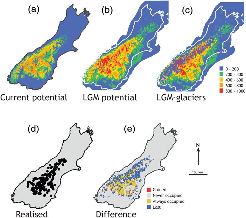
visualised the correlation using spatial principal components Figure 3. The realised niche space of the alpine grasshopper Sigaus
analysis (sPCA) with the genetic data using the R package ade- australis in South Island, New Zealand alongside their potential niche
genet (Jombart, 2008) and mapped an interpolation of genetic spaces predicted using Ensemble Model Mean Weights models.
sPCA and morphometric PCA first two axis values. (a) Predicted suitable niche space for current climate. (b) Predicted
potential niche space during the Last Glacial Maximum (LGM) including
inferred land extension. (c) As in B subtracting areas covered by valley
Results glaciers. (d) Known current occurrence of S. australis. (e) Difference in
potential habitat between LGM (no ice) and current climate models gen-
erated by comparing binary vector layers of LGM and current ENMs for
Niche modelling
pixels with score above threshold of 536.5. [Color figure can be viewed
at wileyonlinelibrary.com]
S. australis was present at 278 of the 963 locations where grass-
hoppers were recorded and used to estimate the environmental
envelope for the species. Most models had high receiver operating extent of suitable environment during the LGM suggests
characteristics (ROC > 0.8; Supporting Information Fig. S1.2), S. australis could have had a wider range (36 359 km2) in the past
and the EMmw ensemble model had an improved ROC (0.917) than today (16 661 km2) (Fig. 3; Table 1). However, when the
compared to individual models. Sensitivity (percentage of pres- estimated extent of valley glaciers was considered the estimated
ences correctly predicted) and specificity (proportion of absences potential habitat during LGM was reduced substantially
predicted; Allouche et al., 2006) of the EMmw model were 75.9% (Fig. 3c). At maximum estimated extent, valley glaciers eliminate
and 88.3%, respectively. The cut-off threshold that maximised the habitat area gains (15,178 km2), although this impact is lessened
proportion of presences and absences correctly predicted by the with increasing allowance of edge ice thickness to accommodate
model used to produce binary vector layers was 536.5. Tempera- uncertainty of glacier limits, seasonal fluctuation and ice reduction
ture attributes had the largest (~70%) influence on the environ- post-LGM. Nevertheless, we inferred fewer large habitat frag-
mental envelope determined for S. australis. Annual mean ments in the current model (43% fragments >3000 km2) than dur-
temperature was the most important predictor variable (29.1% of ing the LGM (85% fragments >3000 km2), even if the full extent
importance), but mean diurnal range (22.4%) and mean tempera- of glaciers was considered (57% fragments >3000 km2). This pre-
ture of driest quarter (17%) were also important in explaining dicts a higher level of gene flow was possible across the species
presence of S. australis (Supporting Information Fig. S1.3). range during the LGM and that loss of genetic diversity due to
The environmental envelope was used to estimate total avail- drift would have been minimal. We sought evidence of this past
able habitat for S. australis at two time points (Fig. 3). The connectivity by examining the extent and distribution of pheno-
Potential Niche Space model for current conditions (Fig. 3a) cor- typic and genetic variation displayed by extant S. australis popu-
responded to the known distribution (Realised Niche Space, lations that are isolated from one another today.
Fig. 3d), suggesting that the distribution of S. australis is likely
constrained by the climate variables used in our models or that
these variables are close proxies for other important environmen-
tal traits. Temperature appears to be a factor limiting the distribu- Phenotype variation
tion of S. australis (Supporting Information Fig. S1.4).
We predicted where suitable niche space would have likely Pronotum shape of 490 adult S. australis specimens spanning
been available for this grasshopper lineage during the LGM using the current range was examined. A strong significant effect of
results from our initial current ENMs (Fig. 3b). The inferred wider sex on pronotum shape was detected (MANCOVA on Procrustes
© 2021 Royal Entomological Society., Insect Conservation and Diversity, doi: 10.1111/icad.12488Spatial pattern in an alpine grasshopper 7
Table 1. Available habitat for Sigaus australis predicted with EMmw niche model for current climate and conditions during the last glacial maximum
(LGM).
Current LGM LGM < 100 m ice LGM < 50 m ice LGM < 0 m ice
Min. patch size Total Ratio Total Ratio Total Ratio Total Ratio Total Ratio
>0 16661 1.00 36359 1.00 25825 1.00 22646 1.00 15178 1.00
>250 15258 0.92 36070 0.99 25458 0.99 22079 0.97 14932 0.98
>500 14875 0.89 35962 0.99 24931 0.97 21771 0.96 14652 0.97
>1000 14252 0.86 35591 0.98 24569 0.95 21480 0.95 14252 0.94
>3000 7097 0.43 30777 0.85 21186 0.82 15749 0.70 8653 0.57
Extension of valley glaciers during the LGM is accommodated by excluding potential habitat overlain by ice up to 100 m, 50 m and 0 m thick,
respectively. We sampled at habitat patch size intervals from 0 to 3000 km2 and calculated the proportion of total for each model contained within
fragments of each size range.
analysis of pronotum shape), which is consistent with visible sex- resolved four clusters of specimens with the best fitting model
ual dimorphism including size (Table 2(A)). Difference in prono- (EEE4: ellipsoidal, equal volume, shape and orientation model
tum shape between males and females decreased when we used a with four components). These clusters largely partition the per-
size-corrected shape analysis (Table 2(B)) revealing an allometric mutations of male, female, northern and southern grasshoppers
effect (Gould, 1966; Klingenberg, 2016). A significant effect of (Figure 4). The northern phenotype was common at Mt Olym-
latitude on shape variation was detected with pronota being nar- pus, Mt Hutt, Fox Peak, Danseys Pass, Pukaki, Lake Tekapo,
rower in northern versus southern individuals. A less pronounced Mt Dobson, Rock & Pillar Range, while the southern phenotype
narrowing of pronota with increasing elevation was also apparent. was common in Cardrona, Remarkables, Lake Dunstan, Snow
Despite the significance of sex, latitude and elevation as explana- Farm, Old Man Range, Lindis Pass, Old Woman Range, Lindis
tory variables, most shape variance (92%) was still unexplained Valley, Alexandra, James Peak and Mt Pisa (Fig. 4(B)).
(Table 2(B)). Using the four clusters resolved by Gaussian mixture model-
There were three significant principal components in the pro- ling, specimens were in general grouped with other specimens
notum shape data explaining 40.4% (PC1), 14.0% (PC2) and of the same sex and geographic location (north/south), but there
8.3% (PC3) of variation. A Mantel test revealed a significant were 81 misassignments out of 490 individuals (adjusted Rand
positive spatial correlation between pairwise morphological dis- index = 0.6474, 83.5% correct assignment). Most specimens
tance and geographic distance (Females, Z = 0.4515, were correctly assigned to sex on the basis of pronotum shape
P = 0.000999; Males, Z = 0.2308, P = 0.02298; Supporting (19 misassignments), but some grasshoppers from northern sites
Information Fig. S1.5). did not cluster with geographically adjacent individuals. In par-
Naive clustering (Gaussian mixture modelling) of pronotum ticular, we found several misassignments among male grasshop-
variation using three significant PCA components and size pers collected from Mt Olympus and Cardrona (approximately
40% of misassignments). Other geographically misassigned
grasshoppers were from sites between northern and southern
Table 2. Morphological variation within Sigaus australis using land- locations and from isolated population samples including
mark coordinates considering effect of sex, latitude and elevation on Rock & Pillar Range, Danseys Pass and Mt Hutt.
shape variation using Procrustes MANCOVA with 1000 permutations. Canonical variate analysis (CVA) on pronotum shape data
(A) Procrustes-aligned coordinates of pronotum landmarks and (B) showed separation between sex and between North and South
size-corrected Procrustes-aligned coordinates of pronotum landmarks individuals (classification accuracy: 88.98%) and allowed defi-
(A) d.f. SS MS F P
nition of the shape differences by a single component (Fig. 4
(C)). As each CVA axis mostly represents one factor in this case,
Sex 1 0.20022 0.200221 105.2278 David Carmelet-Rescan et al.
Figure 4. Phenotypic variation within Sigaus australis based on geometric morphometric analysis of pronotum shape. (a) Assignment probabilities of
grasshopper individuals to each of four clusters (represented by different colours) inferred naively by mclust with the optimal EEE4 model, arranged by
sex and region. Each bar represents assignment probability of one individual. (b) Spatial distribution of predominant cluster assignment of males and
females, where each pie represents a population sample location scaled by the number of individuals and each colour represent the proportion of each
cluster. (c) The first two axes of a canonical variates analysis on pronotum landmark coordinates with sex and region of origin defined a priori. Results
indicate that these categories are relevant to cluster shape and provide an explanation for the clustering result (88.98% of classification accuracy). Shape
differences gathered by each canonical axis are represented by the estimated pronotum shape for a high and low value of the canonical component. The
black landmarks are the estimated landmarks and pink is the consensus shape of the sample. [Color figure can be viewed at wileyonlinelibrary.com]
Information Table S1.4) and low in the smallest samples Discussion
(e.g. Lake Dunstan, Lake Tekapo and Remarkables). Nucleotide
site variation differed considerably among population samples, Of all the climatic and environmental variables included in our
ranging from 0 to 0.0347. models, we found temperature to be the most important factor
Few ND2 mitochondrial DNA haplotypes were shared among determining the presence or absence of the alpine grasshopper
population samples, and the overall ΦST was significantly S. australis in New Zealand. The key variables in our model are
greater than zero (0.8829, P < 0.001). In general, geographically likely to be proxies for a set of correlated variables that include
adjacent population samples had similar haplotypes and the low- temperature. Temperate grasshoppers need to bask in the sun
est pairwise ΦST estimates were observed when these neighbours (Koot et al., 2020), so their ranges in New Zealand are limited
were compared. Over the entire species range IBD was apparent to open habitats (Bigelow, 1967). In a landscape naturally domi-
with significant correlation between pairwise ΦST and geo- nated by wet forest (Trewick & Morgan-Richards, 2009), the ele-
graphic distance (Mantel test; Z = 0.2299, P = 0.01898, Support- vational tree line is the major constraint on the distribution of such
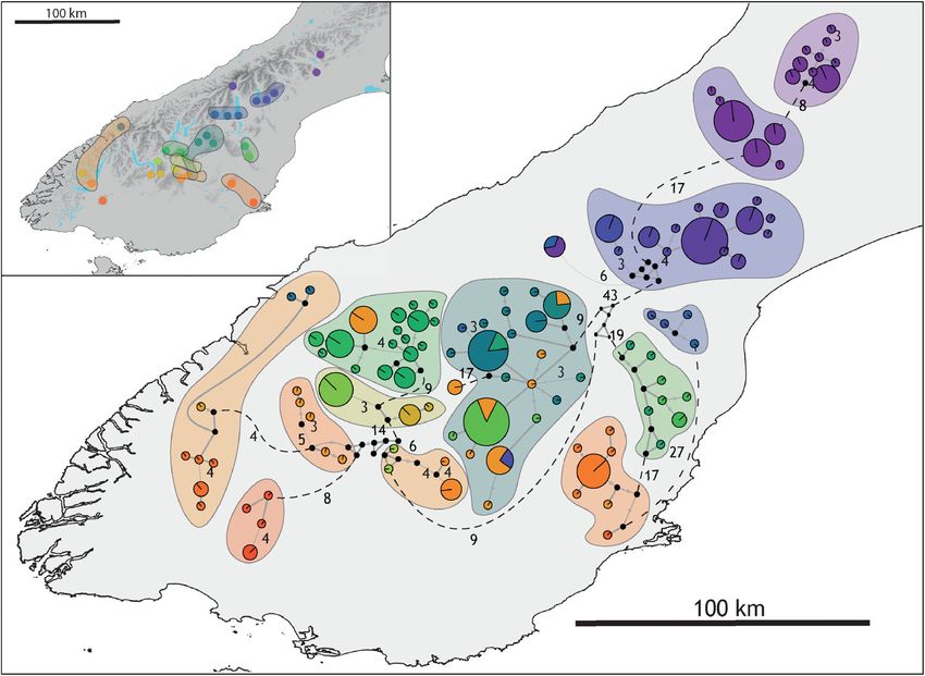
ing Information Fig. S1.6). Major haplotype clusters within habitat and is itself primarily controlled by temperature
S. australis were apparent between the most northern population (Körner, 1998). As a result, climate cycling during the Pleistocene
samples (Mt Olympus, Mt Hutt, Lake Tekapo, Mt Dobson and was characterised by substantial shifts in both the latitudinal and
Fox Peak) and all others and were separated by more than elevational extent of forest and open habitat. The cooling and
50 nucleotide substitutions (Fig. 5). attendant aridification experienced globally during Pleistocene
cold phases was locally emphasised in South Island,
New Zealand where the Southern Alps cast an eastern rain-
shadow that extended available open habitat (Ausseil et al., 2011).
Despite this, our modelling indicates that total habitat area
Concordance of genetic and phenotypic clusters available to S. australis during the LGM was probably similar
to the present. Although the estimated LGM environmental
We found a significant correlation between morphometric PCA envelop was more than twice that available today, valley glaciers
distance and genetic distance using a Mantel test among individ- comprising about 100 times as much ice as they currently do,
uals common to these datasets (n = 144, Z = 0.1589, P = 0.001; obscured more than half of this. Nonetheless, our models suggest
Supporting Information Fig. S1.7). The broad correlation of shape that S. australis populations were less fragmented during the
and lineage is apparent from the interpolation of genetic sPCA and LGM than experienced by their current high elevation distribu-
the first two morphometric PCA axes (Fig. 6), especially between tion. As S. australis (and all other endemic alpine grasshoppers;
the first axis of PCA and the first axis of sPCA. Koot et al., 2020) have vestigial tegmina (Fig. 2) and cannot fly,
© 2021 Royal Entomological Society., Insect Conservation and Diversity, doi: 10.1111/icad.12488Spatial pattern in an alpine grasshopper 9 Figure 5. MtDNA ND2 haplotype phylogeography of Sigaus australis grasshoppers. Median-joining haplotype network overlain on population sample locations. Nodes represents haplotypes and are colour-matched with their sample membership proportional to pie size. Edges represent minimum genetic distance between most similar haplotypes with number of substitutions between linked nodes displayed. Inset shows location sample sites coloured by predominant ND2 cluster. [Color figure can be viewed at wileyonlinelibrary.com] mountain populations are reproductively isolated from one populations, is counter to the high intraspecific genetic diversity another by the tree line that responds to mountain shape and detected in many alpine species (e.g. Pauls et al., 2006; Bettin other variables (Case & Buckley, 2015). In contrast, during the et al., 2007). Generally, high genetic diversity is considered indic- considerably longer glacial periods (each ~100 kya) gene flow ative of large populations (Charlesworth, 2009), and this is borne for ‘alpine’ species was less constrained. out in alpine habitats by demographic analyses (e.g. Huang Interpretation of alpine phylogeography has followed from et al., 2016). Therefore, reference to range change rather than the findings made of low elevation biota that identified popula- ‘refugia’ is more appropriate as it avoids the implication that the tion refugia during the colder periods of the Pleistocene current climatic situation represents the norm. (Taberlet et al., 1998; Hewitt, 2000). Indeed, population expan- Among New Zealand alpine species, high intraspecific genetic sion from glacial refugia has also been proposed for some north- diversity observed in populations with small modern ranges ern hemisphere alpine species including grasshoppers with probably reflects large populations sustained throughout the limited intraspecific diversity (Knowles, 2000; Berger Pleistocene (e.g. Trewick et al., 2000; King et al., 2003; McCul- et al., 2010). This suggests such species were rarer in glacial than loch et al., 2009; O’Neill et al., 2009). A similar situation is inter-glacial phases of the Pleistocene. One explanation offers observed in Australian mountains (e.g. Endo et al., 2015). From nunataks (ridges protruding between glaciers) as micro-refugia this, we infer that any loss of potential range for cold-adapted, during glaciation by referencing modern conditions and does open-habitat specialists is most likely to have occurred during predict reduction in available habitat for alpine adapted taxa. relatively short interglacials rather than glacials (Sivyer Data, however, do not strongly favour this interpretation et al., 2018). In S. australis grasshoppers, we find better support (e.g. Rogivue et al., 2018; Zhang et al., 2018). for more continuous range in the LGM than for alternative Given inferences of range shifts in populations of low eleva- hypotheses of isolated nunatak refugia. Grasshoppers in south- tion taxa during Pleistocene glacial phases, it is implicit that western populations (e.g. Skippers Range, Takitimu Mountains) alpine-like conditions extended at the same time. This wider that are today isolated from others in the Southern Alps, are most availability of open habitats in the northern hemisphere is, for similar to grasshoppers in nearby south central habitat. In con- instance, demonstrated by phylogeographic signal from mam- trast, eastern central populations (e.g. Danseys Pass, Rock and moth remains (Palkopoulou et al., 2013). The idea that alpine Pillar Ranges) represent a more deeply diverged mtDNA lineage taxa might have been subject to ‘glacial refugia’ (Holderegger & consistent with unglaciated habitat continuity during the LGM. Thiel-Egenter, 2009), implying LGM range restriction and small High haplotype diversity within the central area (e.g. Lindis © 2021 Royal Entomological Society., Insect Conservation and Diversity, doi: 10.1111/icad.12488
10   David Carmelet-Rescan et al.

Figure 6. Comparison between geometric morphometric and genetic clustering of Sigaus australis alpine grasshoppers (n = 141). (a) Interpolation of
first and second axes of spatial PCA on ND2 mtDNA haplotypes. (b) Interpolation of first axis of PCA of pronotum shape. (c) Interpolation of second
axis of PCA of pronotum shape. (d) First axis of sPCA on ND2 against first axis of PCA of pronotum shape. Boxplots created with a bin width of
20, and linear regression with 95% confidence interval in grey. (e) First axis of sPCA on against second axis of PCA of pronotum shape. [Color figure
can be viewed at wileyonlinelibrary.com]

Valley, Lake Dunstan) associated with low elevation semi-arid                diversity might result from biological artefacts (Hurst & Jig-
habitat suggests admixture (Dowle et al., 2014; Sivyer                       gins 2005), it is also the well-understood result of large popula-
et al., 2018). We have investigated genetic divergence using a               tion size (Morgan-Richards et al., 2017).
single non-recombining locus that represents the matrilineal his-               Niche models are limited by data, and the distribution of suit-
tory of the species efficiently and effectively (DeSalle                      able habitat needs to be considered as well as total size inferred
et al. 2017) and is especially informative when accompanied                  from climate models. The inferred area of suitable habitat for
by other types of information such as our morphometric analysis              S. australis during the LGM based on a niche model, that
(Rubinoff & Holland 2005). Although high mtDNA genetic                       assumes the grasshopper’s environmental requirements have
                                     © 2021 Royal Entomological Society., Insect Conservation and Diversity, doi: 10.1111/icad.12488
Spatial pattern in an alpine grasshopper 11
not substantially changed, was more than twice the size of our sequence alignments and distribution data will be deposited on
estimates that also considered the LGM distribution of montane Dryad (doi:10.5061/dryad.wh70rxwk8).
glaciers in New Zealand. After excluding the potential habitat
likely to have been covered by ice during the LGM reduced
our estimate of the past S. australis habitat to slightly less than Supporting information
the current potential habitat. MtDNA diversity detected in
S. australis was high and mostly partitioned among population Additional supporting information may be found online in the
samples, suggesting that S. australis populations have not Supporting Information section at the end of the article.
expanded from small glacial refugia but have remained large.
Our knowledge of Milankovitch cycles suggests that habitat suit- Appendix S1: Supporting Information
able for S. australis would have fluctuated many times, being
smallest during the warm and cold maxima, and larger as the cli-
mate cycled between. However, it appears unlikely that at any References
time would habitat and population size have reduced sufficiently
for mtDNA coalescence, thus maintaining high intraspecific Adams, D. C., Collyer, M., Kaliontzopoulou, A., & Sherratt, E. (2017)
diversity at this locus. Importantly, our niche models for Geomorph: geometric morphometric analyses of 2D/3D landmark
S. australis led us to infer that their past populations would have data. R Package Version 3.0.3.
been less fragmented during the LGM compared to their current Adams, D.C., Rohlf, F.J. & Slice, D.E. (2013) A field comes of age: geo-
distribution. Local differentiation with gene flow will lead to an metric morphometrics in the 21st century. Hystrix Italian Journal of
intraspecific population structure of isolation by distance if dis- Mammalogy, 24, 7–14.
persal is limited by geographical distance (Slatkin, 1993). The Allouche, O., Tsoar, A. & Kadmon, R. (2006) Assessing the accuracy of
current patterns of isolation by distance detected in presumably species distribution models: prevalence, kappa and the true skill statis-
tic (TSS). Journal of Applied Ecology, 43, 1223–1232.
neutral pronotum shape and limited mtDNA variation indicate
Anderson, M. & Braak, C.T. (2003) Permutation tests for multi-factorial
gene flow among populations in the recent past. Thus, in this analysis of variance. Journal of Statistical Computation and Simula-
flightless grasshopper, we see a signature of population connec- tion, 73(2), 85–113.
tivity from the LGM although many populations are today iso- Ausseil, A.G.E., Dymond, J.R. & Weeks, E.S. (2011) Provision of natu-
lated from one another at high elevation. Connectivity of ral habitat for biodiversity: quantifying recent trends in New Zealand.
populations during cool phases has probably prevented specia- Biodiversity Loss in a Changing Planet. (ed. by O. Grillo and G.
tion during short warm phases when populations are more frag- Venora), pp. p. 201–220.InTech, Rijeka.
mented. We detected some evidence of divergence between Avise, J.C. (1986) Mitochondrial DNA and the evolutionary genetics of
populations with a north/south distribution but half of our popu- higher animals. Philosophical Transactions of the Royal Society of
lation samples were polymorphic, and phenotype and mtDNA London B Biological Sciences, 312(1154), 325–342.
Bandelt, H.J., Forster, P. & Rohl, A. (1999) Median-Joining networks for
was not strictly concordant. Current predictions of global warm-
inferring intraspecific phylogenies. Molecular Biology and Evolution,
ing will shrink habitat resulting in reduction of population size, 16(1), 37–48.
further fragmentation and potential local extinction. The high Berger, D., Chobanov, D.P. & Mayer, F. (2010) Interglacial refugia and
genetic and phenotypic variation within S. australis might range shifts of the alpine grasshopper Stenobothrus Cotticus
enhance potential for adaptive response to the challenging cli- (Orthoptera: Acrididae: Gomphocerinae). Organisms Diversity and
matic changes, but loss of open alpine habitat to expanding forest Evolution, 10(2), 123–133.
at higher elevations will cause S. australis and other alpine spe- Bettin, O., Cornejo, C., Edwards, P.J. & Holderegger, R. (2007) Phylo-
cialists to decline. Future climate warming is likely to further geography of the high alpine plant Senecio halleri (asteraceae) in the
fragment and reduce population sizes and connectivity of all european alps: in situ glacial survival with postglacial stepwise dis-
cold-adapted species. persal into peripheral areas. Molecular Ecology, 16(12), 2517–2524.
Bigelow, R.S. (1967) Grasshoppers (Acrididae) of New Zealand; Their
Taxonomy and Distribution. University of Canterbury, Christchurch.
Birks, H.H. (2008) The late-Quaternary history of arctic and alpine
Acknowledgements plants. Plant Ecology and Diversity, 1(2), 135–146.
Bookstein, F.L. (1992) Morphometric Tools for Landmark Data. Cam-
The authors are grateful to the New Zealand Department of Con- bridge University Press, Cambridge.
servation for granting access and approval to collect from the Campbell, N.A. & Atchley, W.R. (1981) The geometry of canonical var-
Conservation Estate. The authors thank the ski field managers iate analysis. Systematic Biology, 30(3), 268–280.
who allowed us access to field sites: Jo Rainey at Rainbow Ski Case, B.S. & Buckley, H.L. (2015) Local-scale topoclimate effects on
Area, Gary Patterson at Fox Peak Ski Area, James McKenzie treeline elevations: a country-wide investigation of New Zealand’s
southern beech treelines. PeerJ, 3, e1334.
at Mt Hutt, and Erik Barnes at Cardrona Alpine Resort. Addi-
Charlesworth, B. (2009) Effective population size and patterns of molec-
tional grasshoppers were provided by Danilo Hegg and Eddy
ular evolution and variation. Nature Review Genetics, 10, 195–205.
Dowle. This research was assisted by a grant from the Miss Collyer, M.L., Sekora, D.J. & Adams, D.C. (2015) A method for analysis
E. L. Hellaby Indigenous Grasslands Research Trust. of phenotypic change for phenotypes described by high-dimensional
Data Availability Statement data. Heredity, 115(4), 357–365.
All mtDNA sequences were deposited in GenBank Csardi, G. & Nepusz, T. (2006) The igraph software package for com-
(MT712921 - MT713114). Geometric morphometric datasets, plex network research. InterJournal, Complex Systems, 1695(5), 1–9.
© 2021 Royal Entomological Society., Insect Conservation and Diversity, doi: 10.1111/icad.1248812 David Carmelet-Rescan et al.
Dellicour, S., Gerard, M., Prunier, J.G., Dewulf, A., Kuhlmann, M. & Holbourn, A.E., Kuhnt, W., Clemens, S.C., Kochhann, K.G.D.,
Michez, D. (2017) Distribution and predictors of wing shape and size Jöhnck, J., Lübbers, J. & Andersen, N. (2018) Late Miocene climate
variability in three sister species of solitary bees. PLOS ONE, 12(3), cooling and intensification of southeast asian winter monsoon. Nature
e0173109. Communications, 9(1), 1–13.
Dergachev, V.A. (2015) Length of the current interglacial period and Holderegger, R. & Thiel-Egenter, C. (2009) A discussion of different
interglacial intervals of the last million years. Geomagnetism and Aer- types of glacial refugia used in mountain biogeography and phylogeo-
onomy, 55(7), 945–952. graphy. Journal of Biogeography, 36(3), 476–480.
DeSalle, R., Schierwater, B. & Hadrys, H. (2017) MtDNA: the small Huang, C.C., Hsu, T.W., Wang, H.V., Liu, Z.H., Chen, Y.Y., Chiu, C.T.,
workhorse of evolutionary studies. Frontiers Bioscience (Landmark Huang, C.L., Hung, K.H. & Chiang, T.Y. (2016) Multilocus analyses
Ed), 22, 873–887. reveal postglacial demographic shrinkage of Juniperus morrisonicola
Dong, F., Hung, C.H., Li, X.L., Gao, J.Y., Zhang, Q., Wu, F., Lei, F.M., (Cupressaceae), a dominant alpine species in Taiwan. PLoS one, 11
Li, S.H. & Yang, X.J. (2017) Ice Age unfrozen: severe effect of the last (8), e0161713.
interglacial, not glacial, climate change on east asian avifauna. BMC Hubert, L. & Arabie, P. (1985) Comparing partitions. Journal of Classi-
Evolutionary Biology, 17(1), 244. fication, 2(1), 193–218.
Dowle, E.J., Morgan-Richards, M. & Trewick, S.A. (2014) Morpholog- Hurst, G.D. & Jiggins, F.M. (2005) Problems with mitochondrial DNA
ical differentiation despite gene flow in an endangered grasshopper. as a marker in population, phylogeographic and phylogenetic studies:
BMC Evolutionary Biology, 14(1), 216. the effects of inherited symbionts. Proceedings of the Royal Society B:
Endo, Y., Nash, M., Hoffmann, A.A., Slatyer, R. & Miller, A.D. (2015) Biological Sciences, 272(1572), 1525–1534.
Comparative phylogeography of alpine invertebrates indicates deep James, W.H.M., Carrivick, J.L., Quincey, D.J. & Glasser, N.F. (2019) A
lineage diversification and historical refugia in the Australian alps. geomorphology based reconstruction of ice volume distribution at the
Journal of Biogeography, 42(1), 89–102. Last Glacial Maximum across the Southern Alps of New Zealand.
Excoffier, L., Smouse, P.E. & Quattro, J.M. (1992) Analysis of molecu- Quaternary Science Reviews, 219, 20–35.
lar variance inferred from metric distances among DNA haplotypes: Jombart, T. (2008) Adegenet: a R package for the multivariate analysis of
application to human mitochondrial DNA restriction data. Genetics, genetic markers. Bioinformatics, 24(11), 1403–1405.
131(2), 479–491. Kearse, M., Moir, R., Wilson, A., Stones-Havas, S., Cheung, M.,
Excoffier, L., Foll, M. & Petit, R.J. (2009) Genetic consequences of Sturrock, S., Buxton, S., Cooper, A., Markowitz, S., Duran, C.,
range expansions. Annual Review of Ecology, Evolution, and System- Thierer, T., Ashton, B., Meintjes, P. & Drummond, A. (2012) Gen-
atics, 40(1), 481–501. eious basic: an integrated and extendable desktop software platform
Fletcher, D.H., Gillingham, P.K., Britton, J.R., Blanchet, S. & Gozlan, R. for the organization and analysis of sequence data. Bioinformatics,
E. (2016) Predicting global invasion risks: a management tool to pre- 28(12), 1647–1649.
vent future introductions. Scientific Reports, 6, 26316. King, T.M., Kennedy, M. & Wallis, G.P. (2003) Phylogeographic
Fraley, C. & Raftery, A.E. (2002) model-based clustering, discriminant genetic analysis of the alpine weta, hemideina maori: evolution of a
analysis, and density estimation. Journal of the American Statistical colour polymorphism and origins of a hybrid zone. Journal of the
Association, 97(458), 611–631. Royal Society of New Zealand, 33(4), 715–729.
Friedrich, F., Matsumura, Y., Pohl, H., Bai, M., Hörnschemeyer, T. & Klingenberg, C. (2013) Visualizations in geometric morphometrics: how
Beutel, R.G. (2014) Insect morphology in the age of phylogenomics: to read and how to make graphs showing shape changes. Hystrix, the
innovative techniques and its future role in systematics. Entomologi- Italian Journal of Mammalogy, 24, 15–24.
cal Science, 17(1), 1–24. Klingenberg, C. (2016) Size, shape, and form: concepts of allometry in
Fruciano, C. (2016) Measurement error in geometric morphometrics. geometric morphometrics. Development Genes and Evolution, 226
Development Genes and Evolution, 226(3), 139–158. (3), 113–137.
Gentili, R., Bacchetta, G., Fenu, G., Cogoni, D., Abeli, T., Rossi, G., Knowles, L.L. (2000) Tests of pleistocene speciation in montane grass-
Salvatore, M.C., Baroni, C. & Citterio, S. (2015) From cold to hoppers (genus Melanoplus) from the sky islands of western North
warm-stage refugia for boreo-alpine plants in southern European and America. Evolution, 54(4), 1337–1348.
Mediterranean mountains: the last chance to survive or an opportunity Koot, E.M., Morgan-Richards, M. & Trewick, S.A. (2020) An alpine
for speciation? Biodiversity, 16(4), 247–261. grasshopper radiation older than the mountains, on Ka Tiritiri o Te
Goodall, C. (1991) Procrustes methods in the statistical analysis of shape. Moana (Southern Alps) of Aotearoa (New Zealand). Molecular Phylo-
Journal of the Royal Statistical Society: Series B (Methodological), 53 genetics and Evolution, 147, 106783.
(2), 285–321. Körner, C. (1998) A re-assessment of high elevation treeline positions
Gould, S.J. (1966) Allometry and size in ontogeny and phylogeny. Biolog- and their explanation. Oecologia, 115(4), 445–459.
ical Reviews of the Cambridge Philosophical Society, 41(4), 587–640. Larsen, I.J., Almond, P.C., Eger, A., Stone, J.O., Montgomery, D.R. &
Halloy, S.R.P. & Mark, A.F. (2003) Climate-change effects on alpine Malcolm, B. (2014) Rapid soil production and weathering in the
plant biodiversity: a New Zealand perspective on quantifying the Southern Alps, New Zealand. Science, 343(6171), 637–640.
threat. Arctic, Antarctic, and Alpine Research, 35, 248–254. Leathwick, J., McGlone, M., & Walker, S. (2012) New Zealand’s Poten-
Hewitt, G. (2000) The genetic legacy of the quaternary ice ages. Nature, tial Vegetation Pattern - Informatics Team j New Zealand j Environ-
405(6789), 907–913. ment and Land GIS j LRIS Portal.
Hewitt, G. (2001) Speciation, hybrid zones and phylogeography - Or see- Leigh, J.W. & Bryant, D. (2015) Popart: full-feature software for haplo-
ing genes in space and time. Molecular Ecology, 10(3), 537–549. type network construction. Methods in Ecology and Evolution, 6(9),
Hijmans, R.J., Cameron, S.E., Parra, J.L., Jones, P.G. & Jarvis, A. (2005) 1110–1116.
Very high resolution interpolated climate surfaces for global land Lin, D., Foster, D.P. & Ungar, L.H. (2011) VIF regression: a fast regres-
areas. International Journal of Climatology, 25(15), 1965–1978. sion algorithm for large data. Journal of the American Statistical Asso-
Hijmans, R.J. & Etten, J. (2012) Raster: geographic analysis and model- ciation, 106(493), 232–247.
ing with raster data. R Package Version, 1(2), r948. http://CRAN.R- Lister, A.M. & Stuart, A.J. (2008) the impact of climate change on large
project.org/package=raster. mammal distribution and extinction: evidence from the last
© 2021 Royal Entomological Society., Insect Conservation and Diversity, doi: 10.1111/icad.12488You can also read