Climate change concerns and the performance of green versus brown stocks$
←
→
Page content transcription
If your browser does not render page correctly, please read the page content below
Climate change concerns and the performance
                        of green versus brown stocksI

             David Ardiaa , Keven Bluteaua,c,∗, Kris Boudtb,c,d , Koen Inghelbrechtc
                       a
                           Department of Decision Sciences, HEC Montréal, Canada
                       b
                           Solvay Business School, Vrije Universiteit Brussel, Belgium
                            c
                                Department of Economics, Ghent University, Belgium
         d
             School of Business and Economics, Vrije Universiteit Amsterdam, The Netherlands

                       National Bank of Belgium, Working paper no. 395
                                 First version: October 2, 2020
                                This version: January 31, 2021

Abstract

We empirically test the prediction of Pastor, Stambaugh, and Taylor (2020) that green
firms tend to outperform brown firms when concerns about climate change increase, using
data for S&P 500 companies from January 2010 to June 2018. To capture unexpected in-
creases in climate change concerns, we construct a Media Climate Change Concerns index
using news about climate change published by major U.S. newspapers. We find that when
concerns about climate change increase unexpectedly, green firms’ stock prices increase,
while brown firms’ decrease. Further, using topic modeling, we conclude that climate
change concerns affect returns both through investors updating their expectations about
firms’ future cash flows and through changes in investors’ preferences for sustainability.
Keywords: Asset Pricing, Climate Change, Sustainable Investing, ESG, Greenhouse
Gas Emissions, Sentometrics, Textual Analysis
JEL: G11, G18, Q54

  I
     We thank the participants at the 2020 International National Bank of Belgium conference on “Cli-
mate Change: Economic Impact and Challenges for Central Banks and the Financial System” and Prof.
Dana Kiku for helpful comments. We also thank participants at the Quantact seminar for their feed-
back. Finally, we are grateful to the National Bank of Belgium, IVADO, and the Swiss National Science
Foundation (grants #179281 and #191730) for their financial support.
   ∗
     Corresponding author. HEC Montréal, 3000 Chemin de la Côte-Sainte-Catherine, Montreal, QC H3T
2A7. Phone: +1 514 340 6103.
     Email addresses: david.ardia@hec.ca (David Ardia), keven.bluteau@hec.ca (Keven Bluteau),
kris.boudt@UGent.be (Kris Boudt), koen.inghelbrecht@UGent.be (Koen Inghelbrecht)
1. Introduction
Many consider climate change to be one of the biggest challenges of our time. However,
there is disagreement on the magnitude and the causes of the problem and how to address
it. As a result of these differing views, some people have strong preferences for sustainable
solutions and investments that tackle the climate change problem, while others do not.
Moreover, these preferences can change with new information. These preference shifts
can affect prices of financial assets (Fama and French, 2007). Anecdotal evidence sug-
gests that preference shifts have caused a rapid growth in sustainable (green) investing
(GSIA, 2018) and a massive fossil fuel (brown) disinvestment campaign (Halcoussis and
Lowenberg, 2019). These investment trends can be triggered or accentuated, for instance,
by international conferences on climate change (e.g. the 2012 UN Climate Change Confer-
ence), international agreements (e.g. the Paris agreements) or new regulatory proposals
(e.g. Climate Action Plan).1
Pastor, Stambaugh, and Taylor (2020) propose a theoretical framework to model the
impact that changes in sustainability preferences have on asset prices. Their model implies
that the stock returns of green firms can outperform brown firms when concerns about
climate change increase unexpectedly. The authors posit two mechanisms for this: (i)
changes in investors’ expectations about the cash flows of green vs. brown firms (e.g. due
to potential regulatory changes) and (ii) changes in investors’ preferences for sustainability.
This paper empirically tests whether unexpected changes in climate change concerns drive
stock returns, by focusing on green vs. brown stocks’ performance.
The challenge in testing the above is that the level of climate change concerns over
time is latent and must be proxied. We address this by deriving unexpected daily changes
in climate change concerns from news articles that discuss climate change in major U.S.
newspapers. Notable examples in using the media to proxy for unobservable variables
are the Economic Policy Uncertainty index of Baker, Bloom, and Davis (2016) and a
monthly climate change risk index of Engle et al. (2020). To construct our index, we
1
These events are reflected in large values for the Media Climate Change Concerns index introduced
in this paper.
1first compute a “concerns score” for each article, which reflects the extent to which the
article flags climate change concerns. We obtain the Media Climate Change Concerns
(MCCC) index by aggregating news articles’ concerns scores on a daily basis. We use the
MCCC as a proxy for changes in climate change concerns.2 Finally, we obtain a proxy of
unexpected changes in climate change concerns using the prediction error of a first-order
autoregressive model calibrated on the MCCC index, which we refer to as unexpected
media climate change concerns (UMC).
Our empirical study focuses on S&P 500 firms from January 2010 to June 2018. To
quantify a firm’s greenness, we rely on the ASSET4/Refinitiv carbon-dioxide-equivalent
(CO2-equivalent) greenhouse gas (GHG) emissions data scaled by firms’ revenue. Thus,
the variable measures a firm’s emissions intensity, i.e. the number of tonnes of CO2-
equivalent GHG emissions necessary for a firm to generate $1 million in revenue. Firms
below the 25th percentile for this variable on a given day are defined as green firms, and
firms above the 75th percentile are defined as brown firms.
We first analyze the contemporaneous relationship between UMC and the daily return
of a green-minus-brown (GMB) portfolio that is long in green firms and short in brown
firms. We find a significant positive relationship, suggesting that green stocks can outper-
form brown stocks when there are unexpected increases in climate change concerns. When
looking at the green (brown) portfolio returns individually, we find a positive (negative)
and significant relationship with UMC. This relationship is stronger, in absolute terms,
for the brown portfolio than for the green portfolio. Hence, when there is an unexpected
increase in climate change concerns, investors tend to penalize brown firms more than
they reward green firms. Moreover, we also find that neutral firms (firms that are classi-
fied as neither green nor brown) have a positive relationship with UMC, albeit to a lesser
degree than green firms. These findings are consistent with the observation of Bolton and
Kacperczyk (2020) that institutional investors tend to screen firms on direct emissions
intensity in a few salient industries, and then reallocate capital to other firms, which can
be neutral or green.
2
The MCCC index is available at https://sentometrics-research.com/post/climate-change/.
2Next, we use panel regressions to estimate the exposure of individual firms’ stock
returns to unexpected increases in climate change concerns, conditional on their emissions
intensity. Our results are in line with our previous findings: The lower (higher) the
emissions intensity, the more positive (negative) the exposure to unexpected increases
in climate change concerns. We also find an asymmetric effect: Firms above the cross-
sectional average emissions intensity are more affected by UMC (in absolute terms) than
firms below the cross-sectional average. Moreover, neutral firms (near the cross-sectional
average) are positively affected by UMC. Similar to the portfolio analysis, these results are
consistent with Bolton and Kacperczyk (2020). Overall, our results empirically validate
the model in Pastor, Stambaugh, and Taylor (2020).
We then try to understand what drives the relationship between climate change con-
cerns and the performance of green and brown stocks. First, we test whether investors
consider within-industry emissions intensity variation. As noted in Ilhan, Sautner, and
Vilkov (2020), most of the variation in emissions intensity can be explained by industry.
We find that greener firms still tend to outperform browner firms within their industry
when there are unexpected increases in climate change concerns. Contrary to our previ-
ous analysis, however, our results do not reveal an asymmetry between firms above and
below the within-industry average emissions intensity. This result is expected, as Bolton
and Kacperczyk (2020) suggest that institutional investors tend to screen firms on direct
emissions intensity in a few salient industries. Thus, the asymmetry is only observed when
comparing emissions intensity across industries, not within industries.
Second, we test whether firms that do not disclose their GHG emissions are affected
by unexpected changes in climate change concerns. We find that they are affected and
posit that industry information is sufficient for investors to evaluate a firm’s greenness.
Combining this result with the observation of Matsumura, Prakash, and Vera-Muñoz
(2014), who show that firms that do not disclose GHG emissions are penalized relative
to firms that do, we posit that there are no practical reasons from a stock valuation
perspective for a firm to withhold information about its GHG emissions. Indeed, firms
3that do not disclose GHG emissions are penalized compared to those that do, and their
stock price is still sensitive to unexpected changes in climate change concerns.
Finally, we investigate whether the stock price reaction to UMC arises from expecta-
tions about firms’ cash flows or changes to investor preferences, as predicted in the model
of Pastor, Stambaugh, and Taylor (2020). We identify general themes discussed in the cli-
mate change news article data and build topical MCCC indices. We then evaluate which
channel is more likely to be affected for each theme, conditional on its effect on green vs.
brown stock performance. Our analysis identifies eight themes (i.e. clusters of topics) re-
lated to climate change, of which five have a significant relationship with green vs. brown
firms’ stock performance: (i) Financial and Regulation, (ii) Agreements and Summits,
(iii) Societal Impact, (iv) Research and (v) Disasters. Among these, we posit that the
Financial and Regulation theme primarily affects the cash-flow channel. Conversely, the
Research and Disaster themes are likely to affect the investor tastes channel. Finally, the
Agreement and Summit and Societal Impact themes may affect both channels.
By empirically verifying the predictions of Pastor, Stambaugh, and Taylor (2020) using
our new daily MCCC index, we complement several recent studies in the literature that
focuses on understanding the impact of climate change on financial markets. In particular,
Hong, Li, and Xu (2019) find that stock prices of food companies underreact to climate
change risks. Choi, Gao, and Jiang (2020) find that in abnormally warm weather, stocks
of carbon-intensive firms underperform those of low-emission firms. Engle et al. (2020)
build a climate change risk proxy using Wall Street Journal news articles to hedge against
climate change risks with the mimicking portfolio approach. Ramelli et al. (2018) study
firms’ stock price reactions and institutional investors’ portfolio adjustments following
the election of Donald Trump and the nomination of Scott Pruitt as the head of the
Environmental Protection Agency, both climate change skeptics. Bertolotti et al. (2019)
analyze the impact of extreme weather events on U.S. electric utilities’ stock prices. Bolton
and Kacperczyk (2020) study whether carbon emissions affect the cross-section of the U.S.
stock market. Görgen et al. (2020) develop and study a carbon risk factor using a long-
short portfolio based on a carbon emissions-related measure.
4This paper is organized as follows. Section 2 presents our climnate change concerns
measure. Section 3 describes our data. Section 4 presents the empirical results on the
performance of green vs. brown stocks. Section 5 examines which dimensions drive the
relationship between unexpected increases in climate change concerns and green vs. brown
stock returns. Finally, Section 6 concludes.
2. News media and climate change concerns
To empirically study the model of Pastor, Stambaugh, and Taylor (2020), we need to
measure unexpected changes in climate change concerns. Formally, given agregate climate
change concerns at time t, CCt , we aim to capture:
∆CCt − E[∆CCt |It−1 ] , (1)
where ∆CCt is the change in climate change concerns at time t and It−1 is the information
set available at time t − 1. The challenge is that CCt is not directly observable.
A potential proxy for CCt is Gallup’s annual Environment poll.3 One could derive
unexpected changes from this survey, in particular unexpected changes in the answer
to the question about how worried participants are about global warming or climate
change. However, this survey (as well as others) is conducted very infrequently, limiting
the measure’s usefulness. Instead, we proxy ∆CCt on a daily basis using news media data.
In the remainder of this section, we first present arguments on the validity of using
news media information to proxy for (unexpected) changes in climate change concerns.
Then, we describe our methodology for this proxying.
2.1. How the media relates to agents’ changes in concerns about climate change
Several studies observe that the mass media is a powerful tool for increasing public aware-
ness about environmental issues (e.g. see Schoenfeld, Meier, and Griffin, 1979; Slovic,
3
https://news.gallup.com/poll/1615/environment.aspx
51986; Boykoff and Boykoff, 2007; Sampei and Aoyagi-Usui, 2009; Hale, 2010). Media can
influence a population’s perceptions in two ways: (i) via the informational content commu-
nicated in news articles and (ii) by the level of news coverage or attention on a particular
subject. We hypothesize that this information is sufficient to derive a meaningful proxy
of changes in climate change concerns.
Theoretical models of mass media communication support this hypothesis. For ex-
ample, the dependency model of the media’s effects by Ball-Rokeach and DeFleur (1976)
implies that information transmitted by the media affects individuals’ knowledge and
perceptions when they have less information from other sources, such as personal experi-
ence. Most people do not directly experience climate change, given that the most severe
consequences of climate change are predominantly future outcomes. As such, the me-
dia communicate the majority of the informational content about climate change to the
public. The framing theory of Chong and Druckman (2007) is an alternative approach
that supports the use of informational content communicated by the media. It states
that the presentation of information (i.e. how news is framed or presented) influences the
people’s attitudes towards a subject. Based on this theory, the level of concerns about cli-
mate change portrayed in the media should directly affect a population’s concerns about
climate change.
The media bias model of Gentzkow and Shapiro (2006) provides theoretical support
that the level of media coverage can proxy for the level of attention on climate change. This
model implies that in a highly competitive media environment, individual media outlets
tend to cater to their readership’s prior beliefs to increase their reputation and revenue.
Therefore, if the media perceives that its readers are more concerned about a subject (e.g.
climate change), the level of coverage will increase.4 Additionally, the agenda-setting
theory of McCombs and Shaw (1972) states that a consumer of news learns how much
importance to attach to an issue from the amount of information published about a news
4
See https://www.theguardian.com/environment/2019/apr/22/why-is-the-us-news-media-
so-bad-at-covering-climate-change.
6event. This theory implies a connection between news coverage about climate change and
the level of importance people attach to climate change.
2.2. Method for calculating news article-level concerns
Our goal is to capture unexpected changes in climate change concerns. We define concerns
as “the perception of risk and related negative consequences associated with this risk.”
From this definition, we design a score that measures concerns from the informational
content of news articles. We rely on two lexicons: A risk lexicon to determine the level of
discussion about (future) risk-events and a sentiment lexicon to assess the increase in (the
perception of) risk. These lexicons are retrieved from the LIWC2015 software (Pennebaker
et al., 2015).5 The risk lexicon of this software is also used in Stecula and Merkley (2019)
to analyze how the news media shape public opinion about climate change.6
With these lexicons, we compute what we refer to as the “concerns score.” We assume a
media universe of s = 1, . . . , S news sources. On each day t = 1, . . . , T , source s publishes
n = 1, . . . , Nt,s articles discussing climate change. Given the number of risk words RWn,t,s ,
number of positive words PWn,t,s , number of negative words NWn,t,s and total number of
words Nn,t,s in a news article n published on day t by source s, the article’s concerns score
is defined as:
NWn,t,s − PWn,t,s
RWn,t,s
concernsn,t,s = 100 × × +1 2. (2)
Nn,t,s NWn,t,s + PWn,t,s
RWn,t,s
The first ratio of the product, Nn,t,s
, measures the percentage of risk words in the
text. Using the percentage rather than the number of risk words accounts for variability
NW −PWn,t,s
in news articles’ length. The second ratio, NWn,t,s
n,t,s +PWn,t,s
+ 1 2, measures the degree
of negativity (with zero being the most positive text and one being the most negative),
which allows us to differentiate between negative and positive articles. Thus, our article-
5
The academic version is available at https://liwc.wpengine.com/.
6
The media sources used in Stecula and Merkley (2019) are the New York Times, Wall Street Journal,
Washington Post and Associated Press. The first three are also used in our study.
7level concerns score can be interpreted as a weighted textual risk measure, where a higher
(lower) weight is attributed when a text is more negative (positive).
2.3. Aggregation
We construct a daily index that captures changes in climate change concerns by aggregat-
ing article-level concerns scores. First, we define the daily concerns score for day t and for
a given source s as the sum of the article-level concerns scores across Nt,s articles related
to climate change:
Nt,s
X
concernst,s = concernsn,t,s = Nt,s × concernst,s . (3)
n=1
As shown in (3), the sum can be expressed in two parts: (i) Nt,s (the number of news
articles published about climate change on day t by source s) and (ii) concernst,s (the
average concerns score in the news published about climate change on day t by source
s). Thus, the index captures both the level of media attention and the (average) level
of concerns expressed in news articles on a given day for a given source, two important
components as explained in subsection 2.1. Note that when no news is published about
climate change (i.e. Nt,s = 0), the concerns score in (3) is 0, which is equivalent to a
100% positive sentiment term in (2). As such, our approach assumes that no news is good
news.7
Second, to account for heterogeneity between sources, we follow the source-aggregation
methodology of Baker, Bloom, and Davis (2016). For each source s, we compute the
standard deviation of the source-specific index over a time range τ1 to τ2 (1 ≤ τ1 < τ2 ≤ T ):
sP
τ2
τ =τ1 (concernsτ,s − concernss )2
σs = , (4)
τ2 − τ1
7
In their theoretical analysis of carbon prices over the next hundred years, Gerlagh and Liski (2018)
assume that individuals’ beliefs that climate change will have a long-term impact decreases over time and
increases in the presence of information about the damage of climate change. Thus, they make a similar
assumption that no news is good news.
8where concernss is the sample mean computed over τ1 to τ2 . We use the standard deviation
to normalize the source-specific index over the t = 1 to t = T period:
concernst,s
nconcernst,s = . (5)
σs
The normalization is required to aggregate the per-source indices in the next step prop-
erly. For instance, consider a source that typically publishes five articles about climate
change daily, and a competing source that tends to publish one climate change article per
day. At some point, however, that second source may publish five articles about climate
change. We posit that if the second source suddenly publishes more about climate change
than usual, there is a higher probability that a relevant climate-change-related event has
occurred. We capture this effect with the by-source normalization. Specifically, we add
more weight to the signal available in each source’s time-series variation than to differences
across sources.
Finally, we compute the Media Climate Change Concerns (MCCC) index at day t
by applying an increasing concave function h(·) to the average of the normalized source-
specific climate change concerns for that day:
X S
1
MCCCt = h nconcernst,s . (6)
S s=1
We use an increasing concave mapping function h(·) to capture the fact that increased
media attention always increases climate change concerns, but at a decreasing rate: One
concerning article about climate change may increase concerns, but 20 concerning articles
are unlikely to increase concerns 20 times more. One reason for this non-linear relationship
is the “echo chamber” phenomenon, in which groups tend to read news that agrees with
their views, limiting the reach of alternative information to these groups (for example, see
Flaxman, Goel, and Rao, 2016). Another argument comes from the concept of “opinion
inertia,” which arises, for instance, from the confirmation bias (for example, see Doyle
et al., 2016). In this case, individuals have difficulties changing their opinion irrespective
9of available information. An example of a group with opinion inertia are so-called “global
warming skeptics.” We set h(·) to the square root function in the rest of the paper.8
2.4. Unexpected changes in the Media Climate Change Concerns index
So far, we have developed a methodology to proxy for changes in climate change concerns,
∆CCt , using media information. Our aim, however, is to derive unexpected changes in
climate change concerns, ∆CCt − E[∆CCt |It−1 ]. Because the media tends to publish un-
expected information, it is reasonable to use MCCCt as a proxy for unexpected changes
in climate change concerns. However, some news might still be expected due to numer-
ous factors, such as pre-announcements (e.g. planned international conferences) or the
presence of stale news (e.g. republishing an article with only slight modifications to the
text). To account for “expected” news, we estimate a first-order autoregressive model on
MCCCt and interpret the prediction error as the unexpected changes in climate change
concerns.9 We refer to the prediction error as UMCt in the remainder of the paper. More
details are provided in subsection 3.2.
2.5. Comparison with existing methodologies
Our index construction is related to the methodologies presented in Engle et al. (2020),
which proposes two ways to capture climate risk from the news. A first approach relies
on Wall Street Journal news articles, and a lexicon referred to as the “Climate Change
Vocabulary” derived from authoritative texts about climate change. The method extracts
a similarity feature between each news article in the corpus and the Climate Change Vo-
cabulary. The higher the similarity measure, the more likely it is that an article discusses
climate change. This similarity feature is then aggregated on a monthly basis to obtain
a climate change risk index. The rationale with this measure is that media attention on
climate change can proxy for the risk level, as the media will only report about sufficiently
8
We also use h(x) = log(1 + x) as a robustness check, and obtain results and conclusions that are
qualitatively similar.
9
We also consider the prediction error of an ARMA(p,q) model with lags selected with the Bayesian
information criterion (Schwarz et al., 1978) as a robustness check, and obtain qualitatively similar results.
10important climate change news. In our paper, this assumption is valid under the condition
that most of the content in these news articles expresses concerns. We also consider media
attention as a component to capture changes in climate change concerns. Their second
approach relies on the natural language proprietary algorithms of Crimson Analytics to
compute online news articles’ negative sentiments about climate change. We also use
textual sentiments, but compute it with a lexicon. We leverage the negative sentiments
in our article-level concerns score, using it as a weight for the article-level risk score.
Our index construction combines both the level of attention and the informational con-
tent about climate change portrayed in the news media. Moreover, by including a textual
risk measure in our article-level concerns score, we posit that we more accurately proxy
for unexpected changes in climate change concerns than using only a single dimension of
the available information (e.g. attention, sentiment or risk).10
3. Data
Our study relies on climate change news articles published by multiple sources, and data
on firms’ annual greenhouse gas emissions, annual revenue and daily stock returns.
3.1. Climate change news corpus
We retrieve climate change-related news articles from U.S. newspapers from January 1,
2003, to June 30, 2018.11 We select high circulation newspapers so that these sources
have a reasonable chance of influencing the population’s concerns about climate change.
The selection is based on 2007 circulation data from Alliance for Audited Media.12 We
consider sources with a daily circulation of more than 500,000 newspapers: (i) Wall Street
10 PNt,s concernsn,t,s
We find that the correlation between an index that only uses average concerns ( n=1 Nt,s )
and an index that only uses attention (Nt,s ) is 77%, indicating that media attention is also related to
concerns.
11
We use data from 2003 to 2009 to compute the standard deviation parameter required for the index
construction and perform our analyses over the 2010 to 2018 period (see (5)).
12
See https://auditedmedia.com/.
11Journal, (ii) New York Times, (iii) Washington Post, (iv) Los Angeles Times, (v) Chicago
Tribune, (vi) USA Today, (vii) New York Daily News, and (viii) New York Post.13
News articles published by these sources are available in DowJones Factiva, ProQuest
and LexisNexis databases. For DowJones Factiva and ProQuest, we identify climate
change-related news articles by picking articles in the “Climate Change” topic category.
For LexisNexis, we use the subject “Climate Change” with a relevance score of 85 or
more.14 We filter out short news articles with fewer than 200 words, as lexicon-based
methods are typically noisy for short texts.
In Table 1, we report the number of climate change articles, the total number of news
articles, and the percentage of climate change news articles published by the sources in
our sample. The source that publishes the most about climate change in terms of the
number of articles is the Wall Street Journal, with 3,776 articles. The New York Times
publishes the most relative to its total number of articles (0.25%). The Chicago Tribune,
New York Daily News and New York Post publish the least about climate change relative
to their total number of articles. In particular, while the Chicago Tribune has more total
articles about climate change than USA Today (509 vs. 249), USA Today publishes more
about climate change in relative terms than the Chicago Tribune (0.17% vs. 0.05%). This
heterogeneity highlights that standardization by sources before aggregation is necessary,
as each newspaper appears to have a different focus.
[Insert Table 1 about here.]
For the 20 articles with the highest concerns scores in our corpus, Table 2 reports (i) the
publication date, (ii) the concerns score, (iii) the level of risk, (iv) the level of negativity,
(v) the first 50 characters of the article’s headline and (vi) the source. From the headline,
we see that the most concerning articles appear to be legitimately concerning.15
13
We do not examine the Houston Chronicle or Arizona Republic, despite having a daily circulation of
more than 500,000 newspapers, as they are not included in the databases used in this study.
14
LexisNexis indexes each article with metadata information, such as the topic of the article. These
metadata tags are associated with a relevance score, where a score of 60 to 84 indicates a minor reference
and a score of 85 and above indicates a major reference.
15
We do not report the least concerning articles, as many of the articles have a concerns score of zero,
thus lacking any apparent relevance to climate change.
12[Insert Table 2 about here.]
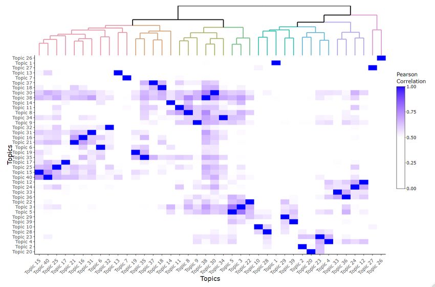
To get a better overview of climate change topics discussed in our corpus, we estimate
the correlated topic model (CTM) of Lafferty and Blei (2006) on our corpus. The CTM
model is an unsupervised generative machine-learning algorithm, which infers latent cor-
related topics among a collection of texts.16 In particular, each text is a mixture of K
topics, and each topic is a mixture of V words. The approach yields: (i) a vector of topic
attribution θk,n,t,s for each news article where K
P
k=1 θk,n,t,s = 1 with θk,n,t,s ≥ 0, and (ii) a
vector of word probabilities ωv,k for each topic, where Vv=1 ωv,k = 1 with ωv,k ≥ 0. We
P
estimate the model with K = 40 topics; more details are provided in Appendix A.
In Table 3, we report the ten words or collocations (i.e. common sequences of two
words) with the highest probability for each topic (i.e. the ten largest ωv,k for each topic
k). We also organize the topics into eight clusters that constitute more general themes
for ease of interpretation; see Appendix A for details. From these clusters, we see that
climate change discussions in the news media is spread across several themes, which we
label as: (i) “Financial and Regulation,” (ii) “Agreement and Summit,” (iii) “Societal
Impact,” (iv) “Research,” (v) “Disaster,” (vi) “Environmental Impact,” (vii) “Agricultural
Impact” and (viii) “Other.”
[Insert Table 3 about here.]
To better understand how much attention the media devotes to these topics over time,
we compute the number of monthly article equivalents for each topic. This quantity
measures the hypothetical number of news articles uniquely discussing a specific topic for
a given period. Formally, the number of article equivalents between dates t1 and t2 for
P 2 PS PNt,s
topic k is defined as tt=t1 s=1 n=1 θk,n,t,s . We then aggregate the number of article
equivalents by theme.
16
Hansen, McMahon, and Prat (2018), Larsen and Thorsrud (2017) and Larsen (2017) estimate latent
topics using the popular Latent Dirichlet Allocation (LDA) model of Blei, Ng, and Jordan (2003). The
LDA model, however, does not account for possible correlations between topics. We find that allowing
for non-zero correlation with the CTM model generates more coherent topics.
13In Figure 1, we display the monthly number of article equivalents for each theme from
January 2010 to June 2018. The most discussed themes (in decreasing order) are: “Finan-
cial and Regulation,”“Agreement and Summit,”“Societal Impact,”“Research,”“Disaster,”
“Environmental” and “Agricultural Impact.” We observe significant time variations in the
percentage of coverage devoted to each theme. For instance, the “Agreement and Summit”
theme tends to have a larger number of article equivalents during months where there are
notable conferences on climate change. Similarly, we observe an increase in the “Disaster”
theme in 2012 and 2017, which had very destructive wildfire seasons. The time variation
of newspapers’ coverage of themes implies that each topic captures different dimensions
of the climate change discussion.
[Insert Figure 1 about here.]
3.2. Media Climate Change Concerns index
We build the MCCC index following the methodology in Section 2. We compute the
source-specific standard deviation σs necessary to obtain the standardized source-specific
Media Climate Change Concerns with media articles from 2003 to 2009. Then, we aggre-
gate the resulting source-specific indices to obtain the MCCC index for 2010 to 2018. In
Figure 2, we display the daily evolution of the index from 2003 to 2018. Note that the
2003 to 2009 period is forward-looking and is not used in the main analysis, but is still of
interest for validating the index. We interpret the daily index as a proxy for changes in
climate change concerns. We also display a 30-day moving average of the index to help
identify trends and events.17
[Insert Figure 2 about here.]
First, we see that the index’s spikes correspond to climate change events, such as the
2012 Doha United Nations (UN) Climate Change Conference or the Paris Agreement. We
17
This moving average can be interpreted as a proxy for the level of climate change concerns. This
requires an assumption that climate change concerns only decrease because of the passage of time and
that news published more than 30 days in the past does not have any effect on current climate change
concerns.
14also note that climate change concerns, proxied by the moving average, exhibit phases of
low and high values. A first period of elevated concerns is observed following the 2007 UN
Security Council talks on climate change and lasts until the beginning of 2010, after the
Copenhagen UN Climate Change Conference. The second elevated period starts at the end
of 2012, near the UN Climate Change conference, and lasts until the Paris Agreement.
Later, we note a spike in concerns around the time of U.S. President Donald Trump’s
announcement that the U.S. will withdraw from the Paris Agreement. These observations
suggest that our index captures meaningful events that correlate with increases in climate
change concerns.18
To extract the unexpected component of the MCCC index, we use a first-order au-
toregressive model. Specifically, at time t, we estimate an AR(1) model with three years
of data up to time t − 1 and use the prediction error for UMCt .19
3.3. S&P 500 stock universe and its greenhouse gas emissions intensity
Our analyses require the identification of green and brown firms. We define green (brown)
firms as firms that create economic value while minimizing (not minimizing) damages
that contribute to climate change. To quantify these damages, we use the greenhouse gas
(GHG) emissions disclosed by firms. We retrieve these variables from the Asset4/Refinitiv
database. Similar to Ilhan, Sautner, and Vilkov (2020), we focus on S&P 500 firms because
surveys of greenhouse gas emissions typically target these firms.20
The greenhouse gas emissions variable is separated into three scopes defined by the
GHG Protocol Corporate Standard.21 Scope 1 emissions are direct emissions from owned
or controlled sources. Scope 2 emissions are indirect emissions from the generation of
purchased energy. Scope 3 emissions are all indirect emissions (not included in Scope 2)
18
As our index is bounded at zero by construction, it is more likely to better capture increases than
decreases in climate change concerns.
19
Results are similar if an expanded window is used instead of a rolling window of three years. Similar
results are also obtained using an ARMA(p,q) model with lags chosen with the Bayesian information
criterion (BIC).
20
Our results and conclusions are robust when considering S&P 1500 firms. However, beyond the S&P
500 universe, few firms disclose their greenhouse gas emissions.
21
See https://ghgprotocol.org/standards.
15that occur in a firm’s value chain. These are reported in tonnes of carbon dioxide (CO2)
equivalents. We focus on total GHG emissions, defined as the sum of the three emis-
sions scopes.22 To account for the economic value resulting from a firm’s GHG emissions,
we scale total GHG emissions by the firm’s annual revenue obtained from Compustat.
Whether a firm is classified as green or brown depends on its position within the distri-
bution of firms by their total tonnes of CO2-equivalent GHG emissions attributed to $1
million of revenue at a point in time. This scaled-GHG variable is referred to as GHG
emissions intensity (see Drempetic, Klein, and Zwergel, 2020; Ilhan, Sautner, and Vilkov,
2020).23
In Table 4, we report the percentage of firms in the S&P 500 with available GHG
emissions (Panel A) and summary statistics for GHG emissions intensity (Panel B). While
our GHG emissions source differs from Ilhan, Sautner, and Vilkov (2020), who use the
Carbon Disclosure Project database24 , we see that our coverage of S&P 500 firms is similar,
averaging slightly above 50% of the firms in the universe. The average emissions intensity
is 682.49 tonnes of CO2-equivalent emissions per $1 million in revenue. The 25th and 75th
percentiles are 21.54 and 378.93, respectively. The quartiles, together with the skewness
and kurtosis statistics, indicate a distribution of GHG emissions intensity that is highly
positively skewed and fat-tailed.
[Insert Table 4 about here.]
Finally, we note that GHG emissions are typically reported with a one-year delay.
Similar to Ilhan, Sautner, and Vilkov (2020), we account for this by shifting the GHG
emissions intensity variable by 12 months in our analyses.
22
The results from our analysis are similar when excluding Scope 3 emissions.
23
The environmental dimension of ESG scoring is an alternative variable to classify firms on the green
to brown spectrum. However, Drempetic, Klein, and Zwergel (2020) suggest that these scores do not
adequately reflect firms’ sustainability. Additionally, Berg, Koelbel, and Rigobon (2019) show that the
correlations between ESG scores of different data providers are weak, indicating a lack of reliable and
consistent scoring methodology across providers.
24
See https://www.cdp.net/.
164. Empirical results on the performance of green vs. brown stocks
We first construct portfolios of green and brown stocks and test whether the green portfolio
outperforms the brown portfolio when there are unexpected increases in climate change
concerns, both using a conditional mean analysis (Section 4.1) and a multivariate factor
analysis (Section 4.2). Next, we analyze the impact of climate change concerns in the
cross-section of stock returns (Section 4.3). In particular, we evaluate whether industry-
relative GHG emissions intensity matters, and whether firms that do not disclose their
emissions are impacted by unexpected changes in climate change concerns.
4.1. Conditional mean analysis
We divide assets into three groups: green, neutral and brown. Green (brown) stocks are
firms with a GHG emissions intensity variable in the lowest (highest) quartile of all firms’
values on day t. Neutral firms are the remainder of firms that disclose GHG emissions
data. We then build, for each day, equal-weighted portfolios for these groups.25
Our first analysis focuses on the average return of the green minus brown (GMB) port-
folio conditional on the UMC variable. In Figure 3, we display the average performance of
the GMB portfolio conditional on threshold values for UMC, obtained as the percentiles
of UMC over the 2010-2018 period. We see a clear positive relationship between the av-
erage return and UMC. In particular, when UMC is above its median, we notice strong
increases in the GMB portfolio average return as the thresholds becomes larger, especially
at the extreme. Moreover, the average GMB portfolio return is always higher when the
UMC is above the threshold than when it is below. These preliminary findings indicate
that green firms outperform brown firms when there are unexpected increases in climate
change concerns.
[Insert Figure 3 about here.]
25
While GHG emission is updated yearly, stocks can enter or exit the S&P500 universe at any day.
Also, we note that results are qualitatively similar if market capitalization-weighted portfolios are used
instead.
174.2. Multivariate factor analysis
We now consider a multivariate linear regression framework to control for other factors
that potentially drive stock returns. We regress the green minus brown (p = GM B), green
(p = G), brown (p = B), and neutral (p = N ) portfolios’ excess returns, rp,t , on UMCt ,
and common factors used in the financial literature (ft ). We consider the five Fama-French
factors (Fama and French, 2015): (i) MKT, the excess market return; (ii) SMB, the small
minus big factor; (iii) HML, the high minus low factor; (iv) RMW, the robust minus
weak factor; and (v) CMA, the conservative minus aggressive factor. We also include (vi)
MOM, the momentum factor of Carhart (1997).26 This yields the following specification:
rp,t = cp + βUMC
p UMCt + βp ft + εp,t , (7)
where cp is a constant, βpUMC and βp are regression coefficients, and εp,t is an error term.
Given the Pastor, Stambaugh, and Taylor (2020) model, we expect that βUMC
G > 0, βUMC
B <
0 and βUMC UMC
GMB > 0. We expect βN to be positive or not significantly different from zero.
The latter case implies that investors switch from browner firms to greener firms when
there is an unexpected increase in climate change concerns. However, the former case
implies that investors disinvest from brown firms and reinvest in the rest of the market.
This pattern is consistent with a brown firms screening mechanism, which, as reported
in Bolton and Kacperczyk (2020), tends to be the preferred strategy for institutional
investors.
Estimation results are reported in Table 5. First, let us consider the GMB portfolio.
We see that the estimated coefficient for UMC aligns with our hypothesis. Specifically, a
one-unit increase in UMC implies an additional daily positive return of 9 basis points. This
effect is highly significant, with the t-stat at about 3.3 — above the significance hurdle of
3.0 proposed by Harvey, Liu, and Zhu (2016). The estimated coefficients indicate that the
GMB portfolio is positively related to MKT, HML, SMB and MOM, and negatively related
to CMA and RMW. Thus, the GMB portfolio emphasizes small firms with lower growth,
26
Factors and risk-free rate data are retrieved from Kenneth French’s website at http://mba.tuck.
dartmouth.edu/pages/faculty/ken.french/index.html.
18aggressive investment policies and weak operating profits. The CMA coefficient (-0.559)
is large compared to the other coefficients. This finding is consistent with green firms
investing more and brown firms investing less, which is another implication of the Pastor,
Stambaugh, and Taylor (2020) model. This prediction arises from the idea that green
firms’ capital costs are lower than brown firms’. Thus, more investment opportunities
for green firms have a positive net present value, resulting in a higher investment level
relative to their size than for brown firms.
[Insert Table 5 about here.]
Looking at the green portfolio, we find a positive and highly significant exposure to
UMC. For the brown portfolio, we find a highly significant negative coefficient. Moreover,
we find that the UMC coefficient for the brown portfolio is larger in absolute value than
for the green portfolio (0.054 vs. 0.037). We also find that neutral firms have a positive
relationship with unexpected changes in climate change concerns. However, the coefficient
for the neutral portfolio is lower than for the green portfolio (0.022 vs. 0.037). This finding
implies that investors’ strategies regarding climate change tend toward a screening of
brown firms, with reallocation to both green and neutral firms, consistent with Bolton
and Kacperczyk (2020).
4.3. Climate change concerns in the cross-section of stock returns
In the previous section, we showed that the stock returns of a portfolio of firms with low
(high) GHG emissions intensity are positively (negatively) associated with unexpected
changes in climate change concerns. We now test whether we can recover this relationship
using stock-level return exposures to UMC. Moreover, we test whether the results still
hold when we consider variations in GHG emission intensity within industries, rather than
across industries. We also analyze whether firms that do not disclose their GHG emissions
are affected by climate change concerns based on their industry, and if this effect differs
from firms that disclose their emissions.
194.3.1. General model
We first define lGHGi,t as the cross-sectionally standardized logarithm of the greenhouse
gas intensity of firm i available at time t.27 The standardization is performed by focus-
ing on the cross-sectional variation across firms. We then estimate the following panel
regression model:
ri,t = c + γlGHG lGHGi,t + γUMC+ γUMC
lGHG
lGHGi,t UMCt + βi ft + i,t , (8)
where ri,t is the excess stock return of firm i at time t, and ft are control factors. We
consider one-factor (MKT), three-factor (MKT, HML, SMB) and six-factor (MKT, HML,
SMB, RMW, CMA, MOM) specifications. Coefficients γ • are common to all firms, while
βi are firm-specific coefficients.28
In specification (8), the exposure of firms to the unexpected changes in climate change
concerns is γUMC + γUMC
lGHG
lGHGi,t , including a common component and one that depends
on a firm’s level of log-GHG emissions intensity relative to other firms. Given our previous
results for the neutral portfolio, we expect a positive value for the common component,
γUMC . We also expect a significant negative value for γUMC
lGHG
, so that the higher (lower) a
firm’s level of GHG emissions intensity, the more negative (positive) the firm’s exposure is
to unexpected increases in climate change concerns, in line with the prediction by Pastor,
Stambaugh, and Taylor (2020).29
We also consider an asymmetric specification to test our earlier finding that brown
firms appear to be more affected (in absolute terms) by unexpected changes in climate
change concerns than green firms. To do so, we introduce the variable Bi,t , which is equal
to one when lGHGi,t > 0; that is, an indicator variable that is equal to one when the
27
Similar results are obtained if we use the cross-sectional median for standardization as opposed to
the cross-sectional average.
28
In addition, we consider a firm fixed-effects specification where c is replaced by ci as well as a threshold
model in which regression parameters are conditioned on the value of UMC being above or below a certain
threshold calibrated with the Bayesian information criterion. Our conclusions remained unchanged.
29
A Fama-MacBeth cross-sectional regression analysis was also performed and provided similar results
(see Appendix B).
20log-GHG emissions intensity of firm i is above the cross-sectional average at time t. We
then estimate the following panel regression model, which nests the previous one:
ri,t = c + γlGHG + γlGHG
B
Bi,t lGHGi,t
+ γUMC + γUMC UMC
lGHG
lGHGi,t + γlGHG-B
lGHGi,t Bi,t UMCt + βi ft + i,t . (9)
In this specification, the exposure of firms to unexpected changes in climate change con-
cerns is γUMC + γUMC UMC
lGHG
lGHG i,t + γlGHG-B
lGHGi,t Bi,t . We expect a negative coefficient for
γUMC
lGHG-B
, which would imply that browner firms (i.e. below the cross-sectional average) are
more exposed in absolute terms to unexpected changes in climate change concerns than
greener firms (i.e. above the cross-sectional average).
Our panel regression models allow us to test the implication of the model by Pastor,
Stambaugh, and Taylor (2020); that is, green firms outperform brown firms when there
are unexpected increases in climate change concerns. Our asymmetric specification allows
us to test the implication of Bolton and Kacperczyk (2020); that is, institutional investors
tend to screen for emissions-intense firms, which are clustered in a few salient industries,
but do not necessarily prioritize investing in the greenest firms. This observation implies
an asymmetry between greener and browner firms’ exposures and a positive relationship
between neutral firms and UMC, as observed in our portfolio analysis.
Panel regression results are reported in Table 6. For all specifications, we find γUMC
lGHG
to be negative and highly significant, consistent with our expectations. The one-factor
model’s coefficients imply that firms with a one standard deviation log-GHG emissions
intensity above the cross-sectional mean have a negative exposure to unexpected changes
in climate change concerns of about -0.024 (i.e. the sum of the coefficients of UMC and
UMC × lGHG) in the non-asymmetric specification. We note that only the coefficient of
the interaction between U M C and lGHG is significant across all three non-asymmetric
specifications using different sets of controls. For the asymmetric specifications, firms with
a one standard deviation log-GHG emissions intensity above the cross-sectional mean have
an exposure of -0.045, and firms with a one standard deviation log-GHG emissions inten-
21sity below the cross-sectional mean have an exposure of 0.032. Results are similar for the
other asymmetric specifications. We note that the common factor UMC, the interaction
UMC × lGHG and the asymmetric term UMC × lGHG × B are all significant across all
of the three sets of factors. Overall, the results are in line with Pastor, Stambaugh, and
Taylor (2020), Bolton and Kacperczyk (2020) and the results of our portfolio analysis.
[Insert Table 6 about here.]
4.3.2. Within-industry analysis
As noted by Ilhan, Sautner, and Vilkov (2020), most of the variation in GHG emissions
intensity across firms can be attributed to industries. Bolton and Kacperczyk (2020)
also find that institutional investors implement exclusionary screening based on direct
emissions intensity in a few industries. We now test whether investors also consider the
variation in GHG emissions intensity within industries when there are unexpected changes
in climate change concerns. To do so, we re-estimate our panel regression models in (8)
and (9), but now define lGHGi,t as the daily within-industry cross-sectionally standardized
GHG emissions intensity of firm i at time t. The firms are grouped using the Fama-French
48 industry classification.30
Estimation results are reported in Table 7. As in our previous analyses, we find that
the greener (browner) the firms are within an industry, the more positive (negative) their
stock price’s response is to unexpected changes in climate change concerns. However, we
do not observe an asymmetry between firms that are above or below the within-industry
average GHG emission intensity. This result is expected, as Bolton and Kacperczyk (2020)
suggest that institutional investors tend to screen firms on direct emissions intensity in
a few salient industries. Thus, the asymmetry is only observed when comparing GHG
emissions intensity across industries, not within industries. Moreover, the size and sig-
nificance of coefficients is notably smaller than when we do not consider industry-specific
30
Industry data were retrieved from Kenneth French’s website at http://mba.tuck.dartmouth.edu/
pages/faculty/ken.french/index.html. We obtain similar results using a one- or two-digit SIC indus-
try definition.
22greenness and standardize across all firms in our universe. While investors consider emis-
sions intensity within industries, they put more emphasis on how firms compare to other
firms generally, not necessarily to firms within their industry.
[Insert Table 7 about here.]
4.3.3. Firms that do not disclose GHG emissions
Investors may classify firms that do not disclose their GHG emissions as green or brown
using information about the firm’s industry. As noted in Ilhan, Sautner, and Vilkov
(2020), close to 90% of the variation in GHG emissions across firms is explained by
industry. Moreover, Matsumura, Prakash, and Vera-Muñoz (2014) find that firms that
do not disclose their GHG emissions get penalized relative to firms that disclose. We now
analyze whether firms that do not disclose their GHG emissions are affected by climate
change concerns based on their industry, and if this effect differs from those that disclose
their emissions. To do so, for each day t, we set the GHG emissions intensity of non-
disclosing firms equal to the average for their industry. We then estimate the following
model:
ri,t = c + γlGHG+ γlGHG lGHG lGHG
B
Bi,t + γ UD
UD i,t + γ B-UD
B i,t UD i,t lGHGi,t
+ γUMC + γUMC UMC UMC UMC
lGHG
+ γ lGHG-B
B i,t + γ lGHG-UD
UD i,t + γ lGHG-B-UD
Bi,t UDi,t lGHGi,t UMCt
+ βi ft + i,t , (10)
where lGHGi,t is defined as the industry average GHG emissions intensity for firms that
do not disclose, and UDi,t is equal to one if the GHG emissions intensity of firm i at time
t is not disclosed.
Estimation results are reported in Table 8. First, we see that our main results are
unchanged. The lower (higher) a firm’s log-GHG emissions intensity is relative to other
firms, the more positive (negative) the firm’s exposure is to unexpected changes in climate
change concerns. The asymmetric relationship remains: Brown firms (below the cross-
sectional average) are more exposed in absolute value than green firms (above the cross-
sectional average). Interestingly, we find this is also the case for firms that do not disclose
23their GHG emissions, suggesting that industry information is also used to establish a
firm’s greenness.
[Insert Table 8 about here.]
5. Dimensions of climate change concerns
So far, we have established a relationship between unexpected changes in climate change
concerns, proxied by the MCCC index and the UMC variable, and returns of green vs.
brown firms. However, climate change is a broad subject with many facets, such as
disasters, financial impacts, environmental impacts and regulatory impacts. Engle et al.
(2020) suggest analyzing whether news about physical damages from climate change and
news about regulatory risks have different impacts on stock returns. Moreover, the model
of Pastor, Stambaugh, and Taylor (2020) implies that the effect of climate change concerns
arises from two channels: (i) changes to expected cash flow and (ii) changes to investor
tastes. Below, we build topical indices of Media Climate Change Concerns and analyze
which dimensions drive the relationship between unexpected increases in climate change
concerns and stock returns for green and brown firms. We then try to attribute these
subjects to cash flow and/or taste channels.
To build the topical MCCC indices, we consider a topic-attribution weighted version
of (3):
Nt,s
X
concernsk,t,s = θk,n,t,s concernsn,t,s , (11)
n=1
where θk,n,t,s is obtained from the estimated CTM (see Section 3.1 and Appendix A).
We normalize and aggregate the scores for each index, following the steps of Section 2.3.
This yields K = 40 topical MCCC indices.31 We then estimate topical unexpected change
in climate change concerns, which we denote by UMCk,t , using the procedure outlined in
Section 2.4 and Section 3.2. Please refer to Table 3 for the list of topics/themes.
31
The MCCC index is obtained as a special case of (11) by setting θk,n,t,s = 1 ∀ n, t, s.
24To identify which themes and topics drive the relationship between climate change
concerns and stock returns, we reconsider the approach of Section 4.2 with the following
specification:
rp,t = cp + βUMC
p
k
UMCk,t + βp ft + p,t . (12)
The quantity of interest is now βUMC
p
k
rather than βUMC
p .32
Regression results are reported in Table 9. We find that for all topics, the sign of the
relationship is in line with our hypothesis: positive for the GMB and green portfolios, and
negative for the brown portfolio. However, only for 24 out of the 40 topics, the estimated
coefficient is significant at the 5% confidence level. Specifically, we find that the return
is most influenced by news articles expression climate change concern about X and Y
(topics).
Pastor, Stambaugh, and Taylor (2020) note that the price impact can happen through
two mechanisms: explain. From the topic analysis, we can confirm that both channels
play a role. ....
[Insert Table 9 about here.]
Summarizing the results by theme, we find that “Financial and Regulation,” “Agree-
ment and Summit,”“Societal Impact,”“Research,” and “Disaster” contain multiple topics
with significant coefficients. Given the financial nature of the topics in “Financial and
Regulation,” we posit this theme primarily affects the cash flow channel. “Research”,
however, is likely to only affect the tastes channel, as research results hardly impact firms’
cash flows, at least in the short-term. The “Agreement and Summit” theme is likely to
affect both channels. On the one hand, regulations can have direct impacts on firms’
future cash flows. On the other hand, the discussions taking place at these conferences
often underline the future disastrous consequences of climate change, which can affect
investors’ tastes. We posit that the “Societal Impact” theme is likely to affect the tastes
32
The analysis based on the panel specification presented in Section 4.3 yields the same conclusion
as (12).
25You can also read