Clouds LMDz Training - December 2021 J-B Madeleine and the LMDz team - For more detail, see Madeleine et al. 2020
←
→
Page content transcription
If your browser does not render page correctly, please read the page content below
Clouds
 LMDz Training – December 2021
J-B Madeleine and the LMDz team

For more detail, see Madeleine et al. 2020
 https://doi.org/10.1029/2020MS002046

                                             1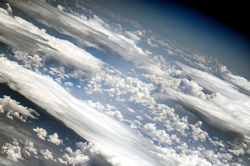
Picture by Oleg Artemyev taken from the ISS 2
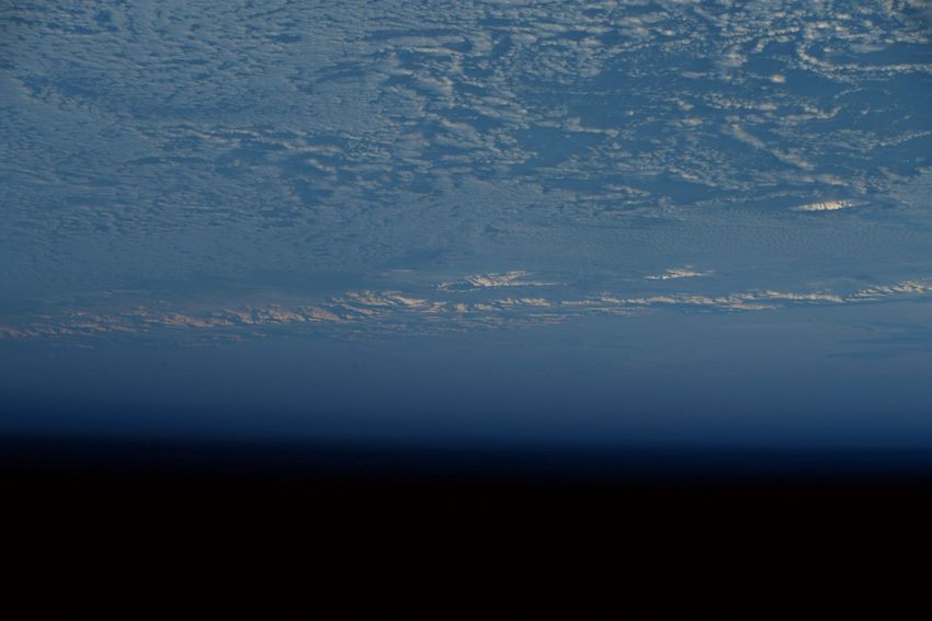
Picture by Thomas Pesquet taken from the ISS 3
Radiative forcing
        LW radiative forcing

       Positive : clouds reduce
       the LW outgoing radiation

       Annual mean : +29 W m-2

         SW radiative forcing

       Negative : clouds reflect
       the incoming SW radiation

       Annual mean : -47 W m-2

          Net forcing : Cooling

        Annual mean : -18 W m-2

« The single largest uncertainty in
determining the climate sensitivity to either
natural or anthropogenic changes are
  clouds and their effects on radiation »       4
              5th IPCC report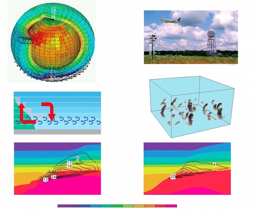
Visualize clouds in LMDZ
prw (2D) : Precipitable water (kg/m2)
pluc/plul (2D) : Convective/lsc rainfall (kg/m2/s)
snow (2D) = surface snowfall (kg/m2/s)
lwp (2D) : Cloud liquid water path (kg/m2)
iwp (2D) : Cloud ice water path (kg/m2)

ovap (3D) : water vapor content (kg/kg)
oliq (3D) : cloud liquid water content (kg/kg)
ocond (3D) : cloud liq+ice water content (kg/kg)

pr_lsc_l (3D) : lsc rain mass fluxes (kg/m2/s)
pr_lsc_i (3D) : lsc snow mass fluxes (kg/m2/s)

rneb (3D) : cloud fraction (%)
cldh (2D) : High-level cloud cover (%)
cldm (2D) : Mid-level cloud cover (%)
cldl (2D) : Low-level cloud cover (%)
cldt (2D) : Total cloud cover (%)

low‐level clouds = below 680 hPa or ∼3 kmlevel clouds = below 680 hPa or ∼3 km3 km
mid‐level clouds = below 680 hPa or ∼3 kmlevel clouds = between 680 and 440 hPa         5
high‐level clouds = below 680 hPa or ∼3 kmlevel clouds = above 440 hPa or ∼3 km6.5 km
Modeling clouds : a challenge
Microphysics                                        Macrophysics

                               Spatial scale ~ µm               Spatial scale ~ km
                                Time scale ~ 1 s               Time scale ~ 15 min

                                                                                     6
[Libbrecht, 2005]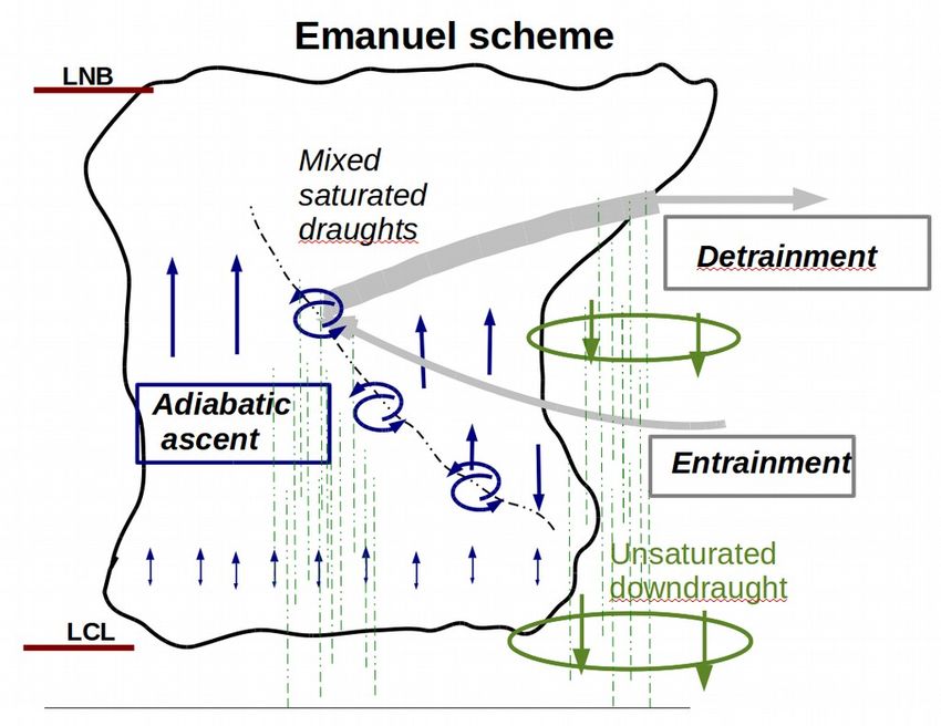
Fundamental process
●
    Clausius-Clapeyron equation :

●
    Saturation mass mixing ratio :

                                 , where esat(T) grows exponentially with temperature

●
    Clouds form when an air parcel is cooled :
                    qc = qt - qsat(Tf,p)

                                                        q
                    qsat(Tf,p)    qt       qsat(Ti,p)

●
    But clouds do not look like that :
                                                                          Comet, UCAR
                                                                                        7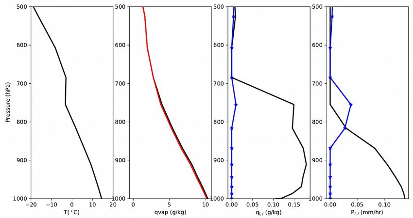
Many processes in one grid cell

                            Around 8 hours of simulation by a Cloud Resolving Model (CRM) – C. Muller, LMD
        Thermals in a
        Large-Eddy Simulation (LES)
                                           Conditional sampling
                                           of thermals based
                                           on a tracer emitted
                                           at the surface.
z (m)

                                                                                                             8
                                                                     Lemone et Pennell, MWR, 1976
                                   Couvreux et al., BLM, 2010
                    X (m)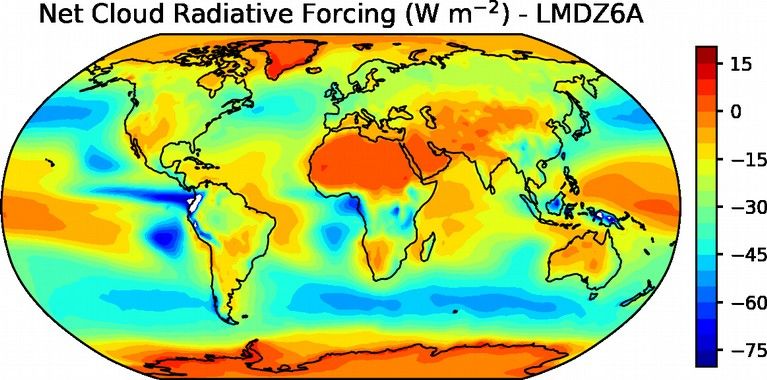
Statistical cloud scheme
        « all or nothing » model :
        If q > qsat 100% cloudy, otherwise clear sky.

        « statistical » model : statistical distribution of q' around q

                                                              Saturation deficit

                                                                           9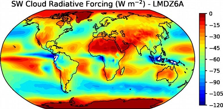
Statistical cloud scheme 2/2
                                    Mean total water content :

                                    Domain-averaged condensed water content :

                                    Cloud fraction :

 The goal of a cloud scheme is       In-cloud condensed water content :
therefore to compute qcin and the
  cloud fraction based on the
        different physical
       parameterizations.                                                       10
Architecture of the cloud scheme
CAREFUL : clouds are
evaporated/sublimated at the beginning of
each time step (~15 min), but vapor, droplets
and crystals are prognostic variables. In other
words, clouds can move but can't last for
more than one timestep (meaning that for
example, crystals can't grow over multiple
timesteps).
111. Deep convection
qcin is computed by the deep
convection scheme and is
12
known → cloud fraction is found2. Shallow convection 1/2
132. Shallow convection 2/2
[Jam & al., BLM, 2013]
Bi-Gaussian distribution of saturation deficit s:
One mode for thermals : sth, σth
One mode for their environment : senv, σenv
Senv, sth, and α are given by the shallow convection
scheme, and the distribution’s variances are
parameterized following :
[Jam & al., BLM, 2013]
qcin and the cloud fraction can be
computed following :
148m gridcell
Fo
rc
in
g
Field campaign
Detailed simulation
(LES : Large Eddy Simulation)
The 1D cloud fraction is 12km
computed using the set
of parameterizations
Altitude (km)
Altitude (km)
The fraction of
the LES domain
covered by clouds
is computed at
Evaluation each time step
and for each level,
resulting in a 1D
cloud fraction
Local solar time Local solar time3. Large scale condensation
Temperature, water vapor, clouds and precipitation over one timestep
1 REEVAPORATION 2 CLOUD FORMATION 3 PRECIPITATION 163. Large scale condensation
●
Rain/snow is partly evaporated in the grid below (parameter
controlling the evaporation rate) :
1 REEVAPORATION
If there is shallow qcin and the cloud fraction can be
2 CLOUD FORMATION convection computed following :
If there is no
shallow
convection
qcin and the cloud fraction can be In both cases, cloud
computed following : phase is parameterized
using a simple function
of temperature :
Log-normal distribution of total water qt
using a prescribed variance
173. Large scale condensation
3 PRECIPITATION
●
A fraction of the condensate falls as rain (parameters controlling the maximum water
content of clouds and the auto-conversion rate) :
●
Another fraction is converted to snow following :
●
This fraction depends on the same temperature function
as clouds → rain can be created below freezing
●
When this occurs, the resulting liquid precipitation
is converted to ice.
●
When freezing, rain releases latent heat, which can
potentially bring the temperature back to above freezing.
If this is the case, a small amount of rain remains liquid to
stay below freezing.
Growth of an ice crystal at the expense
of surrounding supercooled water drops 18
[Wallace, 2005]Tuning parameters
coef_eva=0.0001
cld_lc_lsc=0.00065
cld_tau_lsc=900
ffallv_lsc=0.8
ratqsp0=45000
ratqsdp=10000
ratqsbas=0.002
ratqshaut=0.4
19Radiative transfer
Radiative transfer equation :
Solving the radiative transfer equation requires :
● q to compute the optical depth ;
rad
●
Cloud droplet and crystal sizes to compute the optical properties ;
●
The cloud fraction α to compute the heating rates in the clear-sky (1-
α) and cloudy (α) columns.
20Optical properties of liquid clouds
(see O. Boucher's talk)
Link cloud droplet number concentration to soluble
aerosol mass concentration (Boucher and Lohmann, Tellus, 1995)
= CDNC
Size-dependent computation of cloud
optical properties (Fouquart [1988] in the
SW, Smith and Shi [1992] in the LW)
21Optical properties of ice clouds
Optical properties are computed using
Ebert and Curry [1992], based on the
computed crystal sizes.
[Ebert, 1992]
Crystal sizes follow
r = 0.71T + 61.29 in μm
[Iacobellis et Somerville 2000]
with rmin ~ 10 μm (tuneable)
for T < -81.4°C [Heymsfield et
al. 1986]
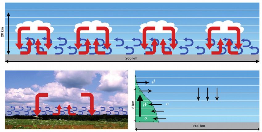
22CF versus height is known, but radiation also
needs to know the total cloud cover ; we
therefore parameterize the cloud overlap
20 km
q < qsat
200 km For the GCM, these two scenes
are identical ;
20 km
200 km
er !
l d be bett Used in LMDz
Wou
High cover Intermediate cover Low cover
23
[Radiation parameterization and clouds, Hogan, 2009]Subgrid scale heterogeneity
and 3D effects : ecRad ( )
Monte-Carlo Independent Column Approx.
(McICA, Pincus et al. 2005)
●
Takes into account cloud sizes but also
horizontal radiative transfer in the case
of SPARTACUS
●
Cloud sizes must be parameterized
along with cloud fraction and opacity
SPARTACUS (Hogan et al., 2016)
Accounts for 3D effects 24
© figures by Robin Hogan, ECMWFWelcome to the LMDz team ! 25
Importance of cloud phase

●
    Clouds reflect sunlight (negative
    forcing, cooling) and emit in the
    infrared (positive forcing,
    warming) ;
●
    For the same water content, liquid
    clouds reflect more sunlight than
    ice clouds ;
●
    For liquid clouds : if the cloud water
    content increases, there is a
    negative forcing (reflection
    dominates) ;
●
    For ice clouds : if the cloud water
    content increases, the forcing
    depends on the size of the crystals.

                                              [Liou 2002]
                                                            26
Précision sur les sorties
●
L'eau nuageuse que voit le rayonnement n'est pas la même que
l'eau nuageuse utilisée dans la physique et la dynamique. Lors de
la conversion en précipitation dans fisrtilp, c'est une moyenne de
l'eau restante dans le nuage PENDANT la précipitation qui est
stockée dans radliq pour le rayonnement, et non l'eau restante À
LA FIN du pas de temps, qui elle est utilisée dans la physique et
advectée par la dynamique. (C'est un choix qui peut être discuté.)
Du coup, il est facile de se perdre et de voir des incohérences
dans les sorties entre l'eau qui sort du rayonnement et celle qui
sort de la physique.
●
Pour résumer, sont écrites ci-dessous les variables qui sont égales
avec entre parenthèses le nom de la routine correspondante ou
"netcdf" quand il s'agit des sorties :
●
Rayonnement : xflwc(newmicro) + xfiwc(newmicro) = cldliq(physiq)
= radliq(fisrt) = lwcon(netcdf) + iwcon(netcdf)
●
Physique / dynamique : ql_seri(physiq) + qs_seri(physiq) =
ocond(netcdf)
●
Attention cependant : radliq(fisrt) /= ocond(netcdf) autrement dit :
lwcon(netcdf) + iwcon(netcdf) /= ocond(netcdf) (ce qui n'est pas du
tout évident)
●
Si on enlève la moyenne faite par fisrtilp lors de la conversion en
précipitation, on obtient bien l'égalité entre l'ensemble des
variables. Ci-contre un exemple de profils des différentes
variables. Cette moyenne tend à augmenter l'eau nuageuse
transmise au rayonnement. Comme il s'agit d'une moyenne sur le
pas de temps plutôt qu'une eau restante à la fin du pas de temps,
elle tend donc, a priori, à faire des nuages plus brillants. Cette
moyenne remonte à Le Treut et Li (1991), où le pas de temps
physique du modèle était d'une demi-heure contre 15 min 27
actuellement.You can also read