CNN and Deep Sets for End-to-End Whole Slide Image Representation Learning
←
→
Page content transcription
If your browser does not render page correctly, please read the page content below
Proceedings of Machine Learning Research 143:301–311, 2021                  MIDL 2021 – Full paper track

      CNN and Deep Sets for End-to-End Whole Slide Image
                  Representation Learning

Sobhan Hemati1 , Shivam Kalra1 , Cameron Meaney 2 , Morteza Babaie 1 , Ali
Ghodsi 4,5 , H.R. Tizhoosh 1,5
1
    Kimia Lab, University of Waterloo, Waterloo, ON, Canada
2
    Department of Applied Mathematics, University of Waterloo, Waterloo, ON, Canada
4
    Data Analytics Laboratory, University of Waterloo, Waterloo, ON, Canada
5
    Vector Institute, MaRS Centre, Toronto, ON, Canada

                                                Abstract
      Digital pathology has enabled us to capture, store and analyze scanned biopsy samples as
      digital images. Recent advances in deep learning are contributing to computational pathol-
      ogy to improve diagnosis and treatment. However, considering challenges inherent to whole
      slide images (WSIs), it is not easy to employ deep learning in digital pathology. More im-
      portantly, computational bottlenecks induced by the gigapixel WSIs make it difficult to
      use deep learning for end-to-end image representation. To mitigate this challenge, many
      patch-based approaches have been proposed. Although patching WSIs enables us to use
      deep learning, we end up with a bag of patches or set representation which makes down-
      stream tasks non-trivial. More importantly, considering set representation per WSI, it is
      not clear how one can obtain similarity between two WSIs (sets) for tasks like image search
      matching. To address this challenge, we propose a neural network based on Convolutions
      Neural Network (CNN) and Deep Sets to learn one permutation invariant vector represen-
      tation per WSI in an end-to-end manner. Considering available labels at the WSI level -
      namely, primary site and cancer subtypes - we train the proposed network in a multi-label
      setting to encode both primary site and diagnosis. Having in mind that every primary site
      has its own specific cancer subtypes, we propose to use the predicted label for the primary
      site to recognize the cancer subtype. The proposed architecture is used for transfer learning
      of WSIs and validated two different tasks, i.e., search and classification. The results show
      that the proposed architecture can be used to obtain WSI representations that achieve
      better performance both in terms of retrieval performance and search time against Yot-
      tixel, a recently developed search engine for pathology images. Further, the model achieved
      competitive performance against the state-of-art in lung cancer classification.
      Keywords: Whole-Slide Image Representation Learning, Whole-Slide Image Search, Multi-
      Instance Learning, Multi-label Classification, Digital Pathology

1. Introduction
The advent of digital pathology has provided researchers with a wealth of scanned biopsy
samples. Accordingly, the amount of data stored in digital pathology archives has grown sig-
nificantly as entire specimen slides or whole slide images (WSIs) can be imaged at once and
stored as an digital images. The increased acquisition of this type of data has opened new
avenues in the quantitative analysis of tissue histopathology, e.g., support the diagnostic
process by reducing the inter- and intra-observer variability among pathologists. Consider-

© 2021 S. Hemati, S. Kalra, C.M. , M.B. , A.G. & H. Tizhoosh.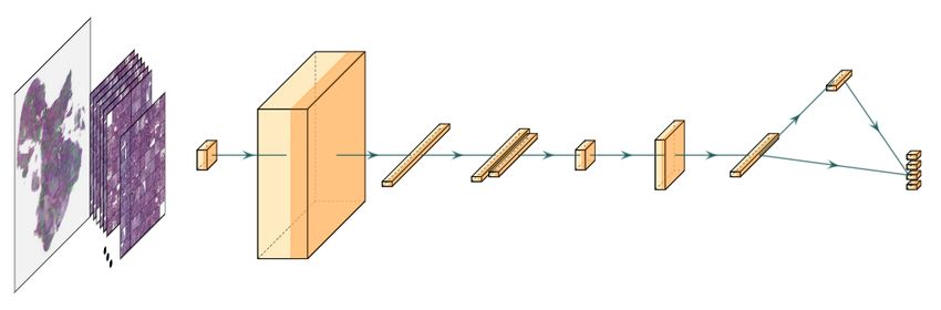
Hemati Kalra       Tizhoosh

ing this, as well as other advantages of digital pathology (Niazi et al., 2019), one expects
that histopathology images can be analyzed using the myriad computer vision algorithms
currently available for similar tasks. As such, the usage of deep learning for WSI analysis
has become an active area of research. Unfortunately, scientific progress with these data
has been slowed because of difficulties with the data itself. These difficulties include highly
complex textures of different tissue types, color variations caused by different stainings,
rotationally invariant nature of WSIs, lack of labelled data and most notably, and the ex-
tremely large size of the images (often larger than 50,000 by 50,000 pixels). Additionally,
these images are multi-resolution; each WSI may contain images from different zooming
levels, primarily 5x, 10x, 20x, and 40x magnification (Tizhoosh and Pantanowitz, 2018).
    The largest obstacle hindering the application of deep networks in computational pathol-
ogy tasks is the sheer size of the images that makes it infeasible - or perhaps even impossible
- to obtain a vector representation for a given WSI. In practice, this hurdle is often bypassed
by simply considering small ’patches’ of the WSI, a set of which is meant to represent the
entire WSI (Faust et al., 2018; Chenni et al., 2019). Existing patching schemes allow us
to split the WSI into tiles to be inputted to deep CNNs for WSI representation learning.
However, such representations impose some new challenges. Firstly, significant memory re-
sources are necessary to store sets of high dimensional vector representations for each WSI.
Secondly, and more challenging, employing set representations for downstream problems,
e.g., WSI classification and retrieval is not straightforward.

2. Related work
Considering gigapixel nature of WSIs, there is a large body of work on producing WSI
representations suitable for different quantitative tasks. Authors in (Coudray et al., 2018)
trained an Inception-V3 model on patches extracted from 20x and 5x magnifications for lung
cancer subtype classification. To predict a label for a WSI from patch label predictions,
they employed a simple heuristic based on the proportion of the patches assigned to each
category. Hou et al. (Hou et al., 2016) proposed a patch-level classifier for WSI classification.
In order to combine their patch-level predictions, they proposed a decision fusion model.
By considering the spatial relationships between the patches, they utilized an expectation-
maximization method to obtain the set of distinct patches from each WSI. Tellez et al.
(Tellez et al., 2019) proposed a two-step method to employ CNNs for WSI classification. To
this end, in the first stage they compress image patches using unsupervised learning. Then
compressed patches are placed together (such that their spatial position is kept) and they
are fed to another CNN for final prediction.
    These and many other papers all used patch level training with decision fusion methods
to achieve WSI level labels. Although this can be a helpful approach for classification, for
many other tasks like search, it leads to a set of vector representations which have to be used
to calculate distances between WSIs. There is no established way how to calculate distance
between two sets of vectors. For example, authors in (Kalra et al., 2020b; Riasatian et al.,
2021) resorted to the heuristic approach of taking the median of minimums to calculate the
total distance between two WSIs. Although they were able to show that their approach
achieved satisfactory performance, due to the computational complexity inherent to the
median of minimums method, the retrieval time can be considerably high unless binary

                                              302
CNN and Deep Sets for End-to-End Whole Slide Image Representation Learning
encoding algorithms (Hemati et al., 2020) are used. On the other hand, representing a WSI
using one vector not only removes the necessity of resorting to decision fusion methods in
classification, but also considerably simplifies the WSI search problem.
In the context of WSI representation learning, different methods have been proposed to
obtain one vector for representation of each WSI. For example, in Spatio-Net (Kong et al.,
2017) patches are first processed by a CNN, then the embedded patches with each neighbor
are fed into 2D-LSTM layers to capture the spatial information. Representing each WSI
as bag of image patches makes multiple instance learning schemes (MIL) (Dietterich et al.,
1997; Kalra et al., 2020a; Campanella et al., 2018) a natural approach to WSI representation
(Quellec et al., 2017). More precisely, the mentioned patch-based CNN by Hou et al. (Hou
et al., 2016) can be seen as a MIL method to determine instance classes. However, the
two-stage neural networks and EM approach appeared to perform sub-optimally. Another
recent work on MIL is attention -based MIL (Ilse et al., 2018) which was shown to be
effective on medical data. Considering this, employing permutation invariant networks show
potential as an effective approach for developing end-to-end WSI representation learning.
One recent work on permutation invariant networks is Deep Sets (Zaheer et al., 2017). In the
original work detailing Deep Sets, the authors specified a permutation-invariant function
and proposed to employ universal set function approximators in neural network. They
showed that despite its simplicity, their proposed permutation-invariant architecture can
achieve promising performance in a variety of tasks including point cloud classification.
The objective of this paper is to propose an end-to-end permutation invariant CNN
capable of obtaining a vector representation for a WSI. We use Deep Sets as a simple
permutation-invariant neural network which makes it suitable for patch set data for WSI
representation learning. We propose to employ a CNN along with Deep Sets to achieve
a single global representation per WSI. To this end, we propose two reshape layers to
connect our CNN to Deep Sets such that we can train a deep network in an end-to-end
manner. Note that having one global representation for each WSI enables us to train
our network in a multi-label classification scheme such that the targets for each WSI are
primary site and primary diagnosis. This enables the proposed CNN-Deep Sets (CNN-DS)
architecture to be used for WSI search in both horizontal search (search for primary site)
and vertical search (search for primary diagnosis) (Kalra et al., 2020b). In order to further
guide the proposed CNN-DS, we employ hierarchical multi-label training where primary
site information is used to predict primary diagnosis labels. This idea is based on the
fact that every primary site has its own disease sybtypes so we prevent the network from
predicting meaningless diseases/primary site pairs. We show that the proposed network
coupled with hierarchical multi-label training can be used for WSI representation. We
validate the proposed scheme against Yottixel for the image search task on Cancer Genome
Atlas (TCGA) dataset (Weinstein et al., 2013; Cooper et al., 2018) both in terms of retrieval
performance and speed.
3. Material and Method
Dataset. We employ 5861, 281, and 604 WSIs unfrozen sections from TCGA for training,
validation, and testing, respectively. The dataset spanned 24 primary sites and 30 primary
cancer diagnoses. The tumour types available in the dataset include brain, breast, en-
303Hemati Kalra Tizhoosh
(16,40,244,244,3) (640,7,7,1280)
Dense Layer
(softmax
(640,750) (640,512) activation)
relu activation tanh activation (16,1024) 24 outputs for
(512) Primary site
(640,1280) relu activation relu activation
classification.
(640,244,244,3) (16,40,512)
Reshape Layer Dense Layer
Reshape Layer Dense Layers Data reshaping Deep Sets Trainable
Global Max 24 Dense Layers
Data reshaping Reduction in for recovery of Extract a classification layer
Pooling (softmax activation)
for subsequent dimension of set representation permutation for testing of WSI
Extract a (1,1280) pooling vector Primary diagnosis
input to the feature vector for invariant (1,1024) feature vector classification. Size of
convolutional each patch in full feature vector encoding. Inputs to i-th layer is
layers of WSI batch from the patches site and diagnosis dependent on
EfficientNet EfficientNet (B0) of each WSI in classification layers
Set Mosaic Creation number of cancer
Sequential
Patch extraction from batch subtypes in i-th
convolutional layers
WSI with Yottixel primary site
acting individually on
followed by cellularity each patch in the WSI
pruning. Batch size of 16 batch
with 40 patches per WSI
Figure 1: Proposed architecture for end-to-end WSI representation leaning.
docrine, gastrointestinal tract, gynecological, hematopoietic, liver/pancreaticobiliary, melanocytic,
head and neck, prostate/testis, pulmonary, and urinary tract.
Preprocessing. The common practice to deal with gigapixel WSIs is patch extraction
which leads to a bag of patches (set representation) (Tizhoosh and Pantanowitz, 2018). This
type of image embedding pulls out some patches so that the network can train on a smaller
set without sacrificing too much of tissue information. As it is not always clear which areas
of a WSI are the regions of interest, patch extraction is challenging. In particular a chosen
patch may not be relevant to the WSI diagnosis as it may contain exclusively healthy tissue
or a combination of healthy and malignant tissue. Considering this, the patch extraction
step is crucial as we may loose valuable information. This problem can be more severe in
patch-based training as we assign WSI label to each patch which may not be correct. In this
paper, we employ a patch extraction algorithm used in Yottixel (Kalra et al., 2020b). The
patch selection method selects the representative patches from a WSI. We removed non-
tissue portions of WSIs using colour threshold. The remaining tissue-containing patches
are grouped into a pre-set number of categories through a clustering algorithm (we chose
9, and K-means algorithms). A portion of all clustered patches (e.g., 10%) are randomly
selected within each cluster, yielding a mosaic. The mosaic is transformed into a set of
features, obtained through a deep network (shown in Figure 1). The mosaic is meant to
be representative of the full WSI, and enables much computational convenient computation
for training of neural networks we randomly accept 40 patches from the mosaic.
4. The proposed architecture for CNN-Deep Sets (CNN-DS)
Deep Sets: (Zaheer et al., 2017) Representing a WSI by a mosaic of patches reduces our
WSI to a set representation. Motivated by this, we propose applying Deep Sets to learn
a permutation-invariant representation for each WSI in an end-to-end manner. The gen-
eral architecture proposed in Deep Sets for representation of set X that contains elements
x1 , x2 , . . . xn follows the following form, fX = φ(θ(x1 ), . . . , θ(xn )), where, fX is the set rep-
resentation, θ is a non-linear mapping and φ is a pooling operation, including sum, mean,
304CNN and Deep Sets for End-to-End Whole Slide Image Representation Learning
and max. In the Deep Sets paper, the authors proved that their proposed architecture
was capable of acting invariantly and universally on set inputs approximate any set func-
tion (Zaheer et al., 2017). The universal invariance refers to the property that shuffling
the input vector does not result in a change of the output vector; mathematically, for any
reordering, π(i): F ({x1 , x2 , x3 , . . . , xn }) = F ({xπ(1) , xπ(2) , xπ(3) , . . . , xπ(n) }). In this paper
we employ the max pooling operation for symmetric function part of Deep Sets as it it has
been shown to be superior to other pooling layers for set representation learning (Zaheer
et al., 2017).
CNN-DS design for end to end training. To have an end-to-end algorithm that
learns high-quality permutation invariant representation per WSI, we employ EfficientNet
B0 (Tan and Le, 2019) prior to the Deep Sets model. Figure 1 shows our proposed CNN-DS
architecture.
Crucial to the design of our network are two reshape layers: one before the CNN (Ef-
ficientNet B0 here) and one before the permutation-invariant Deep Sets. The first reshape
layer is necessary to feed into the convolutional layers. Considering batch size of 16, ex-
tracting 40 patches per each WSI (set size= 40), and resizing patches from 1000 × 1000 to
224 × 224, the input tensor of our network has the shape (16,40,224,224,3). To feed this 5-
dimensional tensor to the CNN-Deep Sets, we use the reshape layer to turn the input tensor
into a 4-dimensional tensor with shape (640,224,224,3) so that in EfficientNet each patch is
treated as an individual image and not part of a set. EfficientNet then transforms the data
into shape (640,7,7,1280) which is further reduced to shape (640,1280) by the global max
pooling. To prepare this matrix for Deep Sets, we process it with two dense layers. These
layers reduce the dimensionality and apply a symmetric activation function tanh(·) which
is helpful before symmetric functions employed by Deep Sets. After these dense layers, the
data shape is (640,512). To retain the set nature of the data, our second reshape layer
changes the dimensionality to (16,40,512). This data is then given to Deep Sets to obtain a
global representation for each WSI, which was represented by a set of patches. After Deep
Sets we have a (16,1024) representation where each WSI has been embedded as a 1024
dimensional vector.
CNN-DS design for multi-label training. To update the network parameters, the
vector embedding of the WSI outputted by Deep Sets is used in a multi-label classifica-
tion task where labels are primary site and primary cancer subtypes. First, the output
of Deep Sets is inputted to two different dense layers for primary site and cancer subtype
classification. The elevated layer in Figure 1 is the primary site classifier component with
24 outputs and a softmax activation function where each output predict a primary site
probability for the WSI. Since every primary site has its own cancer subtype, we can use
the primary site predicted label to predict the primary diagnosis label. We therefore de-
sign the final lower layer to be a set of 24 layers associated with 24 primary sites where
number of outputs for each layer is equal to the number of cancer subtypes for that pri-
mary site. For example, if the first layer in the lower final layer represents the brain as
the primary site, then the primary diagnosis type layer will either be Glioblastoma Multi-
forme (GBM) or Lower Grade Glioma (LGG) - only two possible outputs with a softmax
activation function. This layer therefore calculates the P (GBM|Brain) and P (LGG|Brain)
probabilities. However, we aimed to calculate P (GBM) and P (LGG) probabilities with this
assumption that we know the probability of the given WSI is Brain, i.e., P (Brain) which
305Hemati Kalra Tizhoosh
we can obtained from upper final layer. To do this we use law of total probability as fol-
lows: P (GBM) = P (GBM|Brain)P (Brain), and P (LGG) = P (LGG|Brain)P (Brain) The
multiplication between P (Brain) and P (GBM|Brain), or P (LGG|Brain) is shown using the
connection between upper and lower final layers. We develop these layers for all other pri-
mary sites and their corresponding cancer subtypes where categorical cross entropy is used
as loss function. Compared with a simple multi-label training with a sigmoid activation
and binary cross entropy, this guided multi-label training needs significantly fewer epochs.
Training. All patches were reduced from 1000 by 1000 to 224 by 244 images. Then,
for each WSI we ended up with a tensor of shape (40, 224, 244, 3) where 40 is number of
patches per WSI. We set the batch size to 16 which leads to a tensor shape (16, 40, 224,
244, 3) for one batch of data. A batch of this size is quite large, leading to issues in regular
GPU memory and run times. To handle data of this size we employed four Tesla V 100
GPUs in parallel mode. We employed the Adam optimizer (Kingma and Ba, 2014) with
0.000001 learning rate to avoid instabilities. The Albumentations library (Buslaev et al.,
2020) was used to apply horizontal and vertical flip, 90 degree rotation, shifting and scaling
data augmentation. Finally, in the last two dense layers we employed dropout at a 0.25
rate.
5. Results
To validate the proposed architecture for WSI representation, we employ the CNN-DS to
obtain one feature vector for set of patches (here 40) per WSI. The output of the feature
extractor for the proposed architecture is obtained from the dense layer after the Deep Sets
layer, a 512 dimensional representation for each WSI. Unlike the training, obtaining WSI
representations for test data can be done using a regular GPU. To investigate the quality
of obtained WSI representations we validate the obtained features in the image search task
for test data. We compare the proposed method with Yottixel search engine (Kalra et al.,
2020b) on two different WSI search tasks, namely, horizontal and vertical search. Horizontal
search refers to how accurate we can find the tumour type across the entire test database.
Vertical search quantifies how accurately we find the correct cancer subtype of a tumour
type among the slides of a specific primary site including different primary diagnoses. Due
to small size of test set, we employ leave-one-out strategy and report the average scores.
Search performance results. The k-NN horizontal search results both for k = 3
and k = 5 are shown in Table 1. Clearly, almost in all primary sites there is a signifi-
cant improvement in retrieval performance compared with Yottixel search engine. Table 2
presents the k-NN vertical search result using Yottixel and WSI embeddings obtained from
CNN-DS. Unlike horizontal search, CNN-DS obtained better results in all cases compared
with Yottixel in vertical search; in some cases Yottixel achieves better results. Looking
more closely at these cases, the improvement of Yottixel against CNN-DS is not significant
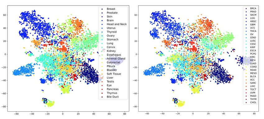
in most cases. Figure 2 shows the 2-D representation of obtained WSI embedding using
CNN-DS labelled based on primary site and primary diagnosis labels.
Lung cancer classification. The Lung Adenocarcinoma (LUAD) and Lung Squa-
mous Cell Carcinoma (LUSC) are two main cancer types of non-small cell lung cancer.
The classification of LUAD versus LUSC can aid pathologists in diagnosis of these cancer
subtypes that include 65-70% of all lung cancers (Zappa and Mousa, 2016). To validate
306CNN and Deep Sets for End-to-End Whole Slide Image Representation Learning
Table 1: Majority-3 and 5 search accuracy (%) for the horizontal search (primary site
identification) among 604 WSIs for Yottixel and CNN Deep Sets (best results in green).
Accuracy (in %)
Tumor Type Patient # Yottixel (k = 3) CNN-DS (k = 3) Yottixel (k = 5) CNN-DS (k = 5)
Brain 46 73 91 73 89
Breast 77 45 77 38 79
Endocrine 71 61 66 59 62
Gastro. 69 50 75 49 74
Gynaec. 18 16 33 0 27
Head/neck 23 17 69 13 65
Liver 44 43 56 36 43
Melanocytic 18 16 50 5 38
Mesenchymal 12 8 100 0 83
Prostate/testis 44 47 81 43 77
Pulmonary 68 58 91 54 89
Urinary tract 112 67 76 62 74
Table 2: Majority-3 and -5 search through k-NN for the vertical search among 604 WSIs.
Best F1-measure values highlighted.
F1-measure (in %)
Site Subtype nslides Yottixel CNN-DS Yottixel CNN-DS
LGG 23 78 89 75 81
Brain
GBM 23 82 89 83 84
THCA 50 92 98 91 98
Endocrine ACC 6 25 28 28 0
PCPG 15 61 81 61 79
ESCA 10 12 44 25 55
COAD 27 62 69 54 70
Gastro.
STAD 22 61 64 57 78
READ 10 30 55 16 0
UCS 3 75 80 50 50
Gynaeco. CESC 6 92 66 76 80
OV 9 80 82 66 82
CHOL 4 26 0 25 0
Liver, panc. LIHC 32 82 95 87 95
PAAD 8 94 94 77 94
PRAD 31 98 97 95 96
Prostate/testis
TGCT 13 96 93 86 93
LUAD 30 62 61 62 61
Pulmonary LUSC 35 69 60 69 62
MESO 3 0 50 0 0
BLCA 31 89 95 86 94
KIRC 47 91 87 89 84
Urinary tract
KIRP 25 75 84 79 81
KICH 9 70 53 66 0
the performance of CNN-DS, we apply it to LUAD/LUAC classification task. We gathered
2,580 (H&E) stained WSIs of lung cancer from TCGA repository. Among this, we employ
1,806 for training set and the remaining 774 WSIs for test set (Kalra et al., 2020a). The
patch selection and the architecture design of CNN-DS is the same as the one that used
in transfer learning task. We avoid training convolutional layers to have a fair comparison
against other transfer-learning based methods. The results have been reported in 3 where
CNN-DS can achieve competitive performance against the state-of-art.
307Hemati Kalra Tizhoosh
Table 3: CNN-DS evaluation on lung cancer classification via transfer learning.
Algorithm Accuracy (in %)
Coudray et al. (Coudray et al., 2018) 85
Kalra & Adnan et al. (Kalra et al., 2020a) 84
Khosravi et al. (Khosravi et al., 2018) 83
Yu et al. (Yu et al., 2016) 75
CNN-DS (Ours) 86
Figure 2: 2-D representation of obtained WSI embedding using CNN-DS labelled based on
24 primary sites (left) ad 30 primary diagnoses (right).
Query time comparison against Yottixel. We inteded to obtain one global repre-
sentation for a WSI. We argued that this is particularly useful for WSI search as the set
representation is bypassed. Hence, we measured query time for the leave-one-out approach
used for 604 WSIs. Results showed that while for Yottixel it takes around 16 minutes to
calculate pairwise distances between 604 WSIs, in our case it takes around 20 seconds to
reproduce the results.
6. Conclusions
We employed Deep Sets along with a CNN for end-to-end WSI representation. This was in-
spired by bag of patches (set) representation per WSI. Two reshape layers connected CNN
with Deep Sets. We propose to train our CNN-DS in the multi-label scheme. We used
the law of total probability to capture the primary site predicted probability for obtaining
probability of primary diagnosis. We validated the proposed topology in a transfer learning
scheme for WSI search. We showed that the proposed architecture can obtain WSI embed-
dings leading to comparable retrieval performance compared with Yottixel while reducing
the retrieval time significantly. We also applied the proposed scheme to lung classifcation
task and achieved competitive results compared with the state-of-art.
308CNN and Deep Sets for End-to-End Whole Slide Image Representation Learning
References
Alexander Buslaev, Vladimir I. Iglovikov, Eugene Khvedchenya, Alex Parinov, Mikhail
Druzhinin, and Alexandr A. Kalinin. Albumentations: Fast and flexible image augmen-
tations. Information, 11(2), 2020. ISSN 2078-2489. doi: 10.3390/info11020125. URL
https://www.mdpi.com/2078-2489/11/2/125.
Gabriele Campanella, Vitor Werneck Krauss Silva, and Thomas J Fuchs. Terabyte-scale
deep multiple instance learning for classification and localization in pathology. arXiv
preprint arXiv:1805.06983, 2018.
Wafa Chenni, Habib Herbi, Morteza Babaie, and Hamid R Tizhoosh. Patch clustering
for representation of histopathology images. In European Congress on Digital Pathology,
pages 28–37. Springer, 2019.
Lee Ad Cooper, Elizabeth G Demicco, Joel H Saltz, Reid T Powell, Arvind Rao, and
Alexander J Lazar. Pancancer insights from the cancer genome atlas: the pathologist’s
perspective. The Journal of pathology, 244(5):512–524, 2018.
Nicolas Coudray, Paolo Santiago Ocampo, Theodore Sakellaropoulos, Navneet Narula,
Matija Snuderl, David Fenyö, Andre L Moreira, Narges Razavian, and Aristotelis Tsiri-
gos. Classification and mutation prediction from non–small cell lung cancer histopathol-
ogy images using deep learning. Nature medicine, 24(10):1559–1567, 2018.
Thomas G Dietterich, Richard H Lathrop, and Tomás Lozano-Pérez. Solving the multiple
instance problem with axis-parallel rectangles. Artificial intelligence, 89(1-2):31–71, 1997.
Kevin Faust, Quin Xie, Dominick Han, Kartikay Goyle, Zoya Volynskaya, Ugljesa Djuric,
and Phedias Diamandis. Visualizing histopathologic deep learning classification and
anomaly detection using nonlinear feature space dimensionality reduction. BMC bioin-
formatics, 19(1):173, 2018.
Sobhan Hemati, Mohammad Hadi Mehdizavareh, Shojaeddin Chenouri, and Hamid R
Tizhoosh. A non-alternating graph hashing algorithm for large scale image search. arXiv
preprint arXiv:2012.13138, 2020.
Le Hou, Dimitris Samaras, Tahsin M Kurc, Yi Gao, James E Davis, and Joel H Saltz.
Patch-based convolutional neural network for whole slide tissue image classification. In
Proceedings of the IEEE conference on computer vision and pattern recognition, pages
2424–2433, 2016.
Maximilian Ilse, Jakub Tomczak, and Max Welling. Attention-based deep multiple instance
learning. In International conference on machine learning, pages 2127–2136. PMLR, 2018.
Shivam Kalra, Mohammed Adnan, Graham Taylor, and Hamid R Tizhoosh. Learning
permutation invariant representations using memory networks. In European Conference
on Computer Vision, pages 677–693. Springer, 2020a.
309Hemati Kalra Tizhoosh
Shivam Kalra, HR Tizhoosh, Charles Choi, Sultaan Shah, Phedias Diamandis, Clinton JV
Campbell, and Liron Pantanowitz. Yottixel–an image search engine for large archives of
histopathology whole slide images. Medical Image Analysis, 65:101757, 2020b.
Pegah Khosravi, Ehsan Kazemi, Marcin Imielinski, Olivier Elemento, and Iman Hajira-
souliha. Deep convolutional neural networks enable discrimination of heterogeneous dig-
ital pathology images. EBioMedicine, 27:317–328, 2018.
Diederik P Kingma and Jimmy Ba. Adam: A method for stochastic optimization. arXiv
preprint arXiv:1412.6980, 2014.
Bin Kong, Xin Wang, Zhongyu Li, Qi Song, and Shaoting Zhang. Cancer metastasis detec-
tion via spatially structured deep network. In International Conference on Information
Processing in Medical Imaging, pages 236–248. Springer, 2017.
Muhammad Khalid Khan Niazi, Anil V Parwani, and Metin N Gurcan. Digital pathology
and artificial intelligence. The lancet oncology, 20(5):e253–e261, 2019.
Gwenolé Quellec, Guy Cazuguel, Béatrice Cochener, and Mathieu Lamard. Multiple-
instance learning for medical image and video analysis. IEEE reviews in biomedical
engineering, 10:213–234, 2017.
Abtin Riasatian, Morteza Babaie, Danial Maleki, Shivam Kalra, Mojtaba Valipour, Sobhan
Hemati, Manit Zaveri, Amir Safarpoor, Sobhan Shafiei, Mehdi Afshari, et al. Fine-tuning
and training of densenet for histopathology image representation using tcga diagnostic
slides. arXiv preprint arXiv:2101.07903, 2021.
Mingxing Tan and Quoc Le. Efficientnet: Rethinking model scaling for convolutional neural
networks. In Int. Conf. on Machine Learning, pages 6105–6114. PMLR, 2019.
David Tellez, Geert Litjens, Jeroen van der Laak, and Francesco Ciompi. Neural image
compression for gigapixel histopathology image analysis. IEEE transactions on pattern
analysis and machine intelligence, 2019.
Hamid Reza Tizhoosh and Liron Pantanowitz. Artificial intelligence and digital pathology:
challenges and opportunities. Journal of pathology informatics, 9, 2018.
John N Weinstein, Eric A Collisson, Gordon B Mills, Kenna R Mills Shaw, Brad A Ozen-
berger, Kyle Ellrott, Ilya Shmulevich, Chris Sander, and Joshua M Stuart. The cancer
genome atlas pan-cancer analysis project. Nature genetics, 45(10):1113–1120, 2013.
Kun-Hsing Yu, Ce Zhang, Gerald J Berry, Russ B Altman, Christopher Ré, Daniel L Rubin,
and Michael Snyder. Predicting non-small cell lung cancer prognosis by fully automated
microscopic pathology image features. Nature communications, 7(1):1–10, 2016.
Manzil Zaheer, Satwik Kottur, Siamak Ravanbakhsh, Barnabas Poczos, Ruslan Salakhut-
dinov, and Alexander Smola. Deep sets. arXiv preprint arXiv:1703.06114, 2017.
Cecilia Zappa and Shaker A Mousa. Non-small cell lung cancer: current treatment and
future advances. Translational lung cancer research, 5(3):288, 2016.
310CNN and Deep Sets for End-to-End Whole Slide Image Representation Learning
In the following, the full description of the abbreviations for cancer subtypes in Table 2
have been presented in Table 4.
Table 4: Full description for primary diagnosis abbreviations used in the paper.
Abbreviation Primary Diagnosis
ACC Adrenocortical Carcinoma
BLCA Bladder Urothelial Carcinoma
CESC Cervical Squamous Cell Carcinoma and Endocervical Adenoc.
CHOL Cholangiocarcinoma
COAD Colon Adenocarcinoma
ESCA Esophageal Carcinoma
GBM Glioblastoma Multiforme
KICH Kidney Chromophobe
KIRC Kidney Renal Clear Cell Carcinoma
KIRP Kidney Renal Papillary Cell Carcinoma
LGG Brain Lower Grade Glioma
LIHC Liver Hepatocellular Carcinoma
LUAD Lung Adenocarcinoma
LUSC Lung Squamous Cell Carcinoma
MESO Mesothelioma
OV Ovarian Serous Cystadenocarcinoma
PAAD Pancreatic Adenocarcinoma
PCPG Pheochromocytoma and Paraganglioma
PRAD Prostate Adenocarcinoma
READ Rectum Adenocarcinoma
STAD Stomach Adenocarcinoma
TGCT Testicular Germ Cell Tumors
THCA Thyroid Carcinoma
UCS Uterine Carcinosarcoma
311You can also read