Optic Disc Preprocessing for Reliable Glaucoma Detection in Small Datasets
←
→
Page content transcription
If your browser does not render page correctly, please read the page content below

mathematics

Article
Optic Disc Preprocessing for Reliable Glaucoma Detection in
Small Datasets
José E. Valdez-Rodríguez                  , Edgardo M. Felipe-Riverón *           and Hiram Calvo *

                                           Centro de Investigación en Computación, Instituto Politécnico Nacional, Mexico City 07738, Mexico;
                                           jvaldezr1000@alumno.ipn.mx
                                           * Correspondence: edgardo@cic.ipn.mx (E.M.F.-R.); hcalvo@cic.ipn.mx (H.C.)

                                           Abstract: Glaucoma detection is an important task, as this disease can affect the optic nerve, and
                                           this could lead to blindness. This can be prevented with early diagnosis, periodic controls, and
                                           treatment so that it can be stopped and prevent visual loss. Usually, the detection of glaucoma is
                                           carried out through various examinations such as tonometry, gonioscopy, pachymetry, etc. In this
                                           work, we carry out this detection by using images obtained through retinal cameras, in which we can
                                           observe the state of the optic nerve. This work addresses an accurate diagnostic methodology based
                                           on Convolutional Neural Networks (CNNs) to classify these optical images. Most works require a
                                           large number of images to train their CNN architectures, and most of them use the whole image to
                                           perform the classification. We will use a small dataset containing 366 examples to train the proposed
                                           CNN architecture and we will only focus on the analysis of the optic disc by extracting it from the full
                                           image, as this is the element that provides the most information about glaucoma. We experiment with

                                           different RGB channels and their combinations from the optic disc, and additionally, we extract depth
                                    information. We obtain accuracy values of 0.945, by using the GB and the full RGB combination, and
Citation: Valdez-Rodríguez, J.E.;          0.934 for the grayscale transformation. Depth information did not help, as it limited the best accuracy
Felipe-Riverón, E.M.; Calvo, H. Optic      value to 0.934.
Disc Preprocessing for Reliable
Glaucoma Detection in Small                Keywords: glaucoma; convolutional neural networks; medical-diagnosis method; optic disc
Datasets. Mathematics 2021, 9, 2237.
https://doi.org/10.3390/math9182237

Academic Editors: Cornelio Yáñez           1. Introduction
Márquez, Yenny Villuendas-Rey and
                                                  Glaucoma is an illness that causes blindness in people of any age, but commonly in
Miltiadis D. Lytras
                                           older adults. This hereditary disease damages the eye’s optic nerve, which usually happens
                                           when fluid builds up in the front part of the eye. That extra fluid increases the pressure in
Received: 2 August 2021
Accepted: 10 September 2021
                                           the eye (aqueous humor), damaging the optic nerve. Although it is permanent damage
Published: 12 September 2021
                                           and cannot be reversed, medicine and surgery may help to stop further damage. That is
                                           why an early diagnosis of glaucoma is very important. The most common way of detecting
Publisher’s Note: MDPI stays neutral
                                           it is carried out through different analyses that involve the use of tools that are in contact
with regard to jurisdictional claims in
                                           with the patient’s eye, such as tonometry, that consists in applying a small amount of
published maps and institutional affil-    pressure to the eye by using a tonometer or by a warm puff of air, to measure the inner eye
iations.                                   pressure; ophthalmoscopy, that is a procedure that consists in dilating the pupil through
                                           eye drops, and examining the shape and color of the optic nerve; or gonioscopy, which
                                           aims to determine whether the angle where the iris meets the cornea is open and wide or
                                           narrow and closed, that defines the type of glaucoma, which is made by a hand-held contact
Copyright: © 2021 by the authors.
                                           lens placed on the eye (https://www.glaucoma.org/glaucoma/diagnostic-tests.php, last
Licensee MDPI, Basel, Switzerland.
                                           accessed 2 September 2021).
This article is an open access article
                                                  To detect glaucoma, in this work, digital retinal fundus images are required, as the
distributed under the terms and            glaucoma is mainly detected in the optic disc, through which the optic nerve transport to
conditions of the Creative Commons         the brain the visual information. The image of the optic disc provides the necessary infor-
Attribution (CC BY) license (https://      mation to detect glaucoma, as shown in Figure 1. In this work, we propose a methodology
creativecommons.org/licenses/by/           consisting in preprocessing digital images and extracting their color planes, to compare the
4.0/).                                     internal information this kind of image can contain. We focus our analysis on the optic disc

Mathematics 2021, 9, 2237. https://doi.org/10.3390/math9182237                                           https://www.mdpi.com/journal/mathematics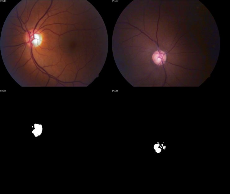
Mathematics 2021, 9, 2237                                                                                              2 of 14

                            by using some preprocessing techniques, as this element provides all the information about
                            the optic nerve and shows how glaucoma has evolved in the eye. Additionally, estimated
                            depth information will be added as an image to see if it can help the classification method-
                            ology, to correctly detect glaucoma by using Convolutional Neural Networks (CNNs).

                            Figure 1. Optic disc with normal cup and increased cup caused by glaucoma: (A,B) show optic discs
                            with normal cup and dimension quotes; (C,D) show optic discs with increased cup derived from
                            glaucoma. Image from [1].

                                 The content of this work is divided as follows: Section 2 shows some related works;
                            Section 3 describes the methodology employed in this work; Section 4 describes the
                            experiments carried out, and Section 5 presents the conclusions of the paper.

                            2. Related Work
                                 Glaucoma detection using CNNs is a common task in computer science, as many
                            solutions used so far have shown good results in classification tasks as mentioned by
                            Sultana et al. [2]; other recent works using CNNs to classify digital retinal fundus images
                            with glaucoma are mentioned below. Li et al. [3] use the Inception [4] CNN model trained
                            with their own private dataset; they trained it with the full RGB retinal fundus image and
                            classify them in positive or negative glaucoma. Fu et al. [5] created a four stage CNN
                            named DENet, that consists in first locating the optic disc in the full retinal fundus image,
                            then extract it and classify it; on the other hand, in another stage carries out a classification
                            from the full RGB retinal fundus images. Finally they obtain a final classification using the
                            results of the previous stages; to perform their experiments they used the SCES dataset [6].
                            Raghavendra et al. [7] proposes a CNN model composed of 18 layers trained with their
                            own dataset, using the full RGB image.
                                 Dos Santos Ferreira et al. [8] use a two stage methodology; the first one consists in
                            using the U-Net [9] model to extract a binary representation of the optic disc and the second
                            stage classifies this representation into two classes. They use the DRISHTI-GS dataset [10]
                            to perform their experiments. Christopher et al. [11] compare the results of different CNN
                            architectures such as VGG16 [12], Inception [4] and ResNet50 [13] with their own dataset.
                            Additionally, they mention the importance of data augmentation and transfer learning as
                            additional information for training the CNNs.
Mathematics 2021, 9, 2237                                                                                                 3 of 14

                                  Chai et al. [14] propose a multi-stage CNN trained with their own data, extracting
                            the first stage features from the full digital retinal fundus image; the second stage extracts
                            features from a subimage containing only the optic disc; the final stage joins both features
                            extracted from the previous stages and performs the classification using fully connected
                            layers. Bajwa et al. [15] propose a two-stage framework in which the first one consists
                            in extracting the area that contains the optic disc from the digital retinal fundus image
                            and the second stage consists in a CNN that extracts features and classifies them into two
                            classes. They use the DIARETDB1 dataset [16] to perform their experiments. Liu et al. [17]
                            use a large collection of own fundus images and the CNN model ResNet as classifier and
                            perform previously a statistical analysis on their data.
                                  Finally Barros et al. [1] perform a deep analysis on all the machine learning algorithms
                            and CNNs applied to glaucoma detection using many datasets. In Table 1 we show in an
                            arbitrary order a comparison amongst the results obtained from all previously mentioned
                            works, which were obtained according to the dataset each work used.

                            Table 1. Results obtained from the state of the art (higher is better [1]).

                              Paper                                Accuracy        Precision      Recall        Dataset
                              Liu et al. [17]                        0.9960          0.9770        0.9620       Private
                              Bajwa et al. [15]                      0.8740          0.8500        0.7117   DIARETDB1 [16]
                              Chai et al. [14]                       0.9151          0.9233        0.9090       Private
                              Chistopher et al. [11]                 0.9700          0.9300        0.9200       Private
                              Dos Santos Ferreira et al. [8]         1.0000          1.0000         1.000   DRISHTI-GS [10]
                              Raghavendra et al. [7]                 0.9813          0.9830        0.9800       Private
                              Fu et al. [5]                          0.9183          0.8380        0.8380      SCES [6]
                              Li et al. [3]                          0.9200          0.9560        0.9234       Private

                                 Although there are several works solving this task, the main problem is related to the
                            available data, because most of the datasets are private, due to lack of adequate public data;
                            another problem is that the CNN models used in many related works are complex models
                            that require high amounts of data (i.e., above 1000 images). In this work we propose the
                            use of a simple and accurate CNN model that can be trained with a low quantity of data
                            extracted from our own dataset.

                            3. Proposed Methodology
                                 The methodology used for this work consists of firstly preprocess the digital fundus
                            image with the purpose of obtaining useful information about glaucoma such that one
                            located in the optic disc. Once we have this information, we will use a CNN model
                            to estimate depth information from the extracted information. This depth information
                            consists in a representation of the distance between the user’s point of view and the objects
                            contained in the image; in this work we assume that the further object is the optic disc.
                            Finally, we set out to use all the visual information about the optic disc and depth estimation
                            in order to train a CNN capable to detect glaucoma.

                            3.1. Image Preprocessing
                                 Glaucoma is a disease that deteriorates the optic nerve that carries visual information
                            to the brain though the optic disc. For that reason we will focus our analysis precisely on
                            the optic disc. To perform its extraction automatically, digital image processing techniques
                            are used. Firstly we extract a Region of Interest (ROI) from the full retinal fundus image
                            containing the optic disc as it will be fed into a CNN to obtain the eventual presence of
                            glaucoma. In order to extract the ROI from the RGB image, we apply image thresholding
                            to the grayscale image in a simple and easy way, to obtain a binary representation of the
                            image; this binary representation contains clear information about the optic disc, as this is
                            always the brightest zone in the RGB image.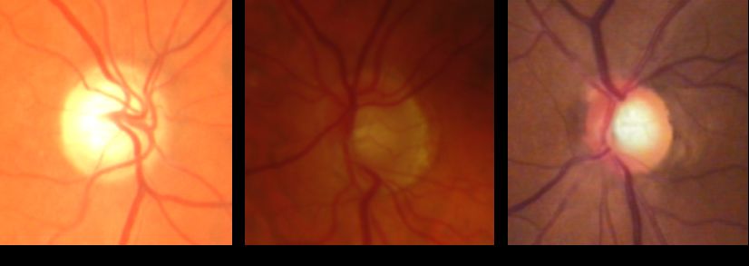
Mathematics 2021, 9, 2237                                                                                                4 of 14

                                  After obtaining this binary image showing clearly the optic disc, we compute the
                            centroid of it; then we align the center of the ROI with the previously calculated centroid
                            and extract a subimage from the original color image containing the optic disc, since it is the
                            only retinal element that contains information related to glaucoma in optical retinal images;
                            using only this patch as input of a CNN, we can classify the image if it is a glaucomatous
                            or non-glaucomatous one. In Figure 2 we show a resume of the preprocessing steps taken
                            in this work.
                                  In the next sections we will describe in detail the procedures that we have previously
                            exposed in general. As a first step before the preprocessing, we normalized the size of
                            all the images to 720 × 576 pixels, because the size may vary between all the images in
                            the dataset.

                            Figure 2. Preprocessing steps.

                            3.1.1. Image Thresholding
                                 Thresholding is the image processing operation that converts a multi-tone (graylevel)
                            image into a bi-tonal (binary) image. This was carried out by the well-known Otsu thresh-
                            old algorithm [18], TOtsu . It was derived from the histogram of the grayscale image intensity
                            values, h, which typically has L = 256 bins for 8-bit pixel images. Any chosen threshold
                            0 ≤ T ≤ L partitions the histogram into two segments: the optic disc and the back-
                            ground. The number of pixels w (Equation (1)), weighted mean intensity µ (Equation (2)),
                            and variance σ2 of both zones (Equation (3)), respectively, are given by:

                                                                         T −1                           L −1
                                                         w0 ( T ) =          ∑ h (i )      w1 ( T ) =   ∑ h (i )            (1)
                                                                             i =0                       i=T

                                                                         T −1                                 L −1
                                                                  1                                     1
                                                     µ0 ( T ) =
                                                                  w0     ∑ ih(i)           µ1 ( T ) =
                                                                                                        w1     ∑ ih(i)      (2)
                                                                         i =0                                  i=T
                                                                                    T −1
                                                                               1
                                                             σ02 ( T ) =
                                                                               w0   ∑ h(i)(i − µ0 (T ))2
                                                                                    i =0
                                                                                                                            (3)
                                                                                    L −1
                                                                           1
                                                             σ12 ( T )   =
                                                                           w1       ∑ h(i)(i − µ1 (T ))         2

                                                                                    i=T

                                The threshold of Otsu TOtsu (Equation (4)) was then defined as the threshold that
                            minimizes within-cluster variance:

                                                      TOtsu = argminw0 ( T )σ02 ( T ) + w1 ( T )σ12 ( T )                   (4)
                                                                         T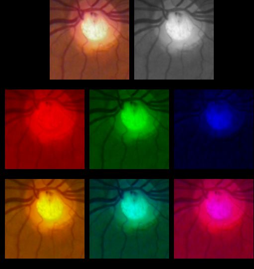
Mathematics 2021, 9, 2237                                                                                              5 of 14

                            or equivalently maximizes the between-cluster variance (Equation (5)), which reduces to:

                                                   TOtsu = argmaxw0 ( T )w1 ( T )(µ1 ( T ) − µ0 ( T ))2                   (5)
                                                                T

                                The search for TOtsu was performed by testing all values of T that minimized Equation (4)
                            or maximize Equation (5). Afterwards, thresholding (Equation (6)) was performed globally:

                                                                          0     I (i, j) < TOtsu
                                                          B(i, j) =                                                       (6)
                                                                          255   I (i, j) ≥ TOtsu

                            where (i, j) represent the pixel coordinates, I represents the actual grayscale value and B is
                            the resulting threshold value.
                                 Figure 3 presents as an example, the thresholding resulting from the graylevel image
                            obtained from the shown RGB image. Once the binary image was obtained, the centroid of
                            the binary image was calculated according to the procedure explained in Section 3.1.2.

                            Figure 3. Results of images thresholding, (A) RGB images, (B) Binary images.

                            3.1.2. Calculation of Centroids
                                 The centroid of a binary image is given by the arithmetic mean of the position of all
                            pixels that conformed to a shape of an object. Each shape contained in a binary image was
                            composed of white pixels, and the centroid is the average of the coordinates of all the white
                            pixels constituting the shape. On the other hand, an image moment is an average of all the
                            pixel intensities contained in an image. First we find the image moments µ0,0 , µ1,0 and µ0,1
                            of the binary image using Equations (7) and (8), where w is the width and h is the height of
                            the image. In this case, f takes the pixels on the ( x, y) coordinates with the value of 1 in the
                            object, as this operation is performed in a binary image:

                                                                            w    h
                                                                 µ0,0 =    ∑∑          f ( x, y)                          (7)
                                                                           x =0 y =0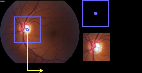
Mathematics 2021, 9, 2237                                                                                             6 of 14

                                                                       sum x            sumy
                                                              µ1,0 =           µ0,1 =                                    (8)
                                                                        µ0,0             µ0,0
                                 To obtain the sum of x and y coordinates of all white pixels, we used Equation (9):

                                                    sumx =   ∑ ∑ x f (x, y)    sumy =    ∑ ∑ y f (x, y)                  (9)

                                 Finally the coordinates of the centroid were given by Equation (10):
                                                                        µ10           µ01
                                                                 Cx =          Cy =                                    (10)
                                                                        µ00           µ00

                                 Cx is the x coordinate and Cy is the y coordinate of the centroid and µ denotes the
                            Moment (https://docs.opencv.org/3.4/dd/d49/tutorial_py_contour_features.html, last
                            accessed 2 September 2021).

                            3.1.3. Patch Extraction
                                 As we mentioned before, glaucoma manifests in the optic disc; sub-images are required
                            to be square for simplicity, given the circularity of optic discs. It is required to have an odd
                            number of pixels for the sub-image to have a center both horizontally and vertically. On the
                            other hand, the dimensions only depend on the size of the images and that of the optic disc
                            they contain. That is why we propose empirically a square ROI of 173 × 173 pixels. Once
                            we obtained Cx and Cy , we located them in the original image, we aligned the center of the
                            ROI Cx0 and Cy0 with Cx and Cy and extracted a subimage or patch of the full image that
                            contained the optic disc. Figure 4 depicts this operation.

                            Figure 4. Example of the alignment between the proposed ROI with the RGB image.

                            3.2. Depth Estimation
                                  Depth estimation was used to calculate the distance between the user’s point of view
                            and the object in the image; in the case of glaucoma classification, this cue was important
                            as it could show the status of the optic disc. As can be seen in Figure 5, depth information
                            can show a different perspective of the cup height inside the optic disc. The pixels with a
                            value near to 0 or black pixels represent the optic cup.
                                  In this work we used this cue as an additional input channel in order to add more
                            features to the RGB data. We obtained it using the proposal of Shankaranarayana et al. [19],
                            which consists of a CNN model capable of estimating depth from RGB images of the optic
                            disc. We implemented their model and trained it with the INSPIRE-stereo dataset [20] to
                            obtain the depth estimation. Once the network is trained, we obtained results from our
                            own dataset (see Section 4). Some examples are shown in Figure 6.
Mathematics 2021, 9, 2237                                                                                                7 of 14

                            Figure 5. Example of depth estimation of two optic discs. (A). Optic disc with glaucoma, (B). Optic
                            disc without glaucoma.

                            Figure 6. Depth estimation from the optic disc.

                            3.3. CNN Model
                                  The CNN model used in this work was based on the original AlexNet [21], given
                            that this model has shown good results in classification tasks [22–24]. This CNN consisted
                            of six convolutional layers with Rectified Linear Unit (ReLU) [25] as activation function
                            combined with Max-pooling layers used as feature extractors. After the convolutional
                            layers, as classification layer, we used two fully connected layers with 1024 neurons each
                            one with ReLU as activation function. The output of the model was obtained from two
                            neurons that classified if the retina presented glaucoma or not. The implementation of this
                            CNN model is shown in Figure 7.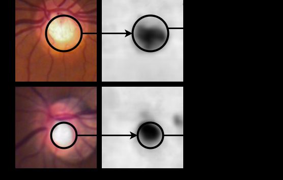
Mathematics 2021, 9, 2237                                                                                          8 of 14

                            Figure 7. AlexNet CNN model for glaucoma classification.

                            4. Experiments and Results
                                  In order to train the proposed CNN, we collected a private collection of retinal RGB
                            images from real patients, 257 images labeled as normal and 109 images with glaucoma
                            certified by two ophthalmologist specialists (Glaucoma Dataset, Centro de Investigación
                            en Computación, Instituto Politécnico Nacional, available at http://cscog.cic.ipn.mx/
                            glaucoma, last accessed 2 September 2021). This database (366 images) gathers images of
                            the retina of both eyes provided by two cooperating private ophthalmologists as specialists,
                            in a project on analysis of retinal images carried out a decade ago at the Computer Research
                            Center of the National Polytechnic Institute. These images were of specific patients of
                            both ophthalmologists, who, motivated by the due professional secrecy to which they
                            are due by their profession, were provided to us without details of the patients to whom
                            they belonged (name, sex, ages, systemic diseases they suffered, etc.). All the images
                            were of Mexican natives who came to them as patients, in order to be consulted to learn
                            about the disease that afflicted them when they noticed deficiencies in their vision systems,
                            namely, glaucoma, diabetic retinopathy, hypertensive retinopathy, retinitis pigmentosa,
                            among other. For us, knowing details of the images did not play any role in order to later
                            carry out statistical or other analyzes. The manual classification of the images was done by
                            the two ophthalmologists, which served for countless scientific publications as a result of
                            the automatic analysis of the system that was being developed at that time.
                                  We used data augmentation to randomly increase the amount of training data by
                            adding a modified version of the existing data; in our case we used the mirroring operation
                            done by reversing the pixels horizontally. In a horizontal mirroring, the pixel positions
                            located at coordinates ( x, y) were situated at coordinates (image_width − x − 1, y) in the
                            new image. In order to train the CNN model, we randomly divided the full dataset into a
                            training set (275 images) and testing set (91 images); we expanded the training set from
                            275 images to 550 images using the horizontal mirroring method.

                            4.1. Color Plane Extraction
                                 To help the CNN model classify color images for glaucoma detection, we decided to
                            extract and combine color planes obtained from the original RGB image and see if this
                            information may be useful for the task. In Figure 8 we show the images obtained from the
                            color planes and some of their combinations. Of them, we discarded the use of the red,
                            blue, and red + blue planes, due to the lack of information and low contrast for training.
                            This step was not contained in the preprocessing stage, because its main objective was the
                            extraction of the optic disc; we created a different dataset for each one of the extracted
                            planes from the optic disc image, i.e., we created a dataset for the red plane and the blue
                            plane separately. We also obtained the grayscale image by using the weighted method [26]:
Mathematics 2021, 9, 2237 9 of 14
Grayscale = 0.299R + 0.587G + 0.114B. In the CNN model, the input image had the follow
dimensions: 173 × 173 × c × n, where c = 1 when the input is the grayscale image or the
red, green or blue plane, c = 2 when the input was the combination of two color planes,
c = 3 when the input was the RGB image and c = 4 when the input was the RGB image
plus depth information.
Figure 8. Color planes extraction used for classification.
According to what we explained in previous section, we proposed the following
14 experiments: RGB and RGB-DA: training and testing with the original RGB image
with and without Data Augmentation (DA). RGB+Depth and RGB+Depth-DA: training
and testing with the original RGB image with depth estimation as additional information,
with and without DA. RGB+INV-Depth and RGB+INV-Depth-DA: training and testing
with the original RGB image with depth estimation as additional information but with
inverted gray levels, with and without DA. G and G-DA: training and testing with the
Green (G) plane of the image, with and without DA. GR and GR-DA: training and testing
with the (Green + Red) (GR) planes of the image, with and without DA. GB and GB-DA:
training and testing with the (Green + Blue) (GB) planes of the image, with and without
DA. Grayscale and Grayscale-DA: training and testing with the grayscale image, with and
without DA. In all the experiments the testing set contained 91 images; the training set
without DA contained 275 images, and 550 with DA.
4.2. Experimental Setup
The CNN training and implementation was carried out in a free GPU environment
using Google Colaboratory [27] with Tensorflow [23] and Keras (https://keras.io, last ac-
cessed 2 September 2021) frameworks. Firstly, we trained the depth estimation architec-Mathematics 2021, 9, 2237 10 of 14
ture; it took approximately 3 h for training and less than a second for testing a single
image. The training time for the experiments without data augmentation took approx-
imately 1 h and less than a second to test a single image. The training time for the
experiments with data augmentation took approximately 3 h and less than a second to
test a single image. The experiments that include depth information took similar time
for training and testing, with and without data augmentation respectively (code avail-
able at https://github.com/EduardoValdezRdz/Glaucoma-classification, last accessed 2
September 2021.)
4.3. Discussion
To evaluate our methodology we used state of the art metrics depicted in the follow-
ing equations:
True Positive + True Negative
Accuracy = (11)
True Positive + False Positive + False Negative + True Negative
True Positive
Precision = (12)
True Positive + False Positive
True Positive
Recall = (13)
True Positive + False Negative
Precision · Recall
F1 = 2 · (14)
Precision + Recall
Table 2 shows results for all performed experiments. We can see that, in general, data
augmentation was helpful and led into a better classification. RGB+Depth, RGB+INV-
Depth, G, GR led into a similar classification and we can say that these experiments could
be discarded and that depth information was not useful to classify glaucoma. We obtained
the best results using the original RGB image and the combination of the Green and
Blue planes, both with the augmented dataset. Using the grayscale image led to a good
classification of healthy cases.
Table 2. Quantitative results (higher is better).
Experiment Precision Recall Accuracy F1
RGB 0.7000 0.7777 0.8352 0.7368
RGB-DA 0.9230 0.8888 0.9450 0.9056
RGB+Depth 0.7500 0.7058 0.8351 0.6666
RGB+Depth-DA 0.9565 0.8148 0.9340 0.8800
RGB+INV-Depth 0.7500 0.7058 0.8351 0.6666
RGB+INV-Depth-DA 0.9565 0.8148 0.9340 0.8800
G 0.7727 0.6296 0.8352 0.6939
G-DA 0.8800 0.8148 0.9120 0.8561
GR 0.6111 0.8148 0.7912 0.6984
GR-DA 0.9565 0.8148 0.9340 0.8800
GB 0.9375 0.5555 0.8571 0.6977
GB-DA 0.9583 0.8518 0.9450 0.9019
Grayscale 0.7895 0.5555 0.8241 0.6522
Grayscale-DA 1 0.7777 0.9340 0.8750
Table 3 shows a relative comparison of results with similar works in the state of the
art, ordered by precision; however, it is important to note that this could not be a direct
comparison, as most datasets were private, and, although glaucoma-detection oriented,
they were not available to conduct tests directly. In terms of content, the state-of-the-art
datasets were similar since they all had fundus retinal images, the change between each
one of them was the number of images and their resolution. In general, the architecturesMathematics 2021, 9, 2237 11 of 14
of the previous works were complex models that required several training stages since
in intermediate stages they extract the optic disc and together with the complete image
perform their classification, except for Bajwa’s work in which is similar to ours, first he
uses a preprocessing to extract an image containing the optic disc and then his architecture
classifies images in which only the optic disc is presented, however our architecture showed
better results when classifying these images.
Table 3. Comparison between our best results vs. the state of the art (sorted by precision).
Paper Year Accuracy Precision Recall Model Images
Dos Santos
2018 1.0000 1.0000 1.0000 U-Net 101
Ferreira et al. [8]
Grayscale-DA
2021 0.9340 1.0000 0.7777 AlexNet 724
(ours)
Raghavendra
2018 0.9813 0.9830 0.9800 18-layer CNN 1426
et al. [7]
Liu et al. [17] 2019 0.9960 0.9770 0.9620 ResNet 274,413
GB-DA (ours) 2021 0.9450 0.9583 0.8518 AlexNet 724
Li et al. [3] 2018 0.9200 0.9560 0.9234 Inception-v3 70,000
Chistopher
2018 0.9700 0.9300 0.9200 ResNet50 4363
et al. [11]
Chai et al. [14] 2018 0.9151 0.9233 0.9090 MB-NN 2554
RGB-DA (ours) 2021 0.9450 0.9230 0.8888 AlexNet 724
Bajwa et al. [15] 2019 0.8740 0.8500 0.7117 7-layer CNN 780
Fu et al. [5] 2018 0.9183 0.8380 0.8380 DENet 1676
Finally, additional to these metrics, we were interested on examining the particular
number of false classifications our method found. True positives meant that a healthy optic
disc was classified as healthy; the true negatives mean that an optic disc with glaucoma
was classified as non-healthy; false positives meant that an optic disc with glaucoma was
classified as healthy; finally false negative meant that a healthy optic disc was classified
as non-healthy. In this work the worst case was the false positives, because a patient with
glaucoma could not be classified as healthy. In Figure 9 we show the values obtained in
our experiments. Another important point is that we identified some images that were not
classified correctly, because the images in question did not have the appropriate contrast to
be classified as depicted in Figure 10, since if they had high or low contrast the optic cup
was lost completely in the optic disc.Mathematics 2021, 9, 2237 12 of 14
Figure 9. Confusion matrices from some results; (b,l,n) are the best results.Mathematics 2021, 9, 2237 13 of 14
Figure 10. Comparison between high, low and adequate contrast images to be classified by the CNN.
5. Conclusions and Future Work
In this work, we presented a simple CNN model capable of classifying glaucoma in
digital retinal fundus color images, under low data conditions. This is achieved by first
extracting the optic disc from a full digital color image and other preprocessing methods
that we can apply to this type of image to perform a correct classification. Although the best
results in terms of accuracy were obtained using the original RGB image, the combination
of the Green and Blue planes also showed good results, due to the contrast of optic discs
that provide both images. Grayscale images allowed us to obtain a precision of 100%,
although with a corresponding decrease in recall. We found that adding depth information
was not helpful in the detection of glaucoma. The novelty of our work is based on the
comparison of different combinations of planes that can be obtained from an RGB image,
and although we show that the best results are obtained using the original image, the green
plane and its transformation to grayscale, we conclude that we can use a simple architecture
and still be able to adequately classify glaucoma. On the other hand, we identified the type
of images that can affect the performance of the classifiers. As future work, we propose
a further exploration of preprocessing methods to increase contrast and find the extent
to which the classification relies on. Although our method was successful with a small
number of images, as future work we plan to test the influence of extending the cases to be
tested in this task.
Author Contributions: Conceptualization, E.M.F.-R.; Formal analysis, E.M.F.-R.; Methodology, J.E.V.-R.;
Software, J.E.V.-R.; Supervision, H.C.; Validation, H.C.; Writing—original draft, J.E.V.-R.; Writing—
review and editing, E.M.F.-R. and H.C. All authors have read and agreed to the published version of
the manuscript.
Funding: This research was funded by the Government of Mexico via CONACYT, SNI, and Instituto
Politécnico Nacional (IPN) grants SIP 2083, SIP 20210189, SIP 20211425, IPN-COFAA and IPN-EDI,
and IPN-BEIFI.
Institutional Review Board Statement: Not applicable.
Informed Consent Statement: Informed consent was obtained from all subjects involved in the study.
Data Availability Statement: Dataset is available at: http://cscog.cic.ipn.mx/glaucoma; Code is
available at: https://github.com/EduardoValdezRdz/Glaucoma-classification.
Conflicts of Interest: The authors declare no conflict of interest.
References
1. Barros, D.M.; Moura, J.C.; Freire, C.R.; Taleb, A.C.; Valentim, R.A.; Morais, P.S. Machine learning applied to retinal image
processing for glaucoma detection: Review and perspective. BioMed. Eng. OnLine 2020, 19, 1–21. [CrossRef] [PubMed]
2. Sultana, F.; Sufian, A.; Dutta, P. Advancements in image classification using convolutional neural network. In Proceedings of the
2018 Fourth International Conference on Research in Computational Intelligence and Communication Networks (ICRCICN),
Kolkata, India, 22–23 November 2018, pp. 122–129.
3. Li, Z.; He, Y.; Keel, S.; Meng, W.; Chang, R.T.; He, M. Efficacy of a deep learning system for detecting glaucomatous optic
neuropathy based on color fundus photographs. Ophthalmology 2018, 125, 1199–1206. [CrossRef] [PubMed]Mathematics 2021, 9, 2237 14 of 14
4. Szegedy, C.; Liu, W.; Jia, Y.; Sermanet, P.; Reed, S.; Anguelov, D.; Erhan, D.; Vanhoucke, V.; Rabinovich, A. Going deeper with
convolutions. In Proceedings of the IEEE Conference on Computer Vision and Pattern Recognition, Boston, MA, USA, 7–15 June
2015; pp. 1–9.
5. Fu, H.; Cheng, J.; Xu, Y.; Zhang, C.; Wong, D.W.K.; Liu, J.; Cao, X. Disc-aware ensemble network for glaucoma screening from
fundus image. IEEE Trans. Med. Imaging 2018, 37, 2493–2501. [CrossRef] [PubMed]
6. Baskaran, M.; Foo, R.C.; Cheng, C.Y.; Narayanaswamy, A.K.; Zheng, Y.F.; Wu, R.; Saw, S.M.; Foster, P.J.; Wong, T.Y.; Aung, T. The
prevalence and types of glaucoma in an urban Chinese population: The Singapore Chinese eye study. JAMA Ophthalmol. 2015,
133, 874–880. [CrossRef] [PubMed]
7. Raghavendra, U.; Fujita, H.; Bhandary, S.V.; Gudigar, A.; Tan, J.H.; Acharya, U.R. Deep convolution neural network for accurate
diagnosis of glaucoma using digital fundus images. Inf. Sci. 2018, 441, 41–49. [CrossRef]
8. dos Santos Ferreira, M.V.; de Carvalho Filho, A.O.; de Sousa, A.D.; Silva, A.C.; Gattass, M. Convolutional neural network and
texture descriptor-based automatic detection and diagnosis of glaucoma. Expert Syst. Appl. 2018, 110, 250–263. [CrossRef]
9. Ronneberger, O.; Fischer, P.; Brox, T. U-net: Convolutional networks for biomedical image segmentation. In Proceedings of the
International Conference on Medical image Computing and Computer-Assisted Intervention, Lima, Peru, 4–8 October 2015;
pp. 234–241.
10. Sivaswamy, J.; Krishnadas, S.; Chakravarty, A.; Joshi, G.; Tabish, A.S. A comprehensive retinal image dataset for the assessment
of glaucoma from the optic nerve head analysis. JSM Biomed. Imaging Data Pap. 2015, 2, 1004.
11. Christopher, M.; Belghith, A.; Bowd, C.; Proudfoot, J.A.; Goldbaum, M.H.; Weinreb, R.N.; Girkin, C.A.; Liebmann, J.M.; Zangwill,
L.M. Performance of deep learning architectures and transfer learning for detecting glaucomatous optic neuropathy in fundus
photographs. Sci. Rep. 2018, 8, 1–13. [CrossRef] [PubMed]
12. Simonyan, K.; Zisserman, A. Very deep convolutional networks for large-scale image recognition. arXiv 2014, arXiv:1409.1556.
13. Szegedy, C.; Ioffe, S.; Vanhoucke, V.; Alemi, A. Inception-v4, inception-resnet and the impact of residual connections on learning.
In Proceedings of the AAAI Conference on Artificial Intelligence, San Francisco, CA, USA, 4–9 February 2017; Volume 31.
14. Chai, Y.; Liu, H.; Xu, J. Glaucoma diagnosis based on both hidden features and domain knowledge through deep learning models.
Knowl. Based Syst. 2018, 161, 147–156. [CrossRef]
15. Bajwa, M.N.; Malik, M.I.; Siddiqui, S.A.; Dengel, A.; Shafait, F.; Neumeier, W.; Ahmed, S. Two-stage framework for optic disc
localization and glaucoma classification in retinal fundus images using deep learning. BMC Med. Inform. Decis. Mak. 2019,
19, 136.
16. Kauppi, T.; Kalesnykiene, V.; Kamarainen, J.-K.; Lensu, L.; Sorri, I.; Raninen, A.; Voutilainen, R.; Uusitalo, H.; Kälviäinen, H.;
Pietilä, J. DIARETDB1 diabetic retinopathy database and evaluation protocol. In Medical Image Understanding and Analysis;
University of Wales: Aberystwyth, UK, 2007; Volume 2007, p. 61.
17. Liu, H.; Li, L.; Wormstone, I.M.; Qiao, C.; Zhang, C.; Liu, P.; Li, S.; Wang, H.; Mou, D.; Pang, R.; et al. Development and
validation of a deep learning system to detect glaucomatous optic neuropathy using fundus photographs. JAMA Ophthalmol.
2019, 137, 1353–1360. [CrossRef] [PubMed]
18. Otsu, N. A threshold selection method from gray-level histograms. IEEE Trans. Syst. Man Cybern. 1979, 9, 62–66. [CrossRef]
19. Shankaranarayana, S.M.; Ram, K.; Mitra, K.; Sivaprakasam, M. Fully convolutional networks for monocular retinal depth
estimation and optic disc-cup segmentation. IEEE J. Biomed. Health Inform. 2019, 23, 1417–1426. [CrossRef] [PubMed]
20. Tang, L.; Garvin, M.K.; Lee, K.; Alward, W.L.; Kwon, Y.H.; Abramoff, M.D. Robust multiscale stereo matching from fundus
images with radiometric differences. IEEE Trans. Pattern Anal. Mach. Intell. 2011, 33, 2245–2258. [CrossRef] [PubMed]
21. Krizhevsky, A.; Sutskever, I.; Hinton, G.E. ImageNet Classification with Deep Convolutional Neural Networks. In Advances in
Neural Information Processing Systems 25; Pereira, F., Burges, C.J.C., Bottou, L., Weinberger, K.Q., Eds.; Curran Associates, Inc.:
Red Hook, NY, USA, 2012; pp. 1097–1105.
22. Wang, S.; Kang, B.; Ma, J.; Zeng, X.; Xiao, M.; Guo, J.; Cai, M.; Yang, J.; Li, Y.; Meng, X.; et al. A deep learning algorithm using CT
images to screen for Corona Virus Disease (COVID-19). Eur. Radiol. 2021, 1–9. [CrossRef]
23. Abadi, M.; Barham, P.; Chen, J.; Chen, Z.; Davis, A.; Dean, J.; Devin, M.; Ghemawat, S.; Irving, G.; Isard, M.; et al. Tensorflow:
A system for large-scale machine learning. In Proceedings of the 12th USENIX symposium on operating systems design and
implementation (OSDI 16), Savannah, GA, USA, 2–4 November 2016; pp. 265–283.
24. Goodfellow, I.; Bengio, Y.; Courville, A.; Bengio, Y. Deep Learning; MIT Press: Cambridge, MA, USA, 2016; Volume 1,
25. Arora, R.; Basu, A.; Mianjy, P.; Mukherjee, A. Understanding Deep Neural Networks with Rectified Linear Units. arXiv 2016,
arXiv:1611.01491.
26. Gonzalez, R.C.; Woods, R.E. Digital Image Processing, 4th ed.; Prentice-Hall, Inc.: Upper Saddle River, NJ, USA, 2018.
27. Bisong, E. Google Colaboratory. In Building Machine Learning and Deep Learning Models on Google Cloud Platform: A Comprehensive
Guide for Beginners; Apress: Berkeley, CA, USA, 2019; pp. 59–64. [CrossRef]You can also read