Indoor Segmentation and Support Inference from RGBD Images
←
→
Page content transcription
If your browser does not render page correctly, please read the page content below
Indoor Segmentation and Support Inference
                   from RGBD Images

          Nathan Silberman1 , Derek Hoiem2 , Pushmeet Kohli3 , Rob Fergus1
                          1
                         Courant Institute, New York University
    2
        Department of Computer Science, University of Illinois at Urbana-Champaign
                           3
                             Microsoft Research, Cambridge

          Abstract. We present an approach to interpret the major surfaces, ob-
          jects, and support relations of an indoor scene from an RGBD image.
          Most existing work ignores physical interactions or is applied only to
          tidy rooms and hallways. Our goal is to parse typical, often messy, in-
          door scenes into floor, walls, supporting surfaces, and object regions, and
          to recover support relationships. One of our main interests is to better
          understand how 3D cues can best inform a structured 3D interpreta-
          tion. We also contribute a novel integer programming formulation to
          infer physical support relations. We offer a new dataset of 1449 RGBD
          images, capturing 464 diverse indoor scenes, with detailed annotations.
          Our experiments demonstrate our ability to infer support relations in
          complex scenes and verify that our 3D scene cues and inferred support
          lead to better object segmentation.

1       Introduction
Traditional approaches to scene understanding aim to provide labels for each
object in the image. However, this is an impoverished description since labels
tell us little about the physical relationships between objects, possible actions
that can be performed, or the geometric structure of the scene.
    Many robotics and scene understanding applications require a physical parse
of the scene into objects, surfaces, and their relations. A person walking into a
room, for example, might want to find his coffee cup and favorite book, grab
them, find a place to sit down, walk over, and sit down. These tasks require
parsing the scene into different objects and surfaces – the coffee cup must be
distinguished from surrounding objects and the supporting surface for example.
Some tasks also require understanding the interactions of scene elements: if the
coffee cup is supported by the book, then the cup must be lifted first.
    In this paper, our goal is to provide such a physical scene parse: to segment
visible regions into surfaces and objects and to infer their support relations. In
particular, we are interested in indoor scenes that reflect typical living conditions.
Challenges include the well-known difficulty of object segmentation, prevalence
of small objects, and heavy occlusion, which are all compounded by the mess
and disorder that are common in lived-in rooms. What makes interpretation
possible at all is the rich geometric structure: most rooms are composed of large
planar surfaces, such as the floor, walls, and table tops, and objects can often
be interpreted in relation to those surfaces. We can better interpret the room by
rectifying our visual data with the room’s geometric structure.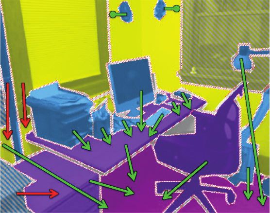
2       ECCV-12 submission ID 1079

    Our approach, illustrated in Fig. 1, is to first infer the overall 3D structure
of the scene and then jointly parse the image into separate objects and estimate
their support relations. Some tasks, such as estimating the floor orientation or
finding large planar surfaces are much easier with depth information, which is
easy to acquire indoors. But other tasks, such as segmenting and classifying
objects require appearance based cues. Thus, we use depth cues to sidestep
the common geometric challenges that bog down single-view image-based ap-
proaches, enabling a more detailed and accurate geometric structure. We are
then able to focus on properly leveraging this structure to jointly segment the
objects and infer support relations, using both image and depth cues. One of our
innovations is to classify objects into structural classes that reflect their physical
role in the scene: “ground”; “permanent structures” such as walls, ceilings, and
columns; large “furniture” such as tables, dressers, and counters; and “props”
which are easily movable objects. We show that these structural classes aid both
segmentation and support estimation.
    To reason about support, we introduce a principled approach that integrates
physical constraints (e.g. is the object close to its putative supporting object?)
and statistical priors on support relationships (e.g. mugs are often supported
by tables, but rarely by walls). Our method is designed for real-world scenes
that contain tens or hundred of objects with heavy occlusion and clutter. In
this setting, interfaces between objects are often not visible and thus must be
inferred. Even without occlusion, limited image resolution can make support
ambiguous, necessitating global reasoning between image regions. Real-world
images also contain significant variation in focal length. While wide-angle shots
contain many objects, narrow-angle views can also be challenging as important
structural elements of the scene, such as the floor, are not observed. Our scheme
is able to handle these situations by inferring the location of invisible elements
and how they interact with the visible components of the scene.

1.1   Related Work

Our overall approach of incorporating geometric priors to improve scene inter-
pretation is most related to a set of image-based single-view methods (e.g. [1–7]).
Our use of “structural classes”, such as “furniture” and “prop”, to improve seg-
mentation and support inference relates to the use of “geometric classes” [1]
to segment objects [8] or volumetric scene parses [3, 5–7]. Our goal of inferring
support relations is most closely related to Gupta et al. [6], who apply heuristics
inspired by physical reasoning to infer volumetric shapes, occlusion, and support
in outdoor scenes. Our 3D cues provide a much stronger basis for inference of
support, and our dataset enables us to train and evaluate support predictors
that can cope with scene clutter and invisible supporting regions. Russell and
Torralba [9] show how a dataset of user-annotated scenes can be used to infer
3D structure and support; our approach, in contrast, is fully automatic.
    Our approach to estimate geometric structure from depth cues is most closely
related to Zhang et al. [10]. After estimating depth from a camera on a mov-
ing vehicle, Zhang et al. use RANSAC to fit a ground plane and represent 3D
scene points relative to the ground and direction of the moving vehicle. We use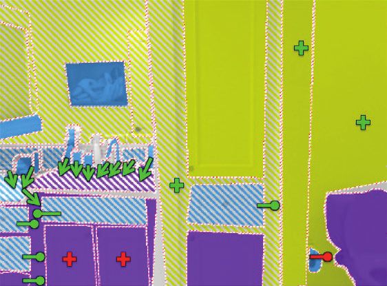
ECCV-12 submission ID 1079                                  3

        Input RGB                  Surface Normals                     Aligned Normals                  Segmentation

    Input Depth                    Inpainted Depth                        3D Planes                  Support Relations
                                Point Cloud                                                                               Structure
Image    1. Major Surfaces      RGB Image                    Regions                 Features                               Labels
         2. Surface Normals                   Segmentation               Feature                Support Classification
Depth    3. Align Point Cloud                                           Extraction                                        Support
Map
                                {Xi,Ni}                       {Rj}                    {Fj}                              Relationships

Fig. 1. Overview of algorithm. Our algorithm flows from left to right. Given an
input image with raw and inpainted depth maps, we compute surface normals and
align them to the room by finding three dominant orthogonal directions. We then
fit planes to the points using RANSAC and segment them based on depth and color
gradients. Given the 3D scene structure and initial estimates of physical support, we
then create a hierarchical segmentation and infer the support structure. In the surface
normal images, the absolute value of the three normal directions is stored in the R,
G, and B channels. The 3D planes are indicated by separate colors. Segmentation is
indicated by red boundaries. Arrows point from the supported object to the surface
that supports it.

RANSAC on 3D points to initialize plane fitting but also infer a segmentation
and improved plane parameters using a graph cut segmentation that accounts
for 3D position, 3D normal, and intensity gradients. Their application is pixel
labeling, but ours is parsing into regions and support relations. Others, such as
Silberman et al. [11] and Karayev et al. [12] use RGBD images from the Kinect
for object recognition, but do not consider tasks beyond category labeling.
    To summarize, the most original of our contributions is the inference of
support relations in complex indoor scenes. We incorporate geometric structure
inferred from depth, object properties encoded in our structural classes, and
data-driven scene priors, and our approach is robust to clutter, stacked objects,
and invisible supporting surfaces. We also contribute ideas for interpreting geo-
metric structure from a depth image, such as graph cut segmentation of planar
surfaces and ways to use the structure to improve segmentation. Finally, we offer
a new large dataset with registered RGBD images, detailed object labels, and
annotated physical relations.

2       Dataset for Indoor Scene Understanding
Several Kinect scene datasets have recently been introduced. However, the NYU
indoor scene dataset [11] has limited diversity (only 67 scenes); in the Berkeley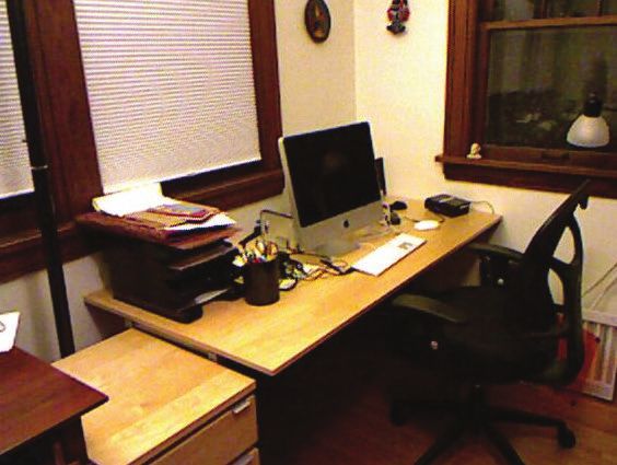
4        ECCV-12 submission ID 1079

Scenes dataset [12] only a few objects per scene are labeled; and others such
as [13, 14] are designed for robotics applications. We therefore introduce a new
Kinect dataset1 , significantly larger and more diverse than existing ones.
    The dataset consists of 1449 RGBD images2 , gathered from a wide range
of commercial and residential buildings in three different US cities, comprising
464 different indoor scenes across 26 scene classes.A dense per-pixel labeling was
obtained for each image using Amazon Mechanical Turk. If a scene contained
multiple instances of an object class, each instance received a unique instance
label, e.g. two different cups in the same image would be labeled: cup 1 and
cup 2, to uniquely identify them. The dataset contains 35,064 distinct objects,
spanning 894 different classes. For each of the 1449 images, support annotations
were manually added. Each image’s support annotations consists of a set of 3-
tuples: [Ri , Rj , type] where Ri is the region ID of the supported object, Rj is
the region ID of the supporting object and type indicates whether the support is
from below (e.g. cup on a table) or from behind (e.g. picture on a wall). Examples
of the dataset are found in Fig 7 (object category labels not shown).

3     Modeling the Structure of Indoor Scenes
Indoor scenes are usually arranged with respect to the orthogonal orientations
of the floor and walls and the major planar surfaces such as supporting surfaces,
floor, walls, and blocky furnishings. We treat initial inference of scene surfaces as
an alignment and segmentation problem. We first compute surface normals from
the depth image. Then, based on surface normals and straight lines, we find three
dominant and orthogonal scene directions and rotate the 3D coordinates to be
axis aligned with the principal directions. Finally, we propose 3D planes using
RANSAC on the 3D points and segment the visible regions into one of these
planes or background using graph cuts based on surface normals, 3D points, and
RGB gradients. Several examples are shown in Fig. 2. We now describe each
stage of this procedure in more detail.

3.1    Aligning to Room Coordinates
We are provided with registered RGB and depth images, with in-painted depth
pixels [15]. We compute 3D surface normals at each pixel by sampling surround-
ing pixels within a depth threshold and fitting a least squares plane. For each
pixel we have an image coordinate (u, v), 3D coordinate (X, Y , Z), and surface
normal (NX , NY , NZ ). Our first step is to align our 3D measurements to room
coordinates, so that the floor points upwards (NY =1) and each wall’s normal
is in the X or Z direction. Our alignment is based on the Manhattan world
assumption[16], that many visible surfaces will be along one of three orthogonal
directions. To obtain candidates for the principal directions, we extract straight
lines from the image and compute mean-shift modes of surface normals. Straight
line segments are extracted from the RGB image using the method described by
1
    http://cs.nyu.edu/~silberman/datasets/nyu_depth_v2.html
2
    640 × 480 resolution. The images were hand selected from 435, 103 video frames, to
    ensure diverse scene content and lack of similarity to other frames.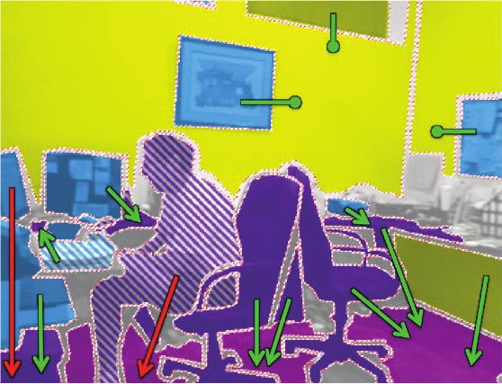
ECCV-12 submission ID 1079              5

 (a) Input RGB       (b) Normals        (c) Aligned     (d) RANSAC Fit (e) Segmented

Fig. 2. Scene Structure Estimation. Given an input image (a), we compute surface
normals (b) and align the normals (c) to the room. We then use RANSAC to generate
several plane candidates which are sorted by number of inliers (d). Finally, we segment
the visible portions of the planes using graph cuts (e). Top row: a typical indoor
scene with a rectangular layout. Bottom row: an scene with many oblique angles; floor
orientation is correctly recovered.
Kosecka et al. [17] and the 3D coordinates along each line are recorded. We com-
pute the 3D direction of each line using SVD to find the direction of maximum
variance. Typically, we have 100-200 candidates of principal directions. For each
candidate that is approximately in the Y direction, we sample two orthogonal
candidates and compute the score of the triple as follows:
                       3       NN                          NL
                      X     wN X       −(Ni · vj )2     wL X        (Li · vj )2
   S(v1 , v2 , v3 ) =     [       exp(              ) +       exp(−             )] (1)
                      j=1
                            NN i          σ2            NL i           σ2

    where v1 , v2 , v3 are the three principal directions, Ni is the surface normal
of a pixel, Li is the direction of a straight line, NN and NL are the number of
surface points and lines, and wN and wL are weights of the 3D normal and line
scores. In experiments, we set wN = 0.7, wL = 0.3, and σ = 0.01. We choose the
set of candidates that has the largest score, and denote them by vX , vY , and
vZ , where vY is chosen to be the direction closest to the original Y direction. We
can then align the 3D points, normals, and planes of the scene using the rotation
matrix R = [vX vY vZ ]. As shown in Fig. 3, the alignment procedure brings
80% of scene floors within < 5◦ of vertical, compared to 5% beforehand.
3.2 Proposing and Segmenting Planes                      1

We generate potential wall, floor, support, and        0.8
                                                         Percentage of Scenes

ceiling planes using a RANSAC procedure.
Several hundred points along the grid of pixel         0.6

coordinates are sampled, together with nearby          0.4
points at a fixed distance (e.g., 20 pixels) in
                                                       0.2                        Unaligned
the horizontal and vertical directions. While                                     Aligned
thousands of planes are proposed, only planes            0
                                                          0  5     10      15        20     25
above a threshold (2500) of inlier pixels after                Degrees from Vertical

RANSAC and non-maximal suppression are               Fig. 3. Alignment of Floors
retained.
    To determine which image pixels correspond to each plane, we solve a seg-
mentation using graph cuts with alpha expansion based on the 3D points X,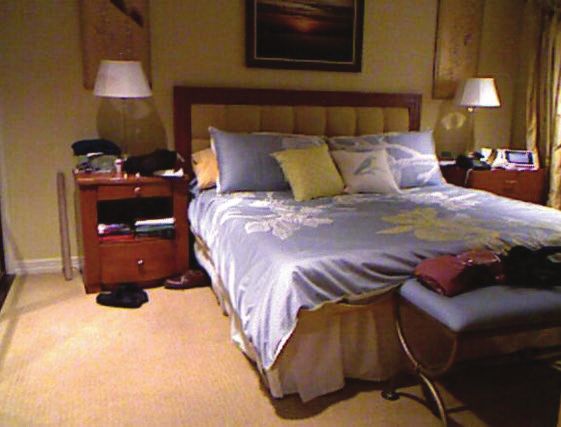
6       ECCV-12 submission ID 1079

Fig. 4. Segmentation Examples. We show two examples of hierarchical segmen-
tation. Starting with roughly 1500 superpixels (not shown), our algorithm iteratively
merges regions based on the likelihood of two regions belonging to the same object
instance. For the final segmentation, no two regions have greater than 50% chance of
being part of the same object.

the surface normals N and the RGB intensities I of each pixel. Each pixel i is
assigned a plane label yi = 0..Np for Np planes (yi = 0 signifies no plane) to
minimize the following
                   " energy:                              #
                     X                                       X
   E(data, y) = αi       f3d (Xi , yi ) + fnorm (Ni , yi ) +   fpair (yi , yj , I) (2)
                        i                                   i,j∈N8

     The unary terms f3d and fnorm encode whether the 3D values and normals
at a pixel match those of the plane. Each term is defined as log PPr(dist|outlier)
                                                                    r(dist|inlier)
                                                                                     ,
the log ratio of the probability of the distance between the pixel’s 3D position
or normal compared to that of the plane, given that the pixel is an inlier or
outlier. The probabilities are computed using histograms with 100 bins using the
RANSAC inlier/outlier estimates to initialize. The unary terms are weighted by
αi , according to whether we have directly recorded depth measurements (αi = 1),
inpainted depth measurements (αi = 0.25), or no depth measurements (αi = 0)
at each pixel. 1(.) is an indicator function. The pairwise term fpair (yi , yj , I) =
                    2
β1 + β2 ||Ii − Ij || enforces gradient-sensitive smoothing. In our experiments,
β1 = 1 and β2 = 45/µg , where µg is the average squared difference of intensity
values for pixels connected within N8 , the 8-connected neighborhood.
4    Segmentation
In order to classify objects and interpret their relations, we must first segment
the image into regions that correspond to individual object or surface instances.
Starting from an oversegmentation, pairs of regions are iteratively merged based
on learned similarities. The key element is a set of classifiers trained to predict
whether two regions correspond to the same object instance based on cues from
the RGB image, the depth image, and the estimated scene structure (Sec. 3).
   To create an initial set of regions, we use the watershed algorithm applied
to Pb boundaries, as first suggested by Arbeleaz [18]. We force this overseg-
mentation to be consistent with the 3D plane regions described in Sec. 3, which
primarily helps to avoid regions that span wall boundaries with faint intensity
edges. We also experimented with incorporating edges from depth or surface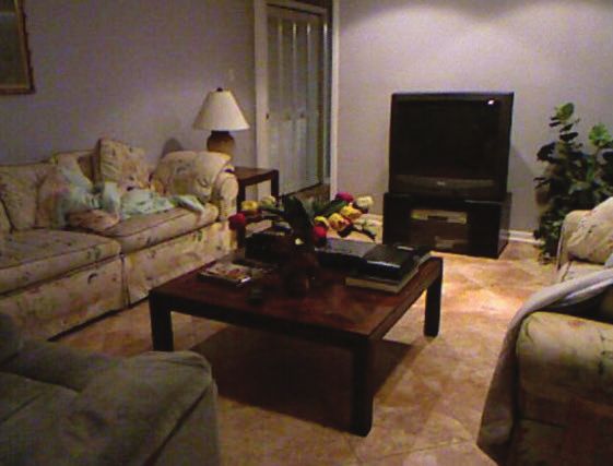
ECCV-12 submission ID 1079       7

orientation maps, but found them unhelpful, mostly because discontinuities in
depth or surface orientation are usually manifest as intensity discontinuities.
Our oversegmentation typically provides 1000-2000 regions, such that very few
regions overlap more than one object instance.
    For hierarchical segmentation, we adapt the algorithm and code of Hoiem et
al. [8]. Regions with minimum boundary strength are iteratively merged until
the minimum cost reaches a given threshold. Boundary strengths are predicted
by a trained boosted decision tree classifier as P(yi 6= yj |xsij ), where yi is the
instance label of the ith region and xsij are paired region features. The classifier
is trained using similar RGB and position features 3 to Hoiem et al. [8], but the
“geometric context” features are replaced with ones using more reliable depth-
based cues. These proposed 3D features encode regions corresponding to different
planes or having different surface orientations or depth differences are likely to
belong to different objects. Both types of features are important: 3D features
help differentiate between texture and objects edges, and standard 2D features
are crucial for nearby or touching objects.

5     Modeling Support Relationships
5.1 The Model
Given an image split into R regions, we denote by Si : i = 1..R the hidden
variable representing a region’s physical support relation. The basic assumption
made by our model is that every region is either (a) supported by a region visible
in the image plane, in which case Si ∈ {1..R}, (b) supported by an object not
visible in the image plane, Si = h, or (c) requires no support indicating that the
region is the ground itself, Si = g. Additionally, let Ti encode whether region i
is supported from below (Ti = 0) or supported from behind (Ti = 1).
    When inferring support, prior knowledge of object types can be reliable pre-
dictors of the likelihoods of support relations. For example, it is unlikely that
a piece of fruit is supporting a couch. However, rather that attempt to model
support in terms of object classes, we model each region’s structure class Mi ,
where Mi can take on one of the following values: Ground (Mi = 1), Furniture
(Mi = 2), Prop (Mi = 3) or Structure (Mi = 4). We map each object in our
densely labeled dataset to one of these four structure classes. Props are small
objects that can be easily carried; furniture are large objects that cannot. Struc-
ture refers to non-floor parts of a room (walls, ceiling, columns). We map each
object in our labeled dataset to one of these structure classes.
    We want to infer the most probable joint assignment of support regions S =
{S1 , ...SR }, support types T ∈ {0, 1}R and structure classes M ∈ {1..4}R . More
formally,

         {S∗ , T∗ , M∗ } = arg max P (S, T, M|I) = arg min E(S, T, M|I),        (3)
                              S,T,M                       S,T,M

where E(S, T, M|I) = − log P (S, T, M|I) is the energy of the labeling. The
posterior distribution of our model factorizes into likelihood and prior terms as
3
    A full list of features can be found in the supplementary material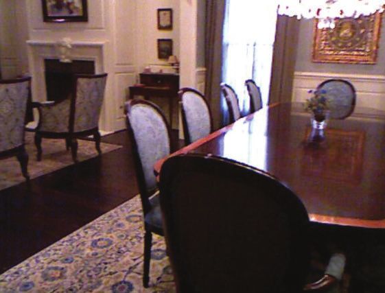
8        ECCV-12 submission ID 1079

                                    R
                                    Y
                P (S, T, M|I) ∝           P (I|Si , Ti )P (I|Mi ) P (S, T, M)          (4)
                                    i=1

to give the energy
                     R
                     X
                                    s
    E(S, T, M) = −         log(Ds (Fi,Si
                                         |Si , Ti )+log(Dm (Fim |Mi ))+EP (S, T, M). (5)
                     i=1

          S
where Fi,S  i
              are the support features for regions i and Si , and Ds is a Support
                                                 S
Relation classifier trained to maximize P (Fi,S    i
                                                     |Si , Ti ). FiM are the structure fea-
tures for region i and Dm is a Structure classifier trained to maximize P (FiM |Mi ).
The specifics regarding training and choice of features for both classifiers are
found in sections 5.3 and 5.4, respectively.
    The prior EP is composed of a number of different terms, and is formally
defined as:
                  XR
EP (S, T, M) =        ψT C (Mi , MSi , Ti ) + ψSC (Si , Ti ) + ψGC (Si , Mi ) + ψGGC (M).
                  i=1
                                                                               (6)
The transition prior, ψT C , encodes the probability of regions belonging to dif-
ferent structure classes supporting each other. It takes the following form:

                                       z∈supportLabels 1[z = [Mi , MSi , Ti ]]
                                      P
         ψT C (Mi , MSi , Ti ) ∝ − log P                                       (7)
                                         z∈supportLabels 1[z = [Mi , ∗, Ti ]]

The support consistency term, ψSC (Si , Ti ), ensures that the supported and
supporting regions are close to each other.  Formally, it is defined as:
                                     (Hib − HSt i )2 if Ti = 0,
                   ψSC (Si , Ti ) =                                       (8)
                                       V (i, Si )2   if Ti = 1,
where Hib and HSt i are the lowest and highest points in 3D of region i and Si re-
spectively, as measured from the ground, and V (i, Si ) is the minimum horizontal
distance between regions i and Si .
    The ground consistency term ψGC (Si , Mi ) has infinite cost if Si = g ∧ Mi 6=
1 and 0 cost otherwise, enforcing that all non-ground regions must be supported.
    The global ground consistency term ψGGC (M) ensures that the region
taking the floor label is lower than other regions in the scene. Formally, it is
defined as:                   R XR
                             X        κ if Mi = 1 ∧ Hib > Hjb
               ψGGC (M) =                                                      (9)
                                      0         otherwise,
                                 i=1 j=1

5.2 Integer Program Formulation
The maximum a posteriori (MAP) inference problem defined in equation (3) can
be formulated in terms of an integer program. This requires the introduction
of boolean indicator variables to represent the different configurations of the
unobserved variables S, M and T.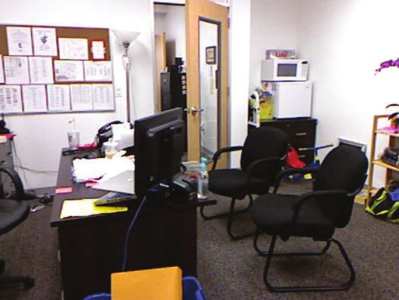
ECCV-12 submission ID 1079      9

    Let R0 = R + 1 be the total number of regions in the image plus a hidden
region assignment. For each region i, let boolean variables si,j : 1 ≤ j ≤ 2R0 + 1
represent both Si and Ti as follows: si,j : 1 < j ≤ R0 indicate that region i is
supported from below (Ti = 0) by regions {1, ..., R, h}. Next, si,j : R0 < j ≤ 2R0
indicate that region i is supported from behind (Ti = 1) by regions {1, ..., R, h}.
Finally, variable si,2R0 +1 indicates whether or not region i is the ground (Si = g).
    Further, we will use boolean variables mi,u = 1 to indicate that region i
                                                               u,v
belongs to structure class u, and indicator variables wi,j         to represent si,j = 1,
mi,u = 1 and mj,v = 1. Using this over-complete representation we can formulate
the MAP inference problem as an Integer Program using equations 10-16.
                                                              X             u,v
                        P        s
                                           P      m                w
             arg min       i,j θi,j si,j +  i,u θ i,u m i,u +     θi,j,u,v wi,j      (10)
                 s,m,w
                                                                i,j,u,v
                         P                 P
                  s.t.    j si,j = 1,           u mi,u = 1 ∀i                       (11)
                              P         u,v
                                 j,u,v wi,j     = 1,       ∀i                       (12)
                             si,2R0 +1 = mi,1 ,            ∀i                       (13)
                             P        u,v
                                u,v wi,j = si,j ,          ∀u, v                    (14)
                             P       u,v
                               j,v wi,j ≤ mi,u ,           ∀i, u                    (15)
                                          u,v
                         si,j , mi,u ,   wi,j   ∈ {0, 1}, ∀i, j, u, v               (16)

    The support likelihood Ds (eq. 5) and the support consistency ψSC (eq. 8)
                                                                             s
terms of the energy are encoded in the IP objective though coefficients θi,j   . The
structure class likelihood Dm (eq. 5) and the global ground consistency ψGGC
                                                                 m
(eq. 9) terms are encoded in the objective through coefficients θi,u . The transition
                                                      w
prior ψT C (eq. 7) is encoded using the parameters θi,j,u,v .
    Constraints 11 and 12 ensure that each region is assigned a single support,
type and structure label. Constraint 13 satisfies the Ground Consistency φGC
term (eq. ??). Constraints 14 and 15 are marginalization and consistency con-
straints. Finally, constraint 16 ensure that all indicator variables take integral
values. It is NP-hard to solve the integer program defined in equations 10-16. We
reformulate the constraints as a linear program, which we solve using Gurobi’s
LP solver, by relaxing the integrality constraints 16 to:
                                        u,v
                         si,j , mi,u , wi,j ∈ [0, 1],     ∀i, j, u, v.              (17)

    Fractional solutions are resolved by setting the most likely support, type and
structure class to 1 and the remaining values to zero. In our experiments, we
found this relation to be tight in that the duality gap was 0 in 1394/1449 images.
5.3 Support Features and Local Classification
Our support features capture individual and pairwise characteristics of regions.
                                                             s
Such characteristics are not symmetric: feature vector Fi,j     would be used to
determine whether i supports j but not vice versa. Geometrical features en-
code proximity and containment, e.g. whether one region contains another when
projected onto the ground plane. Shape features are important for capturing
characteristics of different supporting objects: objects that support others from
below have large horizontal components and those that support from behind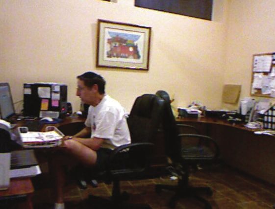
10        ECCV-12 submission ID 1079

have large vertical components. Finally, location features capture the absolute
3d locations of the candidate objects. 4
                                                                          S
    To train Ds , a logistic regression classifier, each feature vector Fi,j is paired
                     S
with a label Y ∈ {1..4} which indicates whether (1) i is supported from be-
low by j, (2) i is supported from behind by j, (3) j represents the ground
or (4) no relationship exists between the two regions. Predicting whether j
                                                                       S
is the ground is necessary for computing Ds (Si = g, Ti = 0; Fi,g        ) such that
                           S
P
   Si ,Ti D s (Si , Ti ; Fi,Si ) is a proper probability distribution.

5.4      Structure Class Features and Local Classification
Our structure class features are similar to those that have been used for object
classification in previous works [14]. They include SIFT features, histograms of
surface normals, 2D and 3D bounding box dimensions, color histograms [19] and
relative depth [11]4 . A logistic regression classifier is trained to predict the correct
structure class for each region of the image, and the output of the classifier is
interpreted as probability for the likelihood term Dm .
6      Experiments
6.1      Evaluating Segmentation
To evaluate our segmentation algorithm, we use the overlap criteria from [8]. As
shown in Table 1, the combination of RGB and Depth features outperform each
set of features individually by margins of 10% and 7%, respectively, using the
area-weighted score. We also performed two additional segmentation experiments
in which at each stage of the segmentation, we extracted and classified support
and structure class features from the intermediate segmentations and used the
support and structure classifier output as features for boundary classification.
The addition of these features both improve segmentation performance with
Support providing a slightly larger gain.
         Features                           Weighted Score Unweighted Score
         RGB Only                                52.5            48.7
         Depth Only                              55.9            47.3
         RGBD                                    62.7            52.7
         RGBD + Support                          63.4            53.7
         RGBD + Support + Structure classes      63.9            54.1
Table 1. Accuracy of hierarchical segmentation, measured as average overlap over
ground truth regions for best-matching segmented region, either weighted by pixel
area or unweighted.

6.2      Evaluating Support
Because the support labels are defined in terms of ground truth regions, we
must map the relationships onto the segmented regions. To avoid penalizing the
support inference for errors in the bottom up segmentation, the mapping is per-
formed as follows: each support label from the ground truth region [RiGT , RjGT , T ]
4
     A full list of features can be found in the supplementary material
ECCV-12 submission ID 1079 11
is replaced with a set of labels [RaS1 , RbS1 , T ]...[RaSw , RbSw , T ] where the overlap be-
tween supported regions (RiGT ,RaSw ) and supporting regions, (RjGT ,RbSw ) exceeds
a threshold (.25).
We evaluate our support inference model against several baselines:
– Image Plane Rules: A Floor Classifier is trained in order to assign Si = g
properly. For the remaining regions: if a region is completely surrounded by
another region in the image plane, then a support-from-behind relationship
is assigned to the pair with the smaller region as the supported region.
Otherwise, for each candidate region, choose the region directly below it as
its support from below.
– Structure Class Rules: A classifier is trained to predict each region’s
structure class. If a region is predicted to be a floor, Si = g is assigned.
Regions predicted to be of Structure class Furniture or Structure are assigned
the support of the nearest floor region. Finally, Props are assigned support
from below by the region directly beneath them in the image plane.
– Support Classifier: For each region in the image, we infer the likelihood
of support between it and every other region in the image using Ds and
assign each region the most likely support relation indicated by the support
classifier score.
The metric used for evaluation is the number of regions for which we predict
a correct support divided by the total number of regions which have a support
label. We also differentiate between Type Agnostic accuracy, in which we con-
sider a predicted support relation correct regardless of whether the support type
(below or from behind) matched the label and Type Aware accuracy in which
only a prediction of the correct type is considered a correct support prediction.
We also evaluate each method on both the ground truth regions and regions
generated by the bottom up segmentation.
Results for support classification are listed in Table 2. When using the ground
truth regions, the Image Plane Rules and Structure Class Rules perform well
given their simplicity. Indeed, when using ground truth regions, the Structure
Class Rules prove superior to the support classifier alone, demonstrating the use-
fulness of the Structure categories. However, both rule-based approaches cannot
handle occlusion well nor are they particularly good at inferring the type of
support involved. When considering the support type, our energy based model
improves on the Structure Class Rules by 9% and 17% when using the ground
truth and segmented regions, respectively, demonstrating the need to take into
account a combination of global reasoning and discriminative inference.
Visual examples are shown in Fig 7. They demonstrate that many objects,
such as the right dresser in the row3, column 3 and the chairs in row 5, column
1, are supported by regions that are far from them in the image plane, necessi-
tating non-local inference. One of the main stumbling blocks of the algorithm is
incorrect floor classification as show in the 3rd image of the last row. Incorrectly
labeling the rug as the floor creates a cascade of errors since the walls and bed
rely on this as support rather than using the true floor. Additionally, incorrect
structure class prediction can lead to incorrect support inference, such as the
objects on the table in row 4, column 1.12 ECCV-12 submission ID 1079
Predicting Support Relationships
Region Source Ground Truth Segmentation
Algorithm Type Agnostic Type Aware Type Agnostic Type Aware
Image Plane Rules 63.9 50.7 22.1 19.4
Structure Class Rules 72.0 57.7 45.8 41.4
Support Classifier 70.1 63.4 45.8 37.1
Energy Min (LP) 75.9 72.6 55.1 54.5
Table 2. Results of the various approaches to support inference. Accuracy is measured
by total regions whose support is correctly inferred divided by the number of labeled
regions. Type Aware accuracy penalized incorrect support type and Type Agnostic
does not.
I
magePl
aneRul
es St
ruct
ureCl
assRul
es Suppor
tCl
assi
f
ier Ener
gyMi
nimi
zat
i
on
Fig. 5. Comparison of support algorithms. Image Plane Rules incorrectly assigns many
support relationships. Structure Class Rules corrects several support relationships for
Furniture objects but struggles with Props. The Support classifier corrects several of the
Props but infers an implausible Furniture support. Finally, our LP solution correctly
assigns most of the support relationships. (→ : support from below, ( : support from
behind, + : support from hidden region. Correct support predictions in green, incorrect
in red. Ground in pink, Furniture in Purple, Props in Blue, Structure in Yellow, Grey
indicates missing structure class label. Incorrect structure predictions are striped.)
6.3 Evaluating Structure Class Prediction
To evaluate the structure class prediction, we calculate both the overall accuracy
and the mean diagonal of the confusion matrix. As 6 indicates, the LP solution
makes a small improvement over the local structure class prediction. Structure
class accuracy often struggles when the depth values are noisy or when the
segmentation incorrectly merges two regions of different structure class.
Ground .68 .28 .02 .02
Predicting Structure Classes
Labels
Overall Mean Class Furniture
.04 .70 .14 .12
Algorithm G. T. Seg. G. T. Seg. Prop
.03 .43 .42 .12
Classifier 79.9 58.7 79.2 59.0 Structure
.01 .24 .14 .59
Energy Min (LP) 80.3 58.6 80.3 59.6 Ground Furniture Prop Structure
Predictions
Fig. 6. Accuracy of the structure class recognition.
7 Conclusion
We have introduced a new dataset useful for various tasks including recogni-
tion, segmentation and inference of physical support relationships. Our dataset
is unique in the diversity and complexity of depicted indoor scenes, and we pro-
vide an approach to parse such complex environments through appearance cues,ECCV-12 submission ID 1079 13
room-aligned 3D cues, surface fitting, and scene priors. Our experiments show
that we can reliably infer the supporting region and the type of support, es-
pecially when segmentations are accurate. We also show that initial estimates
of support and major surfaces lead to better segmentation. Future work could
include inferring the full extent of objects and surfaces and categorizing objects.
Acknowledgements: This work was supported in part by NSF Awards 09-
04209, 09-16014 and IIS-1116923. The authors would also like to thank Microsoft
for their support. Part of this work was conducted while Rob Fergus and Derek
Hoiem were visiting researchers at Microsoft Research Cambridge.
References
1. Hoiem, D., Efros, A.A., Hebert, M.: Geometric context from a single image. In:
ICCV. (2005)
2. Hedau, V., Hoiem, D., Forsyth, D.: Recovering the spatial layout of cluttered
rooms. In: ICCV. (2009)
3. Hedau, V., Hoiem, D., Forsyth, D.: Thinking inside the box: Using appearance
models and context based on room geometry. In: ECCV. (2010)
4. Lee, D.C., Hebert, M., Kanade, T.: Geometric reasoning for single image structure
recovery. In: CVPR. (2009)
5. Lee, D.C., Gupta, A., Hebert, M., Kanade, T.: Estimating spatial layout of rooms
using volumetric reasoning about objects and surfaces. In: NIPS. (2010)
6. Gupta, A., Efros, A.A., Hebert, M.: Blocks world revisited: Image understanding
using qualitative geometry and mechanics. In: ECCV. (2010)
7. Gupta, A., Satkin, S., Efros, A.A., Hebert, M.: From 3d scene geometry to human
workspace. In: CVPR. (2011)
8. Hoiem, D., Efros, A.A., Hebert, M.: Recovering occlusion boundaries from an
image. Int. J. Comput. Vision 91 (2011) 328–346
9. Russell, B.C., Torralba, A.: Building a database of 3d scenes from user annotations.
In: CVPR. (2009)
10. Zhang, C., Wang, L., Yang, R.: Semantic segmentation of urban scenes using dense
depth maps. In: ECCV. (2010)
11. Silberman, N., Fergus, R.: Indoor scene segmentation using a structured light
sensor. In: ICCV Workshop on 3D Representation and Recognition. (2011)
12. Karayev, S., Janoch, A., Jia, Y., Barron, J., Fritz, M., Saenko, K., Darrell, T.: A
category-level 3-d database: Putting the kinect to work. In: ICCV Workshop on
Consumer Depth Cameras for Computer Vision. (2011)
13. Lai, K., Bo, L., Ren, X., Fox, D.: A large-scale hierarchical multi-view rgb-d object
dataset. In: ICRA. (2011)
14. Koppula, H., Anand, A., Joachims, T., Saxena, A.: Semantic labeling of 3d point
clouds for indoor scenes. In: NIPS. (2011)
15. Levin, A., Lischinski, D., Weiss, Y.: Colorization using optimization. In: SIG-
GRAPH. (2004)
16. Coughlan, J., Yuille, A.: Manhattan world: orientation and outlier detection by
Bayesian inference. Neural Computation 15 (2003)
17. Kosecka, J., Zhang, W.: Video compass. In: ECCV, Springer-Verlag (2002)
18. Arbelaez, P.: Boundary extraction in natural images using ultrametric contour
maps. In: Proc. POCV. (2006)
19. Tighe, J., Lazebnik, S.: Superparsing: scalable nonparametric image parsing with
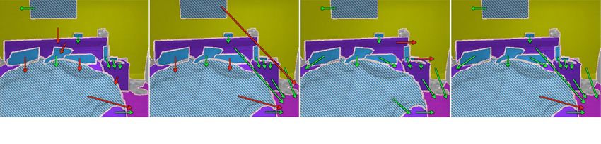
superpixels. In: ECCV, Berlin, Heidelberg, Springer-Verlag (2010) 352–36514 ECCV-12 submission ID 1079 Ground Truth Regions Segmented Regions Fig. 7. Examples of support and structure class inference with the LP solution. → : support from below, ( : support from behind, + : support from hidden region. Correct support predictions in green, incorrect in red. Ground in pink, Furniture in Purple, Props in Blue, Structure in Yellow, Grey indicates missing structure class label. Incorrect structure predictions are striped.
You can also read