Collateral Value Uncertainty and Mortgage Credit Provision
←
→
Page content transcription
If your browser does not render page correctly, please read the page content below
Collateral Value Uncertainty and Mortgage Credit Provision

                              Erica Xuewei Jiang and Anthony Lee Zhang∗

                                                January 2022

                                                    Abstract

       Using property transaction and financing data, we document large cross-sectional dif-
       ferences in how effective houses are as collateral for mortgages. Older and less stan-
       dardized houses tend to have higher price dispersion, and their appraisal values tend
       to deviate more from transaction prices. Mortgages collateralized by these houses are
       more likely to be rejected, have lower loan-to-price ratios, and higher risk-adjusted
       cost menu. This effect is stronger for home buyers with higher default risk, consistent
       with the collateral channel. We quantify the effect on homeownership gap using a life-
       cycle model with collateral constraints. We discuss the implications of our findings for
       FHA mortgage program, the shift from human to automated appraisals, and housing
       affordability policies.

   ∗
     Jiang is from the University of Southern California, Marshall School of Business. erica.jiang@marshall.usc.edu.
Zhang is from the University of Chicago Booth School of Business. anthony.zhang@chicagobooth.edu. Pranav Garg,
Willy Yu-Shiou Lin, and Michael Yip provided outstanding research assistance. We are grateful to Kenneth Ahern,
Jason Allen, Eric Budish, Sylvain Catherine, Scarlet Chen, Anthony DeFusco, Jason Donaldson, Marco Giacoletti,
Larry Harris, Mark Jansen, Gregor Matvos, Norm Miller, Andrii Parkhomenko, Giorgia Piacentino, Amir Sufi, Selale
Tuzel, Joe Vavra, Daniel Greenwald, Jinyuan Zhang, Arthur Korteweg, Rodney Ramcharan, participants at Columbia
Workshop in New Empirical Finance, the Guthrie Center Housing and Macroeconomics Conference, USC brownbag,
UIUC, and the Bank of Canada for comments. We are grateful for financial support from the Fama-Miller Center
for Research in Finance at the University of Chicago Booth School of Business. TransUnion (who provided some of
the data for this project) has the right to review the research before dissemination to ensure it accurately describes
TransUnion data, does not disclose confidential information, and does not contain material it deems to be misleading
or false regarding TransUnion, TransUnion’s partners, affiliates or customer base, or the consumer lending industry.
First version: August, 2021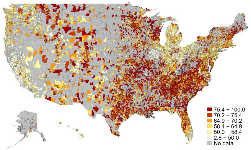
1      Introduction

The residential mortgage market has been central to policies for improving homeownership
and stabilizing the economy. Despite the significant amount of subsidies devoted to this
market, various frictions inhibit the passthrough of these subsidies to households (Glaeser
and Shapiro, 2003; Hurst et al., 2016; Agarwal et al., 2017; DeFusco, 2018; DeFusco and
Mondragon, 2020). Factors that prevent home buyers from borrowing against the house
can significantly affect their homeownership decisions, especially for low-income families.
Understanding such credit market frictions is important for improving homeownership rate,
a topic which has been central in housing policy debates.1
    In this paper, we document large cross-sectional differences in how effective houses are as
collateral for mortgages. Older and less standardized houses have higher price dispersion. We
show that the price dispersion of collateral affects financing: mortgages backed by houses
with high price dispersion have lower loan to price ratios, higher interest rates, and are
more likely to be rejected. This is true both in the private mortgage market, because value
uncertainty makes assets less effective as collateral, as well as in the government-backed
segment, due to the way that price dispersion interacts with the housing appraisal process.
Through a quantitative life-cycle model, we show that the borrowing constraints induced by
house price dispersion has a nontrivial effect on homeownership rates.
    Policymakers aiming to encourage homeownership for low-income households have con-
sidered interventions in credit markets as well as in housing markets. This paper highlights a
link between these two markets: the amount of credit that mortgage lenders provide depends
on the value uncertainty of the house used as collateral. We show that low-income house-
holds tend to live in areas with older and less standardized houses, which are intrinsically
difficult to lend against. Our findings provide a rationale for interventions in the mortgage
market, such as the FHA program, which allows low-income households to borrow at higher
LTV ratios. These policies alleviates a structural feature of the housing stock which limits
low-income households’ credit access even in efficient mortgage markets.
    The paper unfolds in two steps. First, we establish that collateral value uncertainty
affects home buyers’ mortgage credit access. We begin by using rich residential property
   1
     See policy reports, e.g., Herbert et al. (2005) and Boehm and Schlottmann (2008). As of 2021, homeownership rate
of below-median income households is about 52 percent, compared to 79 percent of above-median income households.
Source: The US Census quarterly report, Quarterly Residential Vacancies and Homeownership.

                                                         1
transaction data from 2000 to 2020 to document substantial cross-sectional variation in the
predictability of house prices. We find that older and less standardized houses in terms of
the number of bedrooms or square footage have more value uncertainty as measured by the
predicted pricing errors of a sophisticated hedonic model. Aggregating price dispersion to zip
code level, we show that zip code price dispersion is persistent over time. Thus, differences in
price dispersion across regions appear to be mainly driven by characteristics of local housing
stocks.
    We link property transaction data to mortgage records and show that collateral value
uncertainty affects financing at both the extensive margin and the intensive margin. At the
regional level, counties with higher price dispersion have more mortgage rejections, lower
average loan to price ratios conditional on loan approval, and higher interest rates. At
property level, comparing two houses which are transacted in the same zip-year at the same
transaction price, the house with higher estimated price dispersion tends to receive lower
loan-to-price ratios (LTPs). The result holds when we further restrict to comparing houses
financed by the same lender. One average, LTPs are 20-46bps lower for houses with one
standard deviation higher estimated price dispersion.
    Lower LTPs could in principle be caused by differences in credit demand rather than
credit supply: borrowers of houses with higher price dispersion could simply have lower
demand to borrow, causing them to substitute to smaller loans with lower interest rates. To
address this concern, using loan-level data, we estimate the menu of LTP-interest rate pairs
that are available in any given zip code-year. We find that, in high-dispersion zip codes, the
menu of risk-adjusted interest rate-LTP pairs shifts upwards: for any given LTP, borrowers
in high-dispersion zip codes can expect to pay higher risk-adjusted interest rates.
    We then show that the relationship between collateral value uncertainty and LTP is
stronger for borrowers with higher default risk, consistent with the collateral channel driving
our results. A one standard deviation increase in price dispersion induces a 42bp average
decrease in LTP for homebuyers with the highest credit scores, compared to a 110bp aver-
age effect for homebuyers with the lowest credit scores. The effect of credit scores on the
dispersion-relationship holds for both securitized and portfolio loans, but the effect is much
stronger for portfolio loans.
   We also show that mortgage applications in zip codes with higher house price dispersion
are more likely to be rejected. A one standard deviation increase in zip code average price

                                               2
dispersion is associated with a 1.4-1.8 percentage point increase in the mortgage rejection
rate, and an about 50bps increase in rejections explicitly attributable to problems with
collateral.
    The relationship between price dispersion and LTPs is plausibly driven by fair pricing of
debt for portfolio loans that banks keep on their balance sheets. However, it is unclear that
lenders have incentives to fairly price the effects of collateral dispersion in loans that they
plan to securitize (Hurst et al., 2016; Mian and Sufi, 2009; Keys et al., 2010; Purnanandam,
2011). We show that the dispersion-LTP relationship in the securitized segment of the market
works through the residential appraisal process. Securitizers set underwriting policies based
on the loan-to-value ratio of a house, which takes the loan amount divided by the minimum
value of the transaction price and the appraisal value. Appraisal values are based on recent
sale prices of comparable properties. When idiosyncratic price dispersion is higher, appraisal
values are noisier, creating downward pressure on the amount of loans that can be borrowed
against the underlying properties. Empirically, we show that house transactions receive
appraisals farther below their transaction prices in zip codes with higher price dispersion,
consistent with the appraisal channel.
    We perform three robustness tests of our results. First, we show that homebuyers of
houses with higher price dispersion are not more likely to default on their loans, suggesting
that our results are not driven by unobserved differences in borrowers’ creditworthiness that
are correlated with house price dispersion. Second, our results hold even with lender-zip-
year fixed effects, suggesting that the results are not driven by lender market power, or other
features of lenders’ behavior which affect all houses within a zipcode uniformly. Third, our
findings hold even restricting to a subsample of houses with sale prices below conforming
loan limits, suggesting that our findings are not driven by home buyers reducing borrowing
amounts to be eligible for GSE or FHA loans.
    In the second part of the paper, we build a life-cycle model of housing choice to show
how the variation in borrowing constraints induced by collateral value uncertainty influences
housing affordability and homeownership rates. In the model, households allocate stochastic
labor income between consumption and different qualities of housing over their lifecycles.
Households can borrow up to an LTV threshold, which is tied to the quality of the owned
housing. We evaluate the effects of collateral value variation by calibrating three versions
of the model, to areas with high, moderate, and low house price dispersion. We use our

                                              3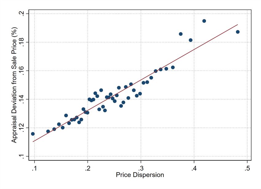
reduced-form estimates to inform the extent to which maximum mortgage LTVs vary across
these three scenarios. We find that moving from a high-dispersion county to a low-dispersion
county can increase aggregate homeownership rates by roughly 1.5pp, with larger effects on
poorer households (2.6pp), for whom down payment constraints are most binding.
    In support of our model results, we show empirically that counties with higher house
price dispersion have lower homeownership rates, controlling for household income and other
county characteristics. A 1SD increase in price dispersion is associated with approximately
a 1.3pp decrease in homeownership rates. Purging the difference in other county characteris-
tics, the effect of 1SD increase in dispersion on homeownership is 1pp greater for households
in the lowest income decile.
    Together, our results imply that the value uncertainty of the housing stock is a previously
overlooked variable which has quantitatively large effects on mortgage credit provision in
the US housing market. The value uncertainty channel is not a form of discrimination by
lenders, or an externality which can be addressed through Pigouvian taxation. Rather, it
is a structural phenomenon caused by intrinsic features of the housing stock: lenders in
competitive credit markets have higher costs of lending against poor collateral, and houses
tend to under-appraise by larger amounts, leading to lower credit provision for these houses.
    Our results have a number of policy implications. First, we provide a rationale for inter-
ventions, such as the FHA loan insurance program, which extend credit to low-income house-
holds and first-time homebuyers at loan-to-value ratios much higher than private lenders.
We have shown that low-income households face particularly high barriers to homeownership
because they tend to live in high-dispersion areas, so lack access to housing with high collat-
eral values. Thus, mortgage credit access is limited precisely for those households who are
most down-payment constrained, for whom credit is most valuable. Government interven-
tions to increase credit provision for low-income households, such as the FHA loan program,
can alleviate this effect.
    Second, our results suggest that the impending shift from human appraisals to automated
appraisals, such as the Desktop Appraisal program, may have adverse effects on mortgage
credit provision, especially for low-income households.2 Human appraisals are known to be
distorted upwards, so only a small share of houses under-appraise. Automated appraisals are
   2
     In 2021, the FHFA announced that banks and mortgage lenders could use automated appraisal software in place
of human appraisals.https://www.americanbanker.com/news/fhfa-will-make-desktop-home-appraisals-a-permanent-
option

                                                       4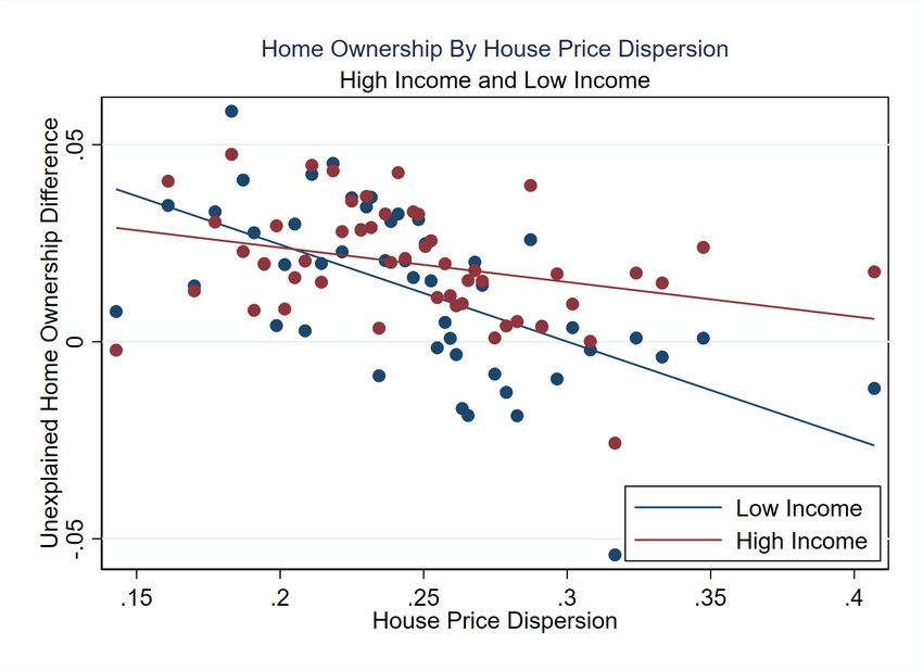
likely to be less distorted, but this may lead to a higher share of under-appraisals, especially
in areas where house price dispersion is high. Automating appraisals may thus actually
reduce credit access to low-income and minority households, who tend to live in areas with
high price dispersion.
    Finally, our results suggest that urban policymakers should consider the effects of their
policy instruments on how difficult it is to finance house purchases. In many parts of the
US, housing construction and renovation is highly regulated: local policymakers impose
restrictions on various characteristics of individual houses and also influence the overall rate
of renewal of the housing stock. These policies affect the overall value uncertainty of the
housing stock and thus how effective houses are as collateral for mortgage. Our results
imply that policies that encourage renewal of the housing stock, and promote construction
of cheap, homogeneous houses with predictable values could expand credit access, without
requiring the government to intervene directly in mortgage markets. These credit increases
are disproportionately valuable to low-income households, for whom credit is most important
for homeownership.
    This paper relates to a number of strands of literature. Broadly, our paper fits into
a literature on frictions that affect credit access. (Mian and Sufi, 2011; Agarwal et al.,
2017; Beraja et al., 2019; DeFusco et al., 2020; Buchak et al., 2018a; Jiang, 2020) and
homeownership (Glaeser and Shapiro, 2003). DeFusco and Mondragon (2020) study two
counter-cyclical refinancing frictions – the need to document employment and the need to
pay upfront closing costs – and show these frictions prevent borrowers who experience income
shocks to refinance. DeFusco (2018) studies how changes in access to housing collateral
affect homeowner borrowing behavior and estimate the marginal propensity to borrow out
of housing collateral. Greenwald (2016) uses a general equilibrium framework to study how
payment-to-income and loan-to-value ratios affect macroeconomic dynamics. We also relate
to a classic literature analyzing how collateral values affect the properties of debt contracts
collateralized by these assets or firms’ investment decisions (Titman and Wessels, 1988;
Shleifer and Vishny, 1992; Bian, 2021). Benmelech and Bergman (2008) analyzes the effect
of collateral liquidation values on contract renegotiation, and Benmelech and Bergman (2009)
studies how collateral values affect the cost of debt in the context of commercial real estate.
Our paper also builds on a literature on idiosyncratic price dispersion in the housing market
and its consequences. Case and Shiller (1989) and Giacoletti (2017) analyze idiosyncratic

                                               5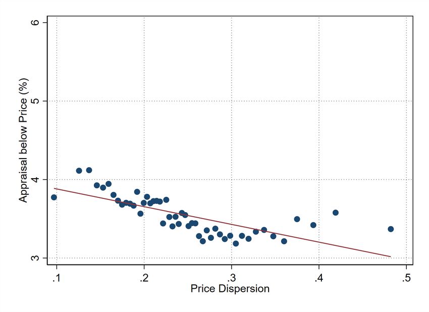
risk in residential real estate markets. Hartman-Glaser and Mann (2017) documents that
lower-income zip codes have more volatile returns to housing than higher-income zip codes.
They rationalize the finding with a model where shocks to the representative household’s
marginal rate of substitution lead to volatility in the return to housing via the collateral
constraint, and lower-incomes have a more volatile marginal rate of substitution, and thus
more volatile returns to housing. Sagi (2021) analyzes idiosyncratic risk in commercial real
estate. Sklarz and Miller (2016) propose a method to adjust loan-to-value ratios to reflect
house value uncertainty.
    The contribution of this paper is that we are the first to show that the collateral channel
matters in the US residential real estate market: there is substantial cross-sectional hetero-
geneity in housing collateral values, which affects mortgage credit availability and housing
affordability. Our analysis also elucidates the mechanisms through which the collateral chan-
nel influences outcomes within the unique structure of the US residential mortgage market:
in particular, how house price dispersion interacts with GSE securitization, regulatory con-
straints on banks, and the housing appraisal system to influence mortgage credit access.
    The paper proceeds as follows. Section 2 describes our data, measurement strategy, and
stylized facts on our price dispersion measure. Section 3 studies the effect of price dispersion
on mortgage provision. Section 4 calibrates a model to analyze the effect of collateral values
on homeownership rates. We discuss implications of our results in section 5, and conclude
in section 6.

2     Data and Measurement Strategy

2.1    Data Sources

   House Transaction Data. We use Corelogic Deed & Tax records data on housing
transactions in the US. We use data between 2000 and 2020 and restrict the sample to arms-
length, non-foreclosure transactions in single family residences. The date set reports each
house transaction attached to a specific property and provides information on sale amount,
mortgage amount, transaction date, and property location. We exclude transactions with
missing sale price, date, property ID, or location information. We merge the transaction
records with the Corelogic tax records to get property characteristics like year built and

                                               6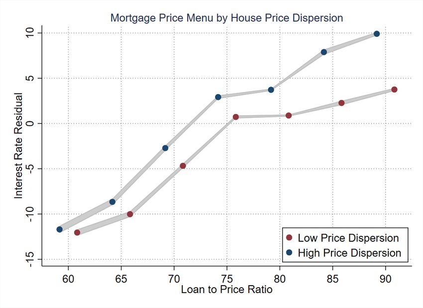
square footage. We provide detailed description about data cleaning steps in Appendix A.1.
    Mortgage Data. Besides the mortgage information in Corelogic Deeds, we use two
additional sources of mortgage data. First, we use the Corelogic Loan-Level Market Analytics
(LLMA) database. The database provides detailed information on mortgage and borrower
characteristics at origination – interest rates, down payments, sale prices, credit score, and
debt-to-income ratio – and monthly loan performance of the loan, including delinquency
status and investor type. Important for our analysis, the LLMA provides both appraised
house value and transaction price.
   Second, we use the Home Mortgage Disclosure Act (HMDA) for extensive margin analysis
on mortgage application rejections. The HMDA covers the near universe of U.S. mortgage
applications, including both originated and rejected applications. For rejected loans, we
observe the rejection reasons. Since we are not allowed to merge the LLMA and the Deeds
records, we aggregate the estimated idiosyncratic price dispersion, introduced in detail in
the next subsection, to the finest geographic regions in the LLMA (5-digit zip code) and in
the HMDA (census tract).
   Other Sources. We use the Booth TransUnion Consumer Credit Panel to calculate the
average VantageScore credit score by county to measure the creditworthiness of the entire
borrower population. We obtain zip level demographic data from the American Community
Survey (ACS) 1-year and 5-year samples.
   Table 1 provides summary statistics.

2.2    Measuring Value Uncertainty

We measure house value uncertainty as estimated idiosyncratic house price dispersion: which
types of houses have smaller pricing errors when priced with a hedonic regression. A similar
methodology is used in Buchak et al. (2020). Our methodology has two steps. First, we first
regress transaction prices on house characteristics:

                                  pit = ηkt + fk (xi , t) + it ,                          (1)

where i indexes properties, k indexes counties, and t indexes months. Equation 1 is effectively
a hedonic specification for house prices: log prices pit are determined by a county-month fixed

                                                7
effect, ηct , a smooth function fc (xi , t) of observable house characteristics xi and time t, and a
mean-zero error term it . ηct absorbs parallel shifts in log house prices in a county over time.
fc (xi , t) allows houses with different observable characteristics xi to appreciate at different
rates. For example, fc (xi , t) allows larger houses to appreciate faster than smaller houses,
or houses in the east of a certain county to appreciate faster than houses in the west.
   We then regress the squared residuals, ˆ2it , from (1), on a flexible function of characteristics
and time, to predict which house characteristics make them difficult to price:

                                                 ˆ2it = gc (xi , t) + ξit                                              (2)

where gc (xi , t), like fc (xi , t), is a generalized additive model in features, which we describe in
Appendix A.2. Using the estimates from this equation, we construct the predicted standard
deviation of the pricing error for every house:

                                                    σ̂it2 ≡ ĝc (xi , t)                                                (3)

The predicted values of idiosyncratic price dispersion at the house level, σ̂it2 , are our measure
of house value uncertainty. For ease of interpretation, we will generally take the square root
of σ̂it2 , which we call σ̂it , and use this in our analysis.
    Intuitively, specifications (1) and (2) is a heteroskedastic hedonic model of house prices:
they allow both the mean and idiosyncratic dispersion in house prices to be a function of
house characteristics. Specification (2) estimates, for a given house i, whether ˆ2it terms, the
squared errors from (1), tend to be large for houses with similar characteristics to i: that is,
whether i is priced with low error using a hedonic regression. As an example, suppose large
houses are more expensive than small houses, but also have lower price dispersion. fc (xi , t)
in specification (1) will be higher for large houses, capturing the fact that pit tends to be
higher for large houses. gc (xi , t) in specification (2) will tend to be smaller for large houses,
capturing the fact that the squared deviation of pit from its conditional mean (that is, the
hedonic model prediction) tends to be smaller for large houses.3
   3                                                                                            2
    Note that it is important to first run specification (2), using the predicted values of σ̂it  , rather than using the
                    2                                                                                            2
squared residuals ˆit in regressions directly. This is because the expected value of idiosyncratic dispersion, σit , is the
                                                                                       2                          2
analog of σ in our model, which is relevant for loan-to-values. Each realization of ˆit is a noisy measure of σit  . If we
regressed outcomes such as house-level LTP on the regression residuals ˆ2it directly, the coefficients would be biased
towards 0, relative to the first-best of regressing LTPs on σit , due to measurement error bias.

                                                             8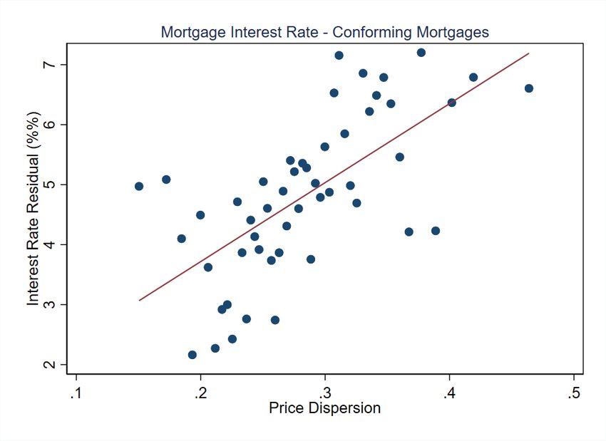
We use our estimates of price dispersion at the house level, and also at higher levels
of aggregation. For example, we will use σ̂c to denote the empirical estimate of standard
deviation of all ˆit terms in county c. σ̂c can be thought of as the log standard deviation of
house price residuals, after controlling for features in (1).

2.3    Estimated Value Uncertainty and Housing Market Frictions

We next present some stylized facts about the estimated value uncertainty of the US housing
stock over this time period, and discuss what housing market frictions are captured by the
estimated value uncertainty.
    Zip code level price dispersion is very persistent over time. Figure 1 plots zip-code
idiosyncratic price dispersion in 2020 (2010) against zip code dispersion in 2010 (2000).
Over both time periods, zip code dispersion in the later year is lined up with the dispersion
in the earlier year: regions with high price dispersion in 2000, for example, also have high
price dispersion in 2010. This suggests that the differences in price dispersion are driven
by persistent characteristics of a local housing stock rather than time-varying local market
condition.
    To explore this further, Table 2 presents the association between estimated value uncer-
tainty and house characteristics as well as local market conditions. Panel A analyzes house
features. Throughout, we control for linear and squared terms in log house prices, comparing
houses with similar prices and different characteristics. Column 1 shows that older houses
have higher price dispersion. We can partially measure house renovations, as the Corelogic
tax data contains an “effective year built” variable, which tracks the last date at which a
property was renovated. Columns 2 and 3 show that, controlling for the age of the building,
recently renovated houses – defined as houses with effective year built within 5 years of the
transaction date – have lower price dispersion, and houses which were ever renovated have
lower price dispersion.
   In columns 4-6, we analyze the association between building square footage and price
dispersion. There is a U-shaped relationship: price dispersion is low for moderately large
houses, and higher for houses which are very large or very small. Similarly, columns 5-6
show that 4-bedroom houses have lower price dispersion than houses with more or less than
4 bedrooms. In terms of local housing market conditions, Panel B of Table 2 shows that

                                              9
houses in zip codes with larger income inequality, less population density, and more vacancies
tend to have higher price dispersion.
Together, Table 2 suggests that house price dispersion is essentially driven by house
standardization and market thickness.4 Controlling for prices, houses which are newer,
located in densely populated areas, which are close to the median in terms of characteristics,
have lower price dispersion; older and less standardized houses have higher price dispersion.
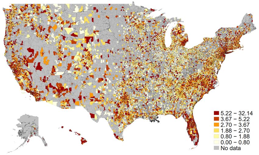
Figure 2 shows the relationship between price dispersion, average zipcode incomes, and
the zipcode minority share. Price dispersion tends to be higher in low-income, high-minority
share zipcodes. This is largely driven by the fact that price dispersion is generally decreasing
in prices, and house prices are very correlated with average incomes and minority shares
across zipcodes.
2.4 Drivers of Idiosyncratic Price Dispersion
Next, we discuss a number of factors and theoretical forces that may drive dispersion, and
explain why these theories have similar implications for mortgage credit provision.
Information asymmetry. Lenders of secured loans must be concerned about adverse
selection. This is especially the case in the consumer credit market, where houses and used
cars, for example, have diverse characteristics, some of which are difficult to measure, and
homeowners have better information about these characteristics (Kurlat and Stroebel, 2015;
Stroebel, 2016). Houses with more hard-to-measure characteristics tend to have higher value
uncertainty. Thus, lenders who lend against houses with higher value uncertainty may worry
more about adverse selection because the owners have more information advantage about
the house than the lenders.
Search frictions. The housing search literature has argued that house transaction
prices are not determined in a fully competitive and frictionless market. Prices appear to
depend not only on house characteristics: the transaction price of a house appears to be
causally influenced by characteristics of the buyer and seller. Sellers who are more patient
achieve higher sale prices, by setting higher list prices and keeping houses on the market
for longer; this has been shown using instruments for seller patience, such as homeowners’
4
This finding is consistent with evidence from other papers: see, for example, Kotova and Zhang (2021) and
Andersen et al. (2021).
10equity position (Genesove and Mayer, 1997; Guren, 2018) and homeowners’ nominal losses
since purchase (Genesove and Mayer, 2001). Using data from Norwegian housing auctions,
Anundsen et al. (2020) shows that the standard deviation of the ratio between buyers’
bid prices and appraisal values is approximately 7.9%, suggesting substantial dispersion in
buyers’ values for similar houses. Other factors, such as the experience of the realtor selling
the house, also appear to affect house sale probabilities and prices (Gilbukh and Goldsmith-
Pinkham, 2019).
Other factors. We also note that there are other possible housing market frictions which
generate price dispersion. The literature has studied many different models, such as random
search (Wheaton, 1990), directed search (Albrecht et al., 2016), and price posting (Guren,
2018). We do not take a stance on this paper on the particular theoretical microfoundation
of price dispersion, since it is not crucial for studying the effects of dispersion on credit
provision. As we argue in section 3.1 below, price dispersion decreases credit provision by
increasing lenders’ expected losses upon foreclosure, and by making appraisals noisier and
thus appraisal constraints more binding. Both effects occur regardless of the particular
theoretical microfoundation of prices dispersion.
If we observed all characteristics of houses that market participants observed, and our
functional forms for house prices were fully flexible, our measurement strategy would fully
filter out the effects of house characteristics, capturing only price dispersion generated by
housing market frictions. In practice, in addition to frictional price dispersion, our estimates
are likely to be confounded by two main factors. First, our estimation cannot account
for the effects of house characteristics unobserved in our data, but observed by market
participants. Second, our functional forms in (1) may not be flexible enough to capture
the true conditional expectation function; model misspecification will thus contribute to our
estimates of price dispersion. Both of these effects serve as confounds we would like to
filter out from our analysis, since if lenders use the correct price model with the full set
of observables, frictional price dispersion should affect mortgage lending decisions, but not
errors attributable to unobservables or model misspecification.
We believe these confounds are unlikely to drive our main results, for the following
reasons. We observe a rich set of characteristics, which are essentially all the features that
mortgage lenders observe for houses. A limitation of our data is that we only have time-
invariant do not observe renovations and time variation in house characteristics. However,
11Giacoletti (2017), using data on remodeling expenditures for houses in California appears
to have quantitatively small effects on estimated price: accounting for renovations decreases
the estimated standard deviation of returns by only around 2% of house prices.
3 House Value Uncertainty and Mortgage Credit
3.1 Theoretical Framework
We present a simple model illustrating how house value uncertainty affects mortgage credit
provision in Appendix B, and explain the main intuitions here. In our model, house value
uncertainty affects credit provision through two channels. The first channel, which we call
the fair pricing channel, is that each lender has some maximum amount she is willing to
lend against a given house for any given interest rate, which depends on how volatile the
foreclosure price of the house is. Formally, if the lender must foreclose and sell the house,
her payoff is concave in the house sale price: if the house sells for more than the outstanding
debt, the lender cannot keep the surplus, whereas if the house sells for less the lender is
on the hook for the difference. Thus, if the house price is more volatile, the lender expects
larger losses upon foreclosure, and thus must lower loan-to-value ratios to maintain a given
profit margin.5
The second channel, which we call the appraisal channel, is unique to the residential
housing market. Residential properties are appraised almost exclusively through comparable-
sales approach: appraisers identify similar properties which were transacted in recent months,
called “comps”, adjust the comparable properties’ prices for differences in characteristics
between the comp and the property to be appraised, and then take a weighted average of
comparables’ prices.6 Mortgage securitizers then set underwriting policies based on the loan-
to-value ratio of a house, where the value is calculated as the minimum of the transaction
price and the appraisal value. This minimum implies that values are a concave function of the
5
This argument is related to a large literature on collateral and debt (Williamson, 1988; Harris and Raviv, 1991;
Aghion and Bolton, 1992; Shleifer and Vishny, 1992; Hart and Moore, 1990; Bolton and Scharfstein, 1996; Diamond,
2004)
6
Appraisals are governed by the Uniform Standards of Professional Appraisal Practice (USPAP). The USPAP
identifies three allowable methods for assessment: a “sales comparison” approach, based on comparable sales; a
“cost” approach based on the cost of building the property, and an “income” approach based on the rental payment
flows from the property. In practice, residential real estate appraisal uses almost exclusively the sales comparison
approach.
12appraisal price: if the house over-appraises, the transaction price is used to determine loan-to-
values, whereas if the house under-appraises the appraisal binds. Thus, when idiosyncratic
price dispersion is high and appraisal values are noisier, there is downward pressure on
mortgage loan amounts.
Both the fair pricing and appraisal channels imply that houses with higher value uncer-
tainty are more difficult to lend against. Formally, the model makes three predictions. First,
for any given interest rate, loan-to-price ratios should be lower for houses with higher value
uncertainty. Second, mortgages are more likely to be rejected when value uncertainty is
higher. In the model, a mortgage application is rejected if the LTV that the buyer demands,
which depends on the buyer’s cash-on-hand for down payments, is higher than the maximum
LTV that the lender offers. When house value uncertainty is higher, lenders’ LTV limits will
be lower, so a larger fraction of mortgage applications will be rejected. Lastly, the rela-
tionship between value uncertainty and LTPs should be stronger for borrowers with higher
default risks. This is because, in the fair pricing channel, the value of collateral matters only
if consumers actually default: for prime consumers with low default rates, LTPs will tend to
be both higher and less sensitive to default rates. We proceed to show that these predictions
hold empirically.
3.2 County-Level Evidence
We begin with county-level evidence in Figure 3. We show that counties with higher price
dispersion have lower average loan-to-price ratios, higher interest rates, and more mortgage
rejections.
Panel (a) of Figure 3 plots county average loan to house price (LTP) against the average
house value uncertainty after controlling for local house prices. There is a robust negative
relationship: counties with higher house value uncertainty have lower average loan-to-price
ratios. In Figure A7, we show that the relationship holds for GSE loans, FHA loans, and
jumbo loans. Figure A8 confirms the negative relationship using residualized LTP, by taking
the residuals of regressions of LTP on mortgage interest rate, debt-to-income ratio (DTI),
DTI-square, FICO, FICO-square, log house price, and their interactions with origination
years, and origination year fixed effects.
Panel (b) of Figure 3 plots county average residualized mortgage rate against the average
13house price dispersion. We residualize rates for individual mortgages on borrower and loan
characteristics such as FICO, LTP, DTI, the squared terms, and their interactions with
origination year. We find that interest rates are higher in areas with higher price dispersion.
In other words, mortgages in high-dispersion areas are worse for borrowers along both the
price and LTP dimensions. This is inconsistent with the hypothesis that the relationship
between LTP and dispersion is driven by lower demand for credit in areas with lower price
dispersion, rather than lenders being less willing to supply credit. If lower LTPs reflect lower
credit demand, interest rates should also be lower in areas with higher price dispersion,
since home buyers on average are taking out safer, better-collateralized mortgages. Figure
A9 shows that the relationship holds for GSE loans, FHA loans, and jumbo loans. We
will show further evidence for this in Figure 5 below, which shows that the menu of LTP-
interest rate pairs offered in high-dispersion areas appears to be uniformly less favorable for
borrowers.
Panels (c) and (d) of Figure 3 plot county-level average mortgage rejection rates against
county-level price dispersion. Panel (c) shows all mortgage rejections, and panel (d) considers
only mortgage rejections which are tied to collateral quality. We calculate rejection rates by
taking the total number of rejected mortgages, and dividing by the total number of mortgages
in the HMDA data. We residualize mortgage rejection rates, by taking the residuals from
a regression on average log house prices, credit scores, and year fixed effects. Consistent
with the extensive margin prediction, mortgage rejection rates are higher in counties with
higher price dispersion. In particular, the fraction of mortgages rejected for collateral-related
reasons is higher in high-dispersion counties.
3.3 Property-Level Evidence
We next turn to property level evidence, which allows us to exploit within-county variation
and better control for borrower characteristics for identification.
3.3.1 Loan-to-Price Ratio
We start with the effect of collateral value uncertainty on property-level LTP. We first visu-
alize the relationship between property-level LTP and collateral value uncertainty in Figure
144. To compare properties within a county, we regress LTP, and predicted house price disper-
sion from specification (3), on house prices and county-year fixed effects, and plot the LTP
residuals against house price dispersion residuals. Figure 4 shows a clear negative association
between LTP and collateral value uncertainty: houses with higher predicted price dispersion
receive less credit than other houses in the same county and transacted in the same year.
Formally, we estimate the following property-level specification:
LT Pikt = α + βDispersionikt + Xikt Γ + µkt + νm + ikt (4)
LT Pikt and Dispersionikt are the loan-to-sale price ratio and the estimated price dispersion,
respectively, of property i in county k sold in year t. Xikt is a set of property and zip-code
level controls. Specifically, we include the transaction price of the property, mortgage type,
mortgage term, and resale indicator. µkt and νm are county-year and transaction month
fixed effects, respectively.
Table 3 reports the results. We first confirm the effect of house price dispersion on
mortgage loan-to-price ratio in a less saturated specification by including only loan controls
in column 1. For two houses with the same transaction price, the one with higher estimated
price dispersion tends to receive a smaller sized loan. The result holds in more saturated
specifications with transaction date fixed effects (column 2), plus county-year fixed effects
(column 3), plus lender-year fixed effects (column 4), and when we county-year with zip-year
fixed effects (column 5). The loan-to-price ratio is about 20-46bps lower for houses with one
standard deviation higher estimated price dispersion across these specifications.
3.3.2 Mortgage Price Menus
Once again, lower LTPs could be explained by credit demand: borrowers of houses with
higher price dispersion could simply have lower demand to borrow, and thus substitute to
smaller loans with lower interest rates. Using property-level data, we can evaluate this
hypothesis by estimating the entire menu of LTP-interest rate pairs that are available in a
market. Figure 5 plots the mortgage price menu, separately for groups of zip codes with high
and low price dispersion. Formally, we first residualize interest rates on borrowers’ credit
scores, a dummy for conforming vs jumbo loans, and then a time fixed effect; and then plot
a menu of average interest rates for different LTPs. Figure 5 shows that, in high-dispersion
15zip codes, the entire menu of interest rate-LTP pairs shifts upwards: for any given LTP,
borrowers in high-dispersion zip codes can expect to pay higher prices. The difference is
about 3bps for loans with LTP below 80 and enlarges to 8bps for loans with LTP above 80.
Next, we estimate the following loan-level specifications:
Rateikt = α + βLT Pikt + γZipDispersionikt + Xikt Γ + µkt + νm + ikt
(5)
LT Pikt = α + βRateikt + γZipDispersionikt + Xikt Γ + µkt + νm + ikt
Rateikt is property i’s mortgage rate. LT Pikt is the loan-to-sale price ratio of property i in
county k. ZipDispersionikt is the zip code average price dispersion. Xikt is a set of property
and zip-code level controls. Specifically, we include the transaction price of the property,
borrower credit score, credit score squared, debt-to-income ratio (DTI), DTI-squared, and
loan type. µkt and num are county-year and transaction month fixed effects, respectively.
Table 4 reports the cost menu results. Panel A shows the interest rate results. Column
1 uses the full sample. We first confirm that higher loan-to-price ratios are associated with
higher interest rates. The coefficient on LTP is positive and statistically significant. A one
percentage point increase in LTP is associated with about 0.85bps increase in interest rate.
Controlling for LTP, houses in zip codes with higher house price dispersion are financed
with more expensive mortgages. The mortgage rate increases by 1.1bps in zip codes with
one standard deviation higher average house price dispersion. Columns 2 to 4 shows the
results for GSE loans, FHA loans, and portfolio loans, respectively. The results hold in all
samples. For every one standard deviation higher zip-code average house price dispersion, the
mortgage rate of GSE loans increases by 1.24bps, the mortgage rate of FHA loans increases
by 1.23bps, and the mortgage rate of the portfolio loans increases by 0.43bps.
Panel B of Table 4 shows that to receive the same mortgage rate, houses with more higher
price dispersion require more down payment. Controlling for interest rate, the loan-to-price
ratios decrease by about 50bps in zip codes with one standard deviation higher average
house price dispersion (column 1). The results hold for GSE loans, FHA loans, and portfolio
loans (columns 2-4). For every one standard deviation higher zip-code average house price
dispersion, the LTP ratios of GSE loans decrease by 44bps, the LTP ratios of FHA loans
decrease by 22bps, and the LTP of portfolio loans decrease by 57bps.
163.3.3 Mortgage Rejection Rates
Next, we study the effect of price dispersion on credit access at the extensive margin. Lenders
require larger down payments when appraisal values are more likely to deviate from the sale
price. If borrowers are facing budget constraints and thus cannot make bigger down payment,
their mortgage applications may be rejected. We test this prediction by estimating the
following specification:
Rejectionijkt = α + βZipDispersionikt + Xikt Γ + µkt + νjt + ikt (6)
Rejectionikt is an indicator for whether a mortgage application from borrower i in county
k in year t is rejected. ZipDispersionikt is the zip code average price dispersion. Xikt is
a set of property and zip-code level controls. Specifically, we include zip code house price,
log of borrower income, loan type, county average credit score and its square term, and
loan-to-income ratio and its square term. µkt and νjt are county-year and lender-year fixed
effects, respectively.
Panel A of Table 5 reports the results. We first confirm the effect of local house price
dispersion on mortgage rejection in less saturated specifications by including only origination
year fixed effects (column 1) and county-year fixed effects (column 2). Column 3 shows the
result with county-year fixed effects and lender-year fixed effects. In all specifications, zip
code house price dispersion is positively associated with mortgage rejection in a statistically
significant way. The rejection rate increases by about 1.4-1.7 percentage points as zip code
house price dispersion increases by one standard deviation.
We can show this collateral appraisal channel more directly by focusing on rejections
due to collateral reasons. Panel B of Table 5 reports the results. A mortgage application
is about 50bps more likely to be rejected due to collateral reasons in a zip code with one
standard deviation higher house price dispersion. Again, the results hold in less saturated
specification with only year fixed effects (column 1) and county-year fixed effects (column
2) and also in more saturated specification with county-year and lender-year fixed effects
(column 3).
In both panels of Table 5, the results hold for GSE loans (column 4), FHA loans (column
5), and jumbo loans (column 6).
173.3.4 Heterogeneous Effect
Lastly, we show that the relationship between collateral value uncertainty and LTPs is
stronger for borrowers with higher default risks. The evidence suggests that the LTP-value
uncertainty relationship is driven by credit supply.
We estimate the heterogeneous effect of price dispersion by home buyer credit score:
LT Pikt = α + βRateikt + γZipDispersionikt × CreditScoreikt + Xikt Γ + µkt + νm + ikt (7)
ZipDispersionikt × CreditScoreikt is zip code price dispersion interacted with home buyer’s
credit score, which is divided into five groups based on lenders’ common practice: Excellent
(800-850), Very Good (740-799), Good (670-739), Fair (580-669), and Poor (300-579). Xikt
includes zip code price dispersion, credit score, and other controls defined in Specification 5.
We estimate γ, which captures the heterogeneous effect of price dispersion by home buyer
credit score, for the full sample, securitized loan sample, and the portfolio loan sample,
respectively.
Table 6 presents the result. Among home buyers with Excellent credit score, the loan-
to-price ratios do not change with house price dispersion after controlling for loan and home
buyer characteristics and interest rates. LTP-price dispersion sensitivity increases as home
buyers become less credit worthy. Benchmark to the baseline LTP-price dispersion sensitivity
among Excellent credit history home buyers, LTP of houses decrease by 42bps, 72bps, 88bps,
and 110 bps more for home buyers with Very Good, Good, Fair, and Poor credit scores,
respectively, if house price dispersion increases by one standard deviation (column 1). This
is consistent with fair pricing of collateral risk on the credit supply side.
Columns 2 and 3 report γ estimates for securitized loans and portfolio loans, respectively.
We define securitized loans as loans sold to GSEs, Ginnie, or other investors indicated in
the Corelogic LLMA dataset and define portfolio loans as non-FHA loans that are not sold.
Overall, the estimates are consistent with fair pricing of collateral risk in either sample: γ
estimate is not statistically significantly different from zero among home buyers with Excel-
lent credit score, and LTP-price dispersion sensitivity increases as home buyers become less
credit worthy. Yet, the effect of price dispersion on mortgage credit is much less heteroge-
neous across home buyer credit worthiness in the securitized loan sample. Figure 6 visualizes
the heterogeneity across FICO score buckets by plotting the γ estimates in columns 2 and 3.
18The LTP-price dispersion sensitivity difference between Poor and Very Good home buyers
is about 30bps for securitized loans and is about 135bps for portfolio loans.
3.4 Price Dispersion and Appraisals
While the LTP-price dispersion sensitivity is likely driven by fair-pricing for portfolio loans
that banks keep on their balance sheets, lenders may not fairly price such collateral dispersion
in loans that they plan to securitize (Hurst et al., 2016; Mian and Sufi, 2009; Keys et al.,
2010; Purnanandam, 2011).7 Yet we have shown that the dispersion-LTP relationship holds
in both the securitized and portfolio segments of the market. In this section, we provide
evidence that price dispersion affects LTPs through the appraisal channel.
Figure 8 shows binned scatter plots illustrating how under-appraisal is associated with
price dispersion across zip codes. For mortgage i, let ai be the appraisal price, and pi be the
transaction price of the house. The dependent variable in panel (a) of Figure 8, which we
call the appraisal deviation from sales price, is defined as:
ai − p i
ApprDevi ≡ 1 (ai < pi ) (8)
pi
That is, the percent deviation of appraisal prices from transaction prices, multiplied by an
indicator for the house under-appraising (that is, the appraisal price ai being below the
sales price pi ). This variable captures the downwards pressure that appraisals produce on
mortgage limits, combining the probability of under-appraisal with the average magnitude
of under-appraisals. Panel (a) of Figure 8 shows that the appraisal deviation from sales
prices is much higher in high-dispersion zipcodes, suggesting that the extent to which under-
appraisals put downwards pressure on LTVs is larger in high-dispersion zipcodes.
We then decompose the appraisal deviation into two components. Panel (b) shows the
probability that the house under-appraises, P (ai < pi ). Panel (c) shows the average devi-
ation of the appraisal price from the sales price from the sales price conditional on under-
appraisal, that is,
ai − p i
E | ai < pi (9)
pi
7
Most residential mortgages in the United States are sold to a secondary market after origination. For example,
from 2004 to 2006, about only 20 percent of all mortgages stayed on lenders’ balance sheet, while the remaining were
securitized (Keys et al., 2013); and post crisis about 80 percent were securitized (Buchak et al., 2018b,a; Jiang, 2020).
19Panel (b) shows that the probability that a house under-appraises is similar in high- and
low-dispersion zipcodes; in fact, underappraisals are slightly less likely in high-dispersion
zipcodes, though this difference is not statistically significant in regression form. However,
conditional on under-appraisal, the difference between appraisal and sale prices is much
larger in high-dispersion areas. The average magnitude of under-appraisal is around 3% in
low-dispersion zipcodes, compared to around 5% in high-dispersion zipcodes.
Table 7 confirms Figure 8 findings in regression settings with origination month fixed
effects, county-year fixed effects, and borrower and loan controls. In high-dispersion zipcodes,
appraisal deviations tend to be larger: a 1SD increase in dispersion is associated with a 3bp
change in the appraisal deviation (columns 1-2). This is mostly because, conditional on
under-appraisal, houses under-appraise by larger amounts: a 1SD increase in dispersion is
associated with a 50-57bp increase in the conditional appraisal deviation (columns 5-6). The
probability of under-appraisal is slightly larger in high-dispersion zipcodes, but this effect is
not always statistically significant (columns 3-4).
A remaining question is why, as we showed in Subsection 3.3.4, the dispersion-LTP
relationship depends on credit scores in the securitized segment of the market. A potential
explanation for this is that interest rate increases that GSEs charge for mortgages with high
LTVs are larger for borrowers with lower credit scores.8 Thus, the effective cost of under-
appraisals is higher for low-credit-score borrowers, so they may set LTVs more conservatively
as a result.
The appraisal requirement creates several distortions in credit supply, though it partially
allows securitized loans to price in collateral risk. We discuss two main distortions in this
section and provide additional discussions in Appendix C. First, as shown in Table 6, the
LTP-price dispersion sensitivity is more heterogeneous across home buyers’ creditworthiness
for portfolio loans than for securitized loans, suggesting that there is a limited extent to which
securitized loans can fairly price in collateral risk by deploying the appraisal requirements.
If we use portfolio loans as efficient-pricing benchmark – under the assumption that lenders
fairly price mortgages on their balance sheets – to assess the distortion in credit supply in the
securitized loan segment, the results in Table 6 suggest that less credit-worthy home buyers
under-pay for the collateral risk at the cost of more credit-worthy home buyers who overly
8
See the Fannie Mae and Freddie Mac pricing matrices, which specify interest rate adjustments as a function of
LTV and credit score
20pay for the collateral risk. Since the main focus of this paper is not the distortion created by
securitization on the credit supply side, we stop at showing suggestive evidence for potential
credit supply distortion and leave quantification of such distortion to future research.
Moreover, given how appraisals are constructed, appraisal prices cannot be perfectly
accurate estimates of house values. Previous literature has shown that most appraisals use
roughly 3-7 comparable sales (Agarwal et al., 2020; Eriksen et al., 2020a). We have estimated
that an individual house’s sale price has an idiosyncratic shock of roughly 26%, relative
to predicted prices from a time-varying hedonic model.9 If we assume that all appraisals
are identical to the target house in terms of characteristics, the variance of appraisal prices
√ √
induced by idiosyncratic price terms in comparable sales will range from 26%/ 7 to 26%/ 3,
or 9.83% to 15.01%. In practice, comparable houses are not identical to the target house,
and prices must be adjusted for characteristics differences, which will introduce additional
variance into appraisals. These estimates of predicted appraisal dispersion have similar
magnitude to estimates in the literature on the gap between appraisals and AVM prices; for
example, Agarwal et al. (2020) find that appraisal prices have a standard deviation of 13.4%
relative to AVM prices.
3.5 Robustness
3.5.1 Unobservable Buyer Creditworthiness
An important identification assumption of our empirical design is that home buyers of houses
with high price dispersion are not more likely to default on their mortgage after conditioning
on observable borrower and loan characteristics. We acknowledge that unobservable bor-
rower characteristics might vary with observed house choices. We address this possibility
by assessing the ex-post performance of mortgage loans. Panel A of Table 8 estimates the
specification (5), but sets the outcome variable equal to 100 for loans that become 60 or more
day-delinquent within 2 years after origination and zero otherwise. Column 1 includes the
full sample. Column 2 restricts the sample to securitized loans. Column 3 restricts the sam-
ple to portfolio loans. All regressions include the full set of borrower and loan characteristics
as in our main regression specifications.
9
Other papers in the literature have roughly similar estimates of idiosyncratic variance, though the precise numbers
depend on the specific methodology used; other methods include repeat-sales terms (Kotova and Zhang, 2021), or
adjusting sale prices over time using regional house price indices (Giacoletti, 2017).
21The results suggest that home buyers of houses with higher price dispersion are not more
likely to default on their loans than home buyers of houses with lower price dispersion.
This ex-post loan performance finding helps interpret the LTP-price dispersion relationship
that we estimate in the previous section. Although we show that the effect of house price
dispersion on mortgage credit is robust to various observable measures of borrower credit-
worthiness, some unobservable characteristics might vary across home buyers that choose
different type of houses. However, unobservable features that could contaminate our identi-
fication would cause differences in ex-post performance, which we can observe and test for
in Panel A of Table 8. By showing that there are no differences in ex-post delinquency rates
across home buyers of houses with higher and lower price dispersion, the findings directly
counter the explanation that home buyers of houses with higher price dispersion have higher
credit risk after controlling for observable characteristics.
3.5.2 Lender Market Power
The results are not likely driven by lender market power. Firstly, our empirical analysis
exploits within county-year variation. Existing literature on local lender market power find
local competition at county level. Therefore, it is reasonable to believe that buyers from the
same county-year with similar creditworthiness are facing the same credit supply. To address
further concerns about the effect of lender market power, we re-estimate specification 5 with
lender-zip-year fixed effects using a sub-sample of house transactions in Corelogic Deeds
records that we also observe the mortgage interest rates. Note that we cannot do this
robustness check using Corelogic LLMA data as we did in Section 3.3.2 because we do not
observe lender ID in the LLMA dataset. The inclusion of lender-zip-year fixed effects allows
us to compare houses financed by the same lender-zip-year.
Panel B of Table 8 reports the results. The key variable of interest is price dispersion,
which is property-level idiosyncratic price dispersion. We first confirm Table 4 results using
this sub-sample in column 1. In columns 2-4, we add in more saturated lender fixed effects:
lender-year, lender-county-year, and lender-zip-year fixed effects, respectively. The results
hold in all specifications, confirming that the effect of house price dispersion on mortgage
credit is not driven by lender market power.
We also re-estimate the cost menu in Figure 5 by (1) taking out the effect of lender HHI
22You can also read