Collecting a Large Scale Dataset for Classifying Fake News Tweets Using Weak Supervision
←
→
Page content transcription
If your browser does not render page correctly, please read the page content below
future internet

Article
Collecting a Large Scale Dataset for Classifying Fake News
Tweets Using Weak Supervision
Stefan Helmstetter and Heiko Paulheim *

                                          Data and Web Science Group, School of Business Informatics and Mathematics, University of Mannheim, B6 26,
                                          68159 Mannheim, Germany; stefanhelmstetter@web.de
                                          * Correspondence: heiko@informatik.uni-mannheim.de

                                          Abstract: The problem of automatic detection of fake news in social media, e.g., on Twitter, has
                                          recently drawn some attention. Although, from a technical perspective, it can be regarded as a
                                          straight-forward, binary classification problem, the major challenge is the collection of large enough
                                          training corpora, since manual annotation of tweets as fake or non-fake news is an expensive and
                                          tedious endeavor, and recent approaches utilizing distributional semantics require large training
                                          corpora. In this paper, we introduce an alternative approach for creating a large-scale dataset
                                          for tweet classification with minimal user intervention. The approach relies on weak supervision
                                          and automatically collects a large-scale, but very noisy, training dataset comprising hundreds of
                                          thousands of tweets. As a weak supervision signal, we label tweets by their source, i.e., trustworthy
                                          or untrustworthy source, and train a classifier on this dataset. We then use that classifier for a different
                                          classification target, i.e., the classification of fake and non-fake tweets. Although the labels are not
                                          accurate according to the new classification target (not all tweets by an untrustworthy source need to
                                          be fake news, and vice versa), we show that despite this unclean, inaccurate dataset, the results are
                                comparable to those achieved using a manually labeled set of tweets. Moreover, we show that the

                                          combination of the large-scale noisy dataset with a human labeled one yields more advantageous
Citation: Helmstetter, S.; Paulheim,
                                          results than either of the two alone.
H. Collecting a Large Scale Dataset
for Classifying Fake News Tweets
                                          Keywords: fake news; Twitter; weak supervision; source trustworthiness; social media
Using Weak Supervision. Future
Internet 2021, 13, 114. https://
doi.org/10.3390/fi13050114

Academic Editor: Jari Jussila             1. Introduction
                                                In recent years, fake news shared on social media has become a much recognized
Received: 23 March 2021                   topic [1–3]. Social media make it easy to share and spread fake news, i.e., misleading
Accepted: 26 April 2021                   or wrong information, easily reaching a large audience. For example, during the 2016
Published: 29 April 2021                  presidential election in the United States, recent research revealed that during the election
                                          campaign, about 14 percent of Americans used social media as their major news source,
Publisher’s Note: MDPI stays neutral      which dominates print and radio [4].
with regard to jurisdictional claims in         The same research work found that false news about the two presidential candidates,
published maps and institutional affil-   Donald Trump and Hillary Clinton, were shared millions of times in social media. Likewise,
iations.
                                          in the 2021 US presidential election campaign, recent research works discovered larger
                                          misinformation campaigns around the topic of COVID-19 [5]. Moreover, in the aftermath
                                          of the 2021 election, fake news campaigns claiming election fraud were detected [6]. These
                                          examples show that methods for identifying fake news are a relevant research topic.
Copyright: © 2021 by the authors.               While other problems of tweet classification, e.g., sentiment detection [7] or topic de-
Licensee MDPI, Basel, Switzerland.        tection [8], are rather extensively researched, the problem of fake news detection, although
This article is an open access article    similar from a technical perspective, is just about to gain attention.
distributed under the terms and                 The identification of a news tweet into fake or non-fake news is a straight forward
conditions of the Creative Commons
                                          binary classification problem. Classification of tweets has been used for different use cases,
Attribution (CC BY) license (https://
                                          most prominently sentiment analysis [9], but also by type (e.g., news, meme, etc.) [10], or
creativecommons.org/licenses/by/
                                          relevance for a given topic [11].
4.0/).

Future Internet 2021, 13, 114. https://doi.org/10.3390/fi13050114                                     https://www.mdpi.com/journal/futureinternet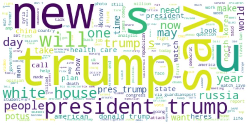
Future Internet 2021, 13, 114                                                                                             2 of 25

                                       In all of those cases, the quality of the classification model strongly depends on
                                the amount and quality of training data. Thus, gathering a suitable amount of training
                                examples is the actually challenging task. While sentiment or topic can be more easily
                                labeled, also by less experienced crowd workers [9,12], labeling a news tweet as fake or
                                non-fake news requires a lot more research, and may be a non-trivial task. For example,
                                web sites like Politifact (http://www.politifact.com/, accessed on 31 Auguest 2017), which
                                report fake news, employ a number of professional journalists for this task.
                                       In this paper, we follow a different approach. Instead of aiming at a small-scale hand-
                                labeled dataset with high-quality labels, we collect a large-scale dataset with low-quality
                                labels. More precisely, we use a different label, i.e., the trustworthiness of the source, as
                                a noisy proxy for the actual label (the tweet being fake or non-fake) This may introduce
                                false positives (since untrustworthy sources usually spread a mix of real and fake news),
                                as well as occasional false negatives (false information spread by trustworthy sources,
                                e.g., by accident), although we assume that the latter case is rather unlikely and hence
                                negligible. We show that the scarcity of hand-labeled data can be overcome by collecting
                                such a dataset, which can be done with very minimal labeling efforts. Moreover, by making
                                the data selection criteria transparent (the dataset consists of all tweets from a specified
                                set of sources over a specified time interval), we can mitigate problems of biased data
                                collection [13].
                                       In other words: we build a large scale training dataset for a slightly different task,
                                i.e., predicting the trustworthiness of a tweet’s source, rather than the truth of the tweet
                                itself. Here, we follow the notion of weakly supervised learning, more specifically, learning
                                with inaccurate supervision, as introduced by [14]. We show that a classifier trained on
                                that dataset (which, strictly speaking, is trained for classifying tweets as coming from a
                                trustworthy or a non-trustworthy source) can also achieve high-quality results on the task
                                of classifying a tweet as fake or non-fake, i.e., an F1 score of up to 0.9. Moreover, we show
                                that combining weakly supervised data with a small set of accurately labeled data brings
                                additional advantages, e.g., in the area of constructing distributional features, which need
                                larger training corpora.
                                       The rest of this paper is structured as follows. In the next section, we give an overview
                                on related work. The subsequent sections describe the dataset collection, the classification
                                approach, and an evaluation using various datasets. We close the paper with a conclusion
                                and an outlook on future work. A full description of the features used for the classification
                                is listed in an appendix. A preliminary study underlying this paper was published at
                                the IEEE/ACM International Conference on Advances in Social Networks Analysis and
                                Mining (ASONAM) [15].

                                2. Related Work
                                     Although fake news in social media is an up-to-date topic, not too much research has
                                been conducted on the automatic detection of fake news. There are, however, some works
                                which focus on a related question, i.e., assessing the credibility of tweets.
                                     Ref. [16] analyze the credibility of tweets related to high impact events using a super-
                                vised approach with a ranking support vector machine algorithm. As a training set a sample
                                of the collected data was manually annotated by three annotators (14 events×500 tweets)
                                based on related articles in well-known newspapers. Events were selected through trending
                                topics collected in a specified period. Features independently of the content of a tweet,
                                and content specific features like unigrams as well as user features were found helpful.
                                Hereby content specific features were as important as user features. It was found out that
                                the extraction of credible information from Twitter is possible with high confidence.
                                     Ref. [17] derive features for credibility based on a crowd-sourced labeling, judging,
                                and commenting of 400 news tweets. Through association rule mining, eight features were
                                identified that humans relate with credibility. Politics and breaking news were found to be
                                more difficult to rate consistently.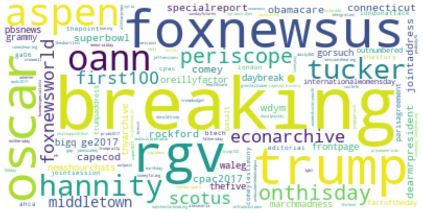
Future Internet 2021, 13, 114                                                                                             3 of 25

                                     Ref. [18] follow a different approach to assess the credibility of tweets. Three datasets
                                were collected, each related to an event. One was labeled on the basis of network activity,
                                the others were manually annotated. Two different approaches were proposed and then
                                fused in the end. On the one hand, a binary supervised machine learning classification was
                                performed. On the other hand, an unsupervised approach using expectation maximization
                                was chosen. In the latter, tweets were clustered into similar groups, i.e., claims. To that end,
                                a network was built from sources connected to their claims and vice versa. The topology
                                was then used to compute the likelihood of a claim being correct. Depending on the dataset,
                                the methods gave quite different results. Nevertheless, the fusions improved the prediction
                                error. To summarize, the supervised approach showed the better accuracy compared to the
                                expectation maximization when considering even non-verifiable tweets. However, it does
                                not predict the truthfulness of tweets.
                                     Ref. [19] also propose a supervised approach for assessing information credibility on
                                Twitter. A comprehensive set of message-, user-, topic-, and propagation-based features
                                was created. The latter refer to a propagation tree created from retweets of a message. A
                                supervised classifier was then built from a manually annotated dataset with about 600
                                tweets separated into two classes, one that states that a news tweet is almost certainly
                                true, another one for the residual. A J48 decision tree performed best within a 3-fold cross
                                validation and reached a classification accuracy of 86%. Further experiments show that a
                                subset with the propagation related features as well as a top-element subset are both very
                                relevant for the task. Thereby, the top-element subset only includes tweets with the most
                                frequent URL, hashtag, user mention, or author. However, the authors claim that user and
                                tweet features only are not sufficient to assess the credibility of a tweet.
                                     Most of these approaches share the same characteristics:
                                1.   They use datasets that are fairly small (less than 10,000 Tweets),
                                2.   they use datasets related to only a few events, and
                                3.   they rely on crowd sourcing for acquiring ground truth.
                                     The first characteristic may be problematic when using machine learning methods
                                that require larger bodies of training data. The second and the third characteristic may
                                make it difficult to update training datasets to new events, concept drift, shifts in language
                                use on Twitter (e.g., possibly changes caused by switching from 140 to 280 characters), etc.
                                     In contrast, the approach discussed in this paper acquires a dataset for the task of fake
                                news detection requires only minimal human annotation, i.e., a few lists of trustworthy
                                sources. Therefore, the process of acquiring the dataset can be repeated, gathering a
                                large-scale, up-to-date dataset at any time.
                                     As the topic of fake news detection has recently drawn some attention, there are a few
                                approaches which attempt to solve related, yet slightly different tasks, e.g., determining
                                fake news on Web pages [20–22]. Since those operate on a different type of content and
                                hence can exploit a different set of features, they are not quite comparable. Ref. [23]
                                present a descriptive study of how fake news spread on Twitter, which was able to reveal
                                characteristic patterns in the spreading of fake and non-fake news, but was not used as a
                                predictive model.

                                3. Datasets
                                     We use two datasets in this work:
                                1.   A large-scale training dataset is collected from Twitter and labeled automatically. For
                                     this dataset, we label tweets by their sources, i.e., tweets issued by accounts known to
                                     spread fake news are labeled as fake, tweets issued by accounts known as trustworthy
                                     are labeled as real.
                                2.   A smaller dataset is collected and labeled manually. This dataset is not used for
                                     training, only for validation.
                                     In the following, we describe the datasets and their collection in more detail.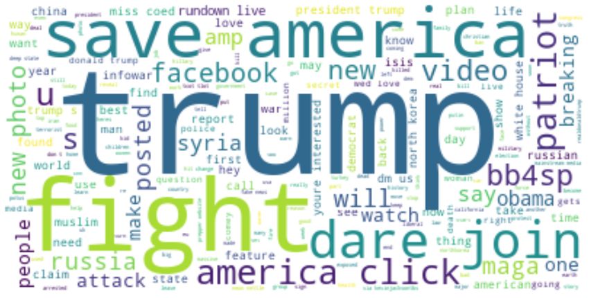
Future Internet 2021, 13, 114 4 of 25
3.1. Large-Scale Training Dataset
We create our training dataset by first collecting trustworthy and untrustworthy
sources. Then, for each of the sources, we collect Tweets using the Twitter API. Each tweet
from a trustworthy source is labeled as real news, each tweet from an untrustworthy source
is labeled as fake news.
While this labeling can be done automatically at large scale, it is far from perfect. Most
untrustworthy sources spread a mix of fake and real news. The reverse (i.e., a trustworthy
source spreading fake news, e.g., by accident) may also occur, but we assume that this case
very rare, and hence do not consider it any further.
For collecting fake news sources, we use lists from different Web pages:
• http://mashable.com/2012/04/20/twitter-parodies-news/#IdNx6sIG.Zqm (accessed
on 24 February 2017)
• https://www.dailydot.com/layer8/fake-news-sites-list-facebook/ (accessed on
24 February 2017)
• https://www.cbsnews.com/pictures/dont-get-fooled-by-these-fake-news-sites/
(accessed on 24 February 2017)
• http://fakenewswatch.com/ (accessed on 24 February 2017)
• https://www.snopes.com/2016/01/14/fake-news-sites/ (accessed on 24 February 2017)
• https://www.thoughtco.com/guide-to-fake-news-websites-3298824 (accessed on
24 February 2017)
• https://newrepublic.com/article/118013/satire-news-websites-are-cashing-gullible-
outraged-readers (accessed on 24 February 2017)
• http://www.opensources.co/ (accessed on 24 February 2017).
In total, we collected 65 sources of fake news.
For collecting trustworthy news sources, we used a copy of the recently shut down
DMOZ catalog (http://dmoztools.net/ (accessed on 25 February 2017), as well as those
news sites listed as trustworthy in opensources, and filtered the sites to those which feature an
active Twitter channel. In order to arrive at a balanced dataset, we collected 46 trustworthy
news sites. That number is incidentally chosen lower than that of fake news sources, since
we could collect more tweets from the trustworthy sites.
In the next step, we used the Twitter API (https://developer.twitter.com/en/docs
(accessed on 26 April 2021) to retrieve tweets for the sources. The dataset was collected
between February and June 2017. Since the Twitter API only returns the most recent
3200 tweets for each account (https://developer.twitter.com/en/docs/tweets/timelines/
api-reference/get-statuses-user_timeline.html (accessed on 26 April 2021), the majority
of tweets in our dataset is from the year 2017, e.g., for an active twitter account with
20 tweets per day, that limitation Twitter API allows us retrieve tweets for the past 160
days (The new Twitter API v2, which is being rolled out since the beginning of 2021, has
removed some of those limitations: https://developer.twitter.com/en/docs/twitter-api/
early-access (accessed on 26 April 2021).
In total, we collected 401,414 examples, out of which 110,787 (27.6%) are labeled as
fake news (i.e., they come from fake news sources), while 290,627 (72.4%) are labeled as real
news (i.e., they come from trustworthy sources). Figure 1 shows the distribution of tweets
by their tweet time. Due to the collection time, the maximum tweet length is 140 characters,
since the extension to 280 characters was introduced after our data collection (https://
blog.twitter.com/en_us/topics/product/2017/tweetingmadeeasier.html (accessed on 26
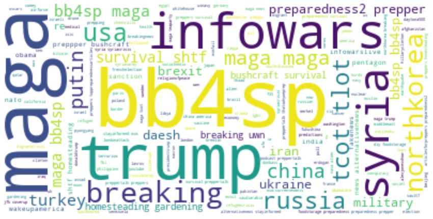
April 2021). Figure 2 shows the topical distribution of the tweets. Figure 3 depicts further
statistics about the tweets in the training set. It can be observed that while there is no
strong difference in the sentiment (average 0.39 on the real class, 0.38 on the fake class) and
the subjectivity score (average 0.27 on the real class, 0.29 on the fake class), the number of
retweets (average 123 on the real class, 23 on the fake class) and favorites (average 236 on
the real class, 34 on the fake class) differ considerably.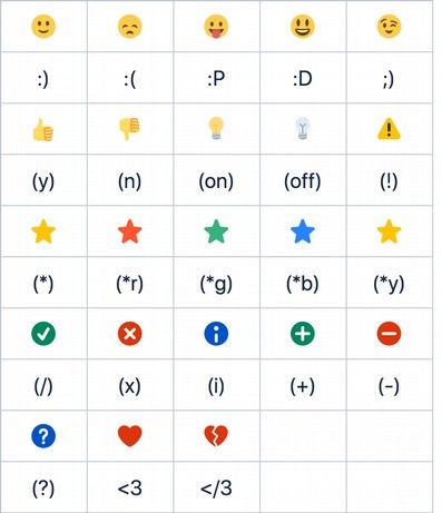
Future Internet 2021, 13, 114                                                                                                           5 of 25

                                                       Fake
                                            60000      Real

                                            50000

                                            40000
                                # of news
                                            30000

                                            20000

                                            10000

                                               0
                                                    1-15 3-15 5-15 7-15 9-15 11-15 1-16 3-16 5-16 7-16 9-16 11-16 1-17 3-17 5-17
                                                                                        Month

                                Figure 1. Distribution of tweets labeled as real and fake news in the training dataset.

                                (a) Word cloud of the real news class                           (b) Word cloud of the fake news class

                                (c) Tag cloud of the real news class                            (d) Tag cloud of the fake news class

                                Figure 2. Topic distribution in the training dataset.

                                     It is important to point out that for collecting more than 400 k tweets, the actual annota-
                                tion workload was only to manually identify 111 sources. In other words, from 111 human
                                annotations (trustworthy vs. untrustworthy source), we produce 400 k annotated tweets.
                                     As discussed above, we expect the real news class to contain only a negligible amount
                                of noise, but we inspected the fake news class more closely. The results are depicted in
                                Table 1. The fake news class contains a number of actual news (a phenomenon also known
                                as mixed information [24]), as well as tweets which are not news, but other contents (marked
                                as “no news” in the table). These numbers show that the fake news tweets are actually the
                                smallest class in the training sample. However, since the sample contains both real and
                                fake news tweets from the same period of time, we can assume that for real news, those
                                will also appear in the class labeled as non-fake, and since the real news class is larger by a
                                factor of three, the classifier will more likely label them as real news. For example, if a real
                                news item is tweeted by eight real and two fake news sources, a decent classifier would, to
                                put it very simply, learn that it is a real news item with 80% confidence. This shows that
                                the incidental imbalance of the dataset towards real news is actually useful.
Future Internet 2021, 13, 114                                                                                                   6 of 25

                                (a) Sentiment score                                   (b) Subjectivity score

                                (c) Retweet count                                     (d) Favorite count

                                Figure 3. Statistics on sentiment and subjectivity score, as well as on retweet and favorite counts.

                                Table 1. Actual distribution of tweets in the sample drawn from sources known to contain fake news.

                                                      Category                                          Amount
                                                      Fake news                                          15.0%
                                                      Real news                                          40.0%
                                                       No news                                           26.7%
                                                       Unclear                                           18.3%

                                3.2. Small-Scale Evaluation Dataset
                                       For creating a hand-labeled gold standard, we used 116 tweets from the politifact web
                                site that were classified as fake news by expert journalists (see above). Those were used
                                as positive examples for fake news tweets. Note that the sources of those tweets are not
                                sources that have been used in the training set. For generating negative examples, and in
                                order to arrive at a non-trivial classification problem, we picked those 116 tweets which
                                were the closest to the fake news tweets in the trustworthy class according to TF-IDF and
                                cosine similarity. By this, we created a balanced gold standard for evaluation of 232 tweets
                                classified as real and fake news.
                                       The rationale for this approach instead of using explicit real news (e.g., from politifact)
                                is not to overly simplify the problem. By selecting a random set of real and fake news each,
                                it is likely to end up with topically unrelated tweets, also since fake news do not spread
                                equally across all news topics. In that case, a classifier could simply learn to distinguish the
                                topics instead of distinguishing fake from real news.
                                       In order to eliminate overfitting effects, we removed the 116 tweets used as negative
                                examples from the training dataset before training our classification models.
Future Internet 2021, 13, 114                                                                                              7 of 25

                                3.3. Evaluation Scenarios
                                     We consider two different evaluation scenarios. Scenario 1 only considers the tweet as
                                such. Here, we examine the case where we have a tweet issued from an account for which
                                there is no additional information, e.g., a newly created account.
                                     Scenario 2 also includes information about the user account from which the tweet was
                                sent. Since including as much information as possible will likely improve the results, we
                                expect the mere results of Scenario 2 to be better than those in scenario 1. However, the
                                Scenario 2 is only applicable for user accounts that have been active for a certain period of
                                time, whereas Scenario 1 has no such constraints.

                                4. Approach
                                     We model the problem as a binary classification problem. Our approach is trained on
                                the large-scale, noisy dataset, using different machine learning algorithms. All of those
                                methods expect the representation of a tweet as a vector of features. Therefore, we use
                                different methods of extracting features from a tweet. We consider five different groups of
                                features: user-level features, tweet-level features, text features, topic features, and sentiment
                                features. For the feature engineering, we draw from previous works that extract features
                                from tweets for various purposes [7,16,18,19,25–28].
                                     The overall approach is depicted in Figure 4. A human expert labels a list of sources,
                                which are then used to crawl tweets for those sources. These crawled tweets then serve as
                                input to a machine learning classifier as examples labeled by weak supervision, and are
                                enriched by different feature generation strategies.

                                                                      provides

                                                     Annotated List                Expert
                                                       of Sources

                                                                                  List of Weakly
                                                                                 Annotated Tweets   Machine Learning
                                Twitter API                                                              Model
                                                    Twitter Crawler

                                                                                 Feature Creation

                                Figure 4. Schematic depiction of the overall approach.

                                4.1. User-Level Features
                                      For the user, we first collect all features that the Twitter API (https://developer.twitter.
                                com/en/docs/api-reference-index, accessed on 26 April 2021) directly returns for a user,
                                e.g., the numbers of tweets, followers, and followees, as well as whether the account is a
                                verified account or not (see https://help.twitter.com/en/managing-your-account/about-
                                twitter-verified-accounts, accessed on 26 April 2021).
                                      In addition to the user-level features that can be directly obtained from the Twitter
                                API, we create a number of additional features, including:
                                •     Features derived from the tweet time (e.g., day, month, weekday, time of day);
                                •     features derived from the user’s description, such as its length, usage of URLs, hash-
                                      tags, etc.;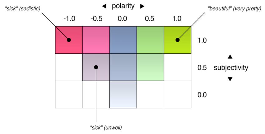
Future Internet 2021, 13, 114                                                                                          8 of 25

                                •    features derived from the user’s network, e.g., ratio of friends and followers;
                                •    features describing the tweet activity, such as tweet, retweet, and quote frequency,
                                     number of replies, and mentions, etc.;
                                •    features describing the user’s typical tweets, such as ratio of tweets containing hash-
                                     tags, user mentions, or URLs.
                                     In total, we create 53 user-level features. Those are depicted in Tables A1 and A2 in
                                the Appendix A.

                                4.2. Tweet-Level Features
                                     For tweet-level features, we again first collect all information directly available from
                                the API, e.g., number of retweets and retweets, as well as whether the tweet was reported
                                to be sensitive (see https://help.twitter.com/en/safety-and-security/sensitive-media,
                                accessed on 26 April 2021).
                                     In addition, we create a number of additional features characterizing a tweet, e.g.,
                                •    features characterizing the tweet’s contents, such as URLs, hashtags, user mentions,
                                     and emojis. For emojis, we also distinguish face positive, face negative, and face
                                     neutral emojis (http://unicode.org/emoji/charts/full-emoji-list.html, accessed on
                                     20 May 2017, and http://datagenetics.com/blog/october52012/index.html, accessed
                                     on 9 May 2017);
                                •    features characterizing the tweet’s language, such as punctuation characters, character
                                     repetitions, and ratio of uppercase letters;
                                •    linguistic features, such as ratio of nouns, verbs, and adjectives (using WordNet [29]
                                     and NLTK [30], number of slang words, determined using Webopedia (http://www.
                                     webopedia.com/quick_ref/Twitter_Dictionary_Guide.asp, accessed on 27 April 2021)
                                     and noslang.com (http://www.noslang.com/dictionary/, accessed on 27 April 2021),
                                     and existence of spelling mistakes (determined using the pyenchant (https://pypi.org/
                                     project/pyenchant/, accessed on 28 April 2021) library).
                                     In total, we create 69 tweet-level features. The full list of features is depicted in
                                Tables A3 and A4. In order to make the approach applicable in real-time scenarios and
                                be able to immediately classify new tweets, we remove time-dependent attributes (i.e.,
                                number of retweets and number of favorites).

                                4.3. Text Features
                                     The features above do not consider the actual contents of the tweet. For representing
                                the textual contents of the tweet, we explored two alternatives: a bag of words (BOW)
                                model using TF-IDF vectors, and a neural Doc2vec model [31] trained on the corpus. For
                                the BOW approach, we explored the use both of word unigrams and word bigrams. The
                                results of an initial experiment using different learners in their default configuration, and
                                running cross validation on the training set, are depicted in Table 2. It can be observed
                                that unigrams work better than bigrams for BOW models, most likely due to the high
                                dimensionality of the latter.
Future Internet 2021, 13, 114 9 of 25
Table 2. The performances of the learners with a bag-of-words model with 500 terms for unigrams
and 250 terms for bigrams. The best performance for unigrams and biagrams is marked in bold.
Learner Variant Precision Recall F1-Measure
Naive Bayes unigram 0.3943 0.6376 0.4873
Decision Tree unigram 0.4219 0.4168 0.4193
SVM unigram 0.5878 0.1559 0.2465
Neural Network unigram 0.4471 0.3951 0.4195
XGBoost unigram 0.6630 0.0641 0.1170
Random Forest unigram 0.5226 0.4095 0.4592
Naive Bayes bigram 0.4486 0.1320 0.2040
Decision Tree bigram 0.4139 0.3178 0.3595
SVM bigram 0.5930 0.1029 0.1754
Neural Network bigram 0.3935 0.1414 0.2081
XGBoost bigram 0.4083 0.0596 0.1040
Random Forest bigram 0.4450 0.2945 0.3544
For doc2vec, two variants exist. On the one hand, the Continuous Bag-of-words
model (CBOW) predicting a word at hand based on its context. The context is represented
in a bag-of-words fashion, thus the order of the words is not considered. On the other
hand, the Continuous Skip-gram model which predicts the surrounding words given a
word [32]. Doc2Vec does not only use word vectors, but also paragraph vectors which
represent a text of arbitrary length rather than single words. Word vectors are shared
across paragraphs whereas paragraph vectors are only shared across the contexts within a
paragraph. With Doc2Vec, it is possible to represent texts of variable length with a vector
of a fixed size which is usually much smaller than the vocabulary size. This vector can
then be used as features for tasks requiring a two dimensional text representation like
the one in this paper. Again, two frameworks can be applied to achieve the vectors. The
Distributed Memory Model (PV-DM) is similar to CBOW, but also includes a paragraph
matrix in addition to the word vectors which then are used to predict a word in the context.
Similar to the skip-gram model for Word2Vec, the Distributed Bag-of-words for paragraph
vectors (PV-DBOW) predicts words from a small window given the paragraph matrix.
The order of the words in this window is not considered [31]. The Python library gensim
(https://radimrehurek.com/gensim/, accessed on 7 June 2017) was used to create the
vectors. As an input for Doc2Vec, preprocessing stage five was considered. This stage
also includes stopwords. However, Doc2Vec is able to handle them through the sample
parameter, which randomly downsamples higher-frequency words (https://radimrehurek.
com/gensim/models/doc2vec.html, accessed on 7 June 2017).
While the BOW model yields a fixed number of features (since each possible word
in the corpus is regarded as a single feature), we can directly influence the number of
features created by Doc2vec. We have experimented with 100, 200, and 300 dimensions,
training the model using the gensim Python library (https://radimrehurek.com/gensim/,
accessed on 7 June 2017), and using both the Distributed Memory (DM) and the Distributed
Bag of Words (DBOW) variant. In an initial experiment, running cross validation on
the training set, DBOW constantly outperformed DM, but the number of dimensions for
which the best results were achieved varied across the learning algorithms, as depicted
in Figure 5. Comparing the results to those obtained with BOW above, we can observe
that doc2vec yields superior results. Hence, we used doc2vec for text representation in
the subsequent experiments, using the best performing configuration for each learning
algorithm from the initial experiments (Interaction effects of the parameter settings for
doc2vec and the learning algorithm were not analyzed due to the size of the combined
parameter search space).Future Internet 2021, 13, 114 10 of 25
GaussianNB DecisionTreeClassifier
0.425
0.55
F1-measure
F1-measure
0.400
0.50
0.375
0.45 0.350
100 200 300 100 200 300
Vector Size Vector Size
0.60
MLPClassifier LinearSVC
F1-measure
F1-measure
0.5
0.55
0.4
0.50
100 200 300 100 200 300
Vector Size Vector Size
XGBClassifier RandomForestClassifier
0.45 0.325
F1-measure
F1-measure 0.300
0.40
0.275
0.35
0.250
0.30
100 200 300 100 200 300
Vector Size Vector Size
DBOW DM
Figure 5. F1 scores using different dimensions for Doc2vec, using DBOW (in blue) and DM (in red).
4.4. Topic Features
Since the topic of a tweet may have a direct influence on the fake news classification, as
some topics are likely more prone to fake news than others, we also apply topic modeling
for creating features from the tweets. Again, we train topic models using the gensim library.
Latent Dirichlet Allocation (LDA) is a three-level hierarchical Bayesian model of a set of
documents. Each document is modeled as a mixture of a set of K topics. In turn, each topic
is modeled through a distribution over words [33]. The number of topics, i.e., K, is a user
defined number. In a nutshell, the algorithm first assigns a random topic to each word in
the corpus and then iteratively improves these guesses based on the probability for a topic,
given a word and a document until a convergence criteria is met. As a simplified example,
assume that LDA was configured to discover two topics t0 and t1 from ten documents,
i.e., K = 2. The output of LDA is then, for instance, that the first document is 80% about
topic t0 , whereas another document is 40% about t0 and 40% about topic t1 . These topics t0
and t1 are then in turn built from words in the documents. For example, topic t0 is built
50% from a word w0 , 30% from a word w1 and so on. The LDA implementation for online
learning was similar to Doc2Vec chosen from the gensim library. The advantage of using an
online instead of a batch implementation is that documents can be processed as a stream
and discarded after one look. Hence, documents do not need to be stored locally, which in
turn is memory efficient [34].
One of the major disadvantages of LDA is that K, i.e., the number of topics is a
mandatory user specified parameter. Especially when a fixed number of topics is hard
to determine as it is for news tweets, setting the best value is not an easy task. The
Hierarchical Dirichlet Process (HDP) proposed by [35] solves this problem. It is used to
generalize LDA and determines the number of clusters directly from the data. In LDA, a
topic is represented by a probability distribution across a set of words and a document by
a probability distribution across a finite set of topics. In the nonparametric version, alsoFuture Internet 2021, 13, 114 11 of 25
referred to as HDP-LDA, the topics do not come from a finite set but they are linked, so that
the same topic can appear in different documents [36]. Again, the online implementation
from the gensim library was used. It is inspired by the one for LDA and thus provides the
same benefits. In previous research, it has been demonstrated on two text collections that
the HDP outperforms the online LDA model according to the per-word likelihood [37].
We trained both a Latent Dirichlet Allocation model (LDA) on the whole dataset,
varying the number of topics between 10 and 200 in steps of 10, as well as a Hierar-
chical Dirichlet Process (HDP) model. As for the text representations with BOW and
doc2vec, we conducted a prestudy with different classifiers in their standard configura-
tions, and cross validation on the training set. As shown in Figure 6, LDA constantly
outperformed HDP, but the number of topics at which the best results are achieved again
varies between learners.
GaussianNB LinearSVC
0.40
0.35 0.2
F1-measure
F1-measure
0.30 0.1
0.25
0.20 0.0
0 50 100 150 200 0 50 100 150 200
Number of Topics Number of Topics
MLPClassifier XGBClassifier
0.4 0.3
F1-measure
F1-measure
0.3 0.2
0.1
0.2
0.0
0 50 100 150 200 0 50 100 150 200
Number of Topics Number of Topics
DecisionTreeClassifier RandomForestClassifier
0.400 0.35
F1-measure
F1-measure
0.375
0.350 0.30
0.325
0.300 0.25
0 50 100 150 200 0 50 100 150 200
Number of Topics Number of Topics
Figure 6. F1 scores using different numbers of topics for LDA with different learning algorithms (in
blue), and the results for HDP (in red).
4.5. Sentiment Features
The polarity of a tweet can be assessed in terms of positivity, neutrality, or negativity.
Additionally, a lemmatization was performed to get a base form of the words. The meaning
of words depend on the semantic of the sentence, and thus the context. Hence, the first step
was to identify this meaning. In NLP, this task is called Word Sense Disambiguation. One of
the most popular algorithms for the disambiguation of word senses is the Lesk algorithm.
This algorithm uses word dictionaries with explanations for each word’s sense. Words from
the sense definition are then crosschecked for overlaps with words in the sense definition
of the other words in context. The sense with the highest overlap is then chosen for each
word in context [38]. In the NLTK implementation, which was used in this paper, WordNet
is used as a dictionary. In that implementation, part-of-speech tags can be included for
disambiguation as well. To determine the sentiment of a tweet, SentiWordNet was thenFuture Internet 2021, 13, 114 12 of 25
used to get a positive and negative score for every single word in the context. SentiWordNet
is a publicly available lexicon with the annotation of all synsets in WordNet according to
their positivity, negativity, and neutrality [39]. All nouns, verbs, adjectives, and adverbs
were evaluated, and the difference of positive and negative sentiment was calculated as a
sentiment score for each word.
On Twitter, sentiment is not only expressed in words, but also by using emoticons.
At this point, emoticons have not yet been considered. Therefore, an emoticon dictionary
for Unicode emojis [40], as well as one for ASCII emoticons [41], were used here to look
up the sentiment of the emoticons. After all tokens in the sentence have been scored, the
tweet’s score was calculated by summing up the individual scores. Through summing
up the sentiments, the sum’s lower and upper bound is limited by the number of words
in a tweet, and thus the 140 character limitation. In a tweet with 20 sentiment words of
which all are positive, i.e., each word has a score of +1, the sentiment sum would be 20. If
in another tweet there is only one positive word, the sum would be much lower. It is clear
that in this example the tweet with more sentiment words also gets higher scores even if
both are completely positive. Therefore the sum was divided by the number of sentiment
words in the tweet to get the average sentiment score. Sentiment is usually given in a range
of −1 to 1. However, since many machine learning classifiers operate better on features in
a [0, 1] interval, the sentiment score was normalized to a range from 0 to 1, i.e., tweets with
a score of 0.5 are completely neutral.
In addition to the previous approach, an implementation from the TextBlob (http:
//textblob.readthedocs.io/en/dev/index.html, accessed on 27 April 2021) library was also
considered. This implementation is a lexicon approach as well. It is based on the web
mining module Pattern, which was proposed by [42]. Compared to SentiWordNet, Pattern
does not only provide scores for polarity, but also a degree of subjectivity. Polarity scores
span from −1, which is very negative, to 1, which is very positive. Objective words get a
score of 0, whereas highly subjective words like handsome get a score of 1. In Pattern, words
were manually annotated based on the triangle representation, which is shown in Figure 7.
The authors claim that “[...] more positive/negative adjectives are also more subjective [but]
not all subjective adjectives are necessarily positive or negative [...]” [43]. Although the
paper is primarily about Dutch language, the proposed English word annotation showed
good results on their test data, too. Unfortunately, the dictionary only scores words, and
thus does not include emoticons. Nevertheless, the TextBlob implementation was used as an
estimator for subjectivity. URLs, user mentions, hashtags, and punctuation were removed
and the remaining text was passed on to the library which then returned a subjectivity
score for the text. The tweet feature called subjectivity_score refers to this value.
Figure 7. Representation of polarity and subjectivity scores by [43].
Polarity and subjectivity scores account for eight additional features. Table A5 in the
Appendix A gives an overview of those features.
4.6. Feature Scaling and Selection
The resulting feature set combining all of the above strategies is fairly large, hence, we
expect performance gains from dimensionality reduction or feature selection. We exploredFuture Internet 2021, 13, 114 13 of 25
three different options here: setting a minimum variance threshold, recursive elimination
using the Gini index as an importance criterion, and recursive elimination using mutual
information [44]. The first removes all features which do not have a minimum variance
(in our experiments, we used a minimum variance of 0.005), the latter two recursively
eliminate the lowest ranked features according to the respective importance measure until
the performance drops.
For machine learning approaches that are sensitive to scales, such as Support Vector
Machines, we standardize all features first, using a z-transformation in a preprocessing step.
4.7. Learning Algorithms and Parameter Optimization
As learning algorithms, we use Naive Bayes, Decision Trees, Support Vector Machines
(SVM), and feed-forward Neural Networks as basic classifiers. Moreover, we use two
ensemble methods known to usually work well, i.e., Random Forest and XGBoost, as well
as voting among all of those methods in two flavors (simple majority voting, and weighted
voting based on the classifiers’ confidences).
While Naive Bayes and Decision Trees were used in their standard configuration, we
performed some parameter optimization for the other classifiers, using a 10% stratified
sample of our training dataset. For SVM, we optimized the parameters C and γ as described
by [45]. For Neural Networks, we follow the observation by [46] that one hidden layer is
sufficient for most classification problems. We optimized the number of neurons in the
hidden layer along with many other parameters, such as activation function, learning rate,
regularization penalty, and the maximum number of training epochs, using random search
as suggested by [47]. Finally, for Random Forests and XGBoost, we pick the number of
trees to be learned by simple grid search.
5. Evaluation
We evaluate our approach in different settings. First, we perform cross-validation
on our noisy training set; second, and more importantly, we train models on the training
set and validate them against a manually created gold standard (The code and data are
available at https://github.com/s-helm/TwitterFakeNews (accessed on 27 April 2021).
Moreover, we evaluate two variants, i.e., including and excluding user features. The
rationale of the latter is to simulate two use cases: assessing a tweet from a known user
account, and assessing a tweet from a new user account.
In order to further analyze the benefit of our dataset, we also run a cross validation
on the evaluation set, and we explore how distributional features generated by utilizing a
large-scale dataset (in particular: text and topic features) can be injected into a clean, but
smaller training set.
Since the original training set was labeled by source, not by tweet, the first setting
evaluates how well the approach performs on the task of identifying fake news sources,
whereas the second setting evaluates how well the approach performs on the task of
identifying fake news tweets—which was the overall goal of this work. It is important
to note that the fake news tweets come from sources that have not been used in the
training dataset.
5.1. Setting 1: Cross-Validation on Training Dataset
To analyze the capabilities of the predictive models trained, we first perform cross-
validation on the training dataset. Due to the noisy nature of the dataset, the test dataset
also carries noisy labels with the same characteristics as the training dataset, and thus, we
expect the results to over-estimate the actual performance on a correctly labeled training
dataset. Hence, the results depict an upper bound of our proposed weak supervision method.
The results are shown in Tables 3 and 4. Not surprisingly, adding information on
the user clearly improves the results. We can observe that the best results are achieved
using XGBoost, leading to an F1 score on the fake news class of 0.78 and 0.94, respectively.Future Internet 2021, 13, 114 14 of 25
Although voting using all base classifiers improves over the results of XGBoost alone, the
improvement is rather marginal.
Table 3. Cross validation results with tweet features only, and number of features used (#F). Abbre-
viations: Learners—Naive Bayes (NB), Decision Tree (DT), Neural Network (NN), Support Vector
Machine (SVM), XGBoost (XGB), Random Forest (RF); Feature Selection (FS), Voting (V), Weighted
Voting (WV)—Variance Threshold (V), Recursive Elimination with Mutual Information (MI) and
with Gini Index (G). The best results are marked in bold.
Learner #F FS Prec. Rec. F1
NB 409 V 0.7024 0.6080 0.6518
DT 845 – 0.6918 0.6401 0.6649
NN 463 MI 0.8428 0.6949 0.7618
SVM 565 MI 0.8492 0.6641 0.7453
XGB 106 G 0.8672 0.7018 0.7758
RF 873 G 0.8382 0.6494 0.7318
V – – 0.8650 0.7034 0.7759
WV – – 0.8682 0.7039 0.7775
Table 4. Cross validation results with tweet and user features. The best results are marked in bold.
Learner #F FS Prec. Rec. F1
NB 614 V 0.8704 0.8851 0.8777
DT 34 G 0.8814 0.9334 0.9067
NN 372 V 0.8752 0.8861 0.8806
SVM 595 MI 0.9315 0.7727 0.8447
XGB 8 G 0.8946 0.9589 0.9256
RF 790 G 0.8923 0.8291 0.8596
V – – 0.9305 0.9416 0.9360
WV – – 0.9274 0.9384 0.9329
5.2. Setting 2: Validation Against Gold Standard
As discussed above, the more important setting validates the approach using a manu-
ally annotated gold standard. Since that gold standard dataset was collected independently
from the training dataset, and is never used for training, feature selection, or parameter
optimization, we can safely state that our approach is not overfit to that dataset.
For the feature sets, feature selection methods, and parameter settings, we used the
setups that worked best in the cross validation settings. More precisely, the feature sets
and feature selection methods are those depicted in Tables 3 and 4.
The results of that evaluation are shown in Tables 5 and 6. In contrast to the results
in cross validation, the neural network learner performs best in that scenario, and voting
across all learners does not improve the results.Future Internet 2021, 13, 114 15 of 25
Table 5. Results on manually labeled gold standard, using tweet features only. The best results are
marked in bold.
Learner Precision Recall F1-Measure
NB 0.6835 0.4655 0.5538
DT 0.7895 0.6466 0.7109
NN 0.7909 0.7500 0.7699
SVM 0.7961 0.7069 0.7489
XGB 0.8333 0.6897 0.7547
RF 0.8721 0.6466 0.7426
V 0.8200 0.7069 0.7593
WV 0.8478 0.6724 0.7500
Table 6. Results on manually labeled gold standard, using both tweet and user features. The best
results are marked in bold.
Learner Precision Recall F1-Measure
NB 0.8333 0.9052 0.8678
DT 0.8721 0.6466 0.7426
NN 0.9115 0.8879 0.8996
SVM 0.8942 0.8017 0.8455
XGB 0.8679 0.7931 0.8288
RF 0.8713 0.7586 0.8111
V 0.8870 0.8793 0.8831
WV 0.8761 0.8534 0.8646
Table 7 summarizes the best achieved results for each of the four settings. It is
remarkable that the results are not much worse than those achieved in cross validation:
with tweet features only, the best F1 score achieved is 0.77 (compared to 0.78), with both
tweet and user features, the best F1 score is 0.90 (compared to 0.94). This proves that our
approach of using a large-scale, noisy training dataset is actually valid and yields results
of remarkable quality, even though the classifier employed was originally trained on a
different task.
Table 7. Results summary, depicting the best F1 score achieved for each task (fake news source and
fake news tweet detection), as well as for each feature group (tweet level features only and tweet and
source features).
Identifying Fake News...
Sources Tweets
Tweet features only 0.7775 (Table 3) 0.7699 (Table 5)
Tweet and user features 0.9360 (Table 4) 0.8996 (Table 6)
5.3. Comparison to Training on Manually Labeled Data
In order to be able to better judge the results above, we also ran a set of experiment
where we use cross validation on the evaluation set, i.e., we use the manually labeled data
as training signal. The goal of this experiment is to analyze how close the quality using
weak supervision would get to results achieved through human expert labeling, which is
expected to yield superior results.Future Internet 2021, 13, 114 16 of 25
Here, we distinguish two cases:
1. In the first setup, we have re-created all content features for the manually labeled
dataset (On the manually labeled dataset, LDA was not able to generate meaningful
results due to the very small dataset size. Hence, we have left out the LDA based
features in the first setup).
2. In the second setup, we used the distributional text and topic features (doc2vec, LDA)
created from the weakly supervised set.
The latter case can be considered a combined setup, where information from the
large dataset obtained through weak supervision was used to improve the results on the
manually labeled dataset.
The parameter settings were the same as in the experiments on the large-scale training
data. The results are depicted in Tables 8 and 9. They show that the F1 scores are in the same
range when using the manually labeled tweets as when using the ones labeled through
weak supervision—when using tweet features only, training on the manually labeled data
works slightly better, when using all features, training on the weak supervision set works
slightly better. This supports our claim that our methodology for generating training
data is valid in the sense that it yields datasets of comparable quality in downstream
classification tasks.
Table 8. Cross validation results on manually labeled gold standard, using tweet features only. We
distinguish a setup with re-created features for the manually labeled dataset, and re-using features
from the large dataset. The best results are marked in bold.
Re-Created Features Features from Large Set
Learner Precision Recall F1-Measure Precision Recall F1-Measure
NB 0.5912 0.6983 0.6403 0.4425 0.4310 0.4367
DT 0.6944 0.6466 0.6696 0.7156 0.6724 0.6933
NN 0.7500 0.8017 0.7750 0.6640 0.7155 0.6888
SVM 0.7311 0.7500 0.7404 0.8585 0.7845 0.8198
XGB 0.8000 0.7586 0.7788 0.7797 0.7931 0.7863
RF 0.7524 0.6810 0.7149 0.7938 0.6638 0.7230
Table 9. Cross validation results on manually labeled gold standard, using user and tweet features.
We distinguish a setup with re-created features for the manually labeled dataset, and re-using features
from the large dataset. The best results are marked in bold.
Re-Created Features Features from Large Set
Learner Precision Recall F1-Measure Precision Recall F1-Measure
NB 0.8235 0.7241 0.7706 0.5619 0.6983 0.6255
DT 0.8750 0.9052 0.8898 0.8571 0.8793 0.8681
NN 0.8547 0.8621 0.8584 0.8110 0.8879 0.8477
SVM 0.8584 0.8362 0.8472 0.9299 0.9138 0.9217
XGB 0.8947 0.8793 0.8870 0.8983 0.9138 0.9059
RF 0.8618 0.9138 0.8870 0.8522 0.8448 0.8485
In our second setup, we use the distributional features created on the large-scale
dataset. Here, our intuition is that approaches such as LDA and doc2vec yield good results
only when trained on larger corpora. When using those features for classification with the
manually labeled data, we obtain the best results overall, surpassing both the setup with
manually labeled data only and the setup with labeling through weak supervision only by
3–4 percentage points in F1 score.Future Internet 2021, 13, 114 17 of 25
5.4. Feature Importance
Another question we look into is the relative importance of each feature for the task
of fake news detection. Since XGBoost can also compute an importance score for each
feature, we could directly plot the most relevant features for the two evaluation scenarios,
as depicted in Figures 8 and 9.
Relative Feature Importance
tweet__nr_of_hashtags 0.0799999981559813
tweet__ratio_capitalized_words 0.06428571785966467
tweet__contains_character_repetitions 0.04857143011276743
tweet__ratio_uppercase_letters 0.04857143011276743
tweet__text_length 0.04571428519274507
tweet__nr_of_urls 0.03714285788325859
tweet__nr_of_exclamation_marks 0.02857142871112696
tweet__month_of_year 0.02571428565374975
tweet__ratio_stopwords 0.02571428565374975
tweet__nr_of_user_mentions 0.024285715056383717
tweet__truncated 0.024285715056383717
tweet__contains_pronouns 0.021428571999006506
tweet__d2v_219 0.019999999538995325
tweet__day_of_month 0.017142856481618115
tweet__nr_of_words 0.015714285884252083
tweet__d2v_117 0.01428571435556348
tweet__d2v_4 0.01428571435556348
tweet__contains_quote 0.01428571435556348
tweet__d2v_225 0.012857142826874874
tweet__d2v_201 0.012857142826874874
0.00 0.03 0.06 0.09 0.12 0.15 0.18 0.21 0.24 0.27
Relative Importance
Figure 8. Feature importance for Scenario 1 (tweet level features only), as computed by XGBoost.
Relative Feature Importance
user__listed_count 0.26293104397261435
user__avg_time_between_tweets 0.15301723493231023
user__created_days_ago 0.15086206512782602
user__percent_with_url 0.14439655571437338
user__max_time_between_tweets 0.08405171923243032
tweet__month_of_year 0.0797413796234619
user__geo_enabled 0.0668103458953957
user__favourites_count 0.058189655501588146
0.00 0.05 0.10 0.15 0.20 0.25 0.30 0.35 0.40 0.45
Relative Importance
Figure 9. Feature importance for Scenario 2 (tweet and user level features), as computed by XGBoost.
The first observation to be made is that user features, if made available as in Scenario 2,
receive a much higher weight. The explanation for this is two fold: first, it is an effect of the
specific type of weak supervision used, since the original labels are labels for tweet sources,
and each tweet source corresponds to a Twitter user. Second, there is obviously a strong
correlation between user behavior (e.g., tweet frequency, usage of URLs) and the likelihoodFuture Internet 2021, 13, 114 18 of 25
of a tweet being fake news. The network of a user also matters: the strongest indicator is
the containment of a user in lists created by other users.
When looking at tweet level features only, as in Scenario 1, more features with lower
weights are selected by XGBoost, indicating that this classification problem is inherently
harder. We can see that text surface features, such as capitalization, character repetitions,
and exclamation marks play a more crucial role in this respect. Moreover, quite a few
doc2vec features for the contents are selected, while topics and sentiment features are not
considered helpful by XGBoost.
The fact that the month of the year is selected as a relevant feature is probably an
artifact of the dataset distribution, as shown in Figure 1. From this distribution, we can see
that the months February–June 2017 have a higher ratio of real to fake news tweets than
the other months, which is an effect of the data collection and the rate limitations of the
Twitter API, as discussed above.
6. Conclusions and Outlook
In this work, we have shown a practical approach for treating the identification of
fake news on Twitter as a binary machine learning problem. While that translation to a
machine learning problem is rather straight forward, the main challenge is to gather a
training dataset of suitable size. Here, we have shown that, instead of creating a small,
but accurate hand-labeled dataset, using a large-scale dataset with inaccurate labels yields
competitive results.
The advantages of using our approach are two-fold. First, the efforts for creating
the dataset are rather minimal, requiring only a few seed lists of trustworthy and non-
trustworthy Twitter accounts, which exist on the Web. Second, since the dataset is can be
created automatically to a large extent, it can updated at any point of time, thus accounting
for recent topics and trends, as well as changes in the social media service (e.g., the change
from 140 to 280 characters in Twitter, or the availability of different content via changes
in the API (https://developer.twitter.com/en/docs/twitter-api/early-access, accessed
on 27 April 2021). In contrast, a hand-labeled dataset might lose its value over time for
those reasons. In a practical setup, a fake news detection system based on our approach
could continuously collect training data and periodically update its classification models.
Moreover, it would allow broadening the scope of the work—while in this work, we have
mainly considered political fake news, we could take the same approach to also detect fake
news in other domains. Topic classification of tweets would be possible with a similar
approach as well—since there are quite a few Twitter accounts which are mainly focused on
a particular topic, a training dataset for that task could be sourced with the same approach.
We have shown that our approach yields very good results, achieving an F1 score of
0.77 when only taking into account a tweet as such, and up to 0.9 when also including
information about the user account. It is particularly remarkable that the results are not
much worse than those achieved for classifying trustworthy and untrustworthy sources
(which is actually reflected in the labels for the tweets): with tweet features only, the best
F1 score achieved is 0.78, with both tweet and user features, the best F1 score 0.94.
To date, we have used features based on the tweets and user accounts, but there are
other alternatives as well. For example, for tweets containing a URL, we are currently
not collecting any information from and about that URL. The same holds for images and
other media in tweets. Second, we only record the number of retweets and likes of a tweet,
but do not analyze comments and answers to a tweet, nor any information derived from
the user accounts that retweeted a tweet. However, our feature analysis has revealed that
the network of users (as manifested, e.g., in the number of user created lists an account
is contained in) plays an important role for the classification task at hand. Here, stepping
from the level of tweets and users as single entities to considering the entire network of
users and tweets would yield new opportunities.
From a machine learning perspective, we have so far taken well-known classification
approaches, and shown that they can be applied even in our setting, where the labelFuture Internet 2021, 13, 114 19 of 25
information is noisy (more precisely: where one class is particularly prone to noise). There
are quite a few works which theoretically examine the effect of label noise on the learning
algorithms and propose specific methods for tailoring learning algorithms for those cases,
as well as for cleansing label noise as a preprocessing step [48–50]. Further exploring the
application of such techniques will be an interesting aspect of future work in this direction.
In summary, we have shown that the problem of acquiring large-scale training datasets
for fake news classification can be circumvented when accepting a certain amount of label
noise, which can be used to learn classification models of competitive performance.
Author Contributions: Conceptualization, H.P. and S.H.; methodology, H.P. and S.H.; software, S.H.;
validation, H.P. and S.H.; formal analysis, H.P.; investigation, S.H.; resources, S.H.; data curation,
S.H.; writing—original draft preparation, S.H.; writing—review and editing, H.P.; visualization, H.P.;
supervision, H.P.; project administration, H.P. All authors have read and agreed to the published
version of the manuscript.
Funding: This research received no external funding.
Institutional Review Board Statement: Not applicable.
Informed Consent Statement: Not applicable.
Data Availability Statement: Data is available at https://github.com/s-helm/TwitterFakeNews
(accessed on 26 April 2021).
Conflicts of Interest: The authors declare no conflict of interest.
Appendix A. Features
Appendix A.1. User-Level Features
Table A1. Overview of the attributes of a user returned by the Twitter API.
Feature Name Description
default_profile Indicates that a user has not changed the theme or background
favourites_count The number of tweets the user liked at the point of gathering
followers_count The number of followers of an account at the point of gathering
friends_count The number of users following the account at the point of gathering
geo_enabled If true, the user has enabled the possibility of geotagging its tweets
listed_count The number of public lists that a user is a member of
Indicates whether the URL of the background image should be tiled
profile_background_tile
when displayed
profile_use_background _image Indicates whether the user uses a background image
statuses_count The number of tweets the user published at the point of gathering
verified Indicates whether the account is verifiedYou can also read