Comparison of parallel infill sampling criteria based on Kriging surrogate model
←
→
Page content transcription
If your browser does not render page correctly, please read the page content below
www.nature.com/scientificreports

                OPEN             Comparison of parallel infill
                                 sampling criteria based on Kriging
                                 surrogate model
                                 Cong Chen*, Jiaxin Liu & Pingfei Xu

                                 One of the key issues that affect the optimization effect of the efficient global optimization (EGO)
                                 algorithm is to determine the infill sampling criterion. Therefore, this paper compares the common
                                 efficient parallel infill sampling criterion. In addition, the pseudo-expected improvement (EI) criterion
                                 is introduced to minimizing the predicted (MP) criterion and the probability of improvement (PI)
                                 criterion, which helps to improve the problem of MP criterion that is easy to fall into local optimum.
                                 An adaptive distance function is proposed, which is used to avoid the concentration problem of update
                                 points and also improves the global search ability of the infill sampling criterion. Seven test problems
                                 were used to evaluate these criteria to verify the effectiveness of these methods. The results show
                                 that the pseudo method is also applicable to PI and MP criteria. The DMP and PEI criteria are the most
                                 efficient and robust. The actual engineering optimization problems can more directly show the effects
                                 of these methods. So these criteria are applied to the inverse design of RAE2822 airfoil. The results
                                 show the criterion including the MP has higher optimization efficiency.

                                 List of symbols
                                 Cp	Pressure coefficient of the target airfoil
                                 N 	The number of samples points on the airfoil
                                 n	Number of samples
                                 ndim	Number of design variables
                                 q	The number of updated point
                                 R	Correlation function
                                 ŝ 	Mean squared error
                                 S	Initial samples
                                 y	Function values of initial samples
                                 ŷ	Predicted value
                                 z	Stochastic process
                                 µ	The mean of the Gaussian process
                                 θ	Parameters of the correlation function
                                 δ	Threshold value of distance function
                                 σ 2	Process variance
                                 κ	Improvement factor.
                                 	Cumulative distribution
                                 φ	Probability density function

                                 Abbreviations
                                 CST	Class-shape transformation
                                 DEI	Parallel expected improvement criterion with the distance function
                                 DMP	Parallel minimizing the prediction criterion with the distance function
                                 DPI	Parallel probability of improvement with the distance function
                                 EI	Expected improvement
                                 EGO	Efficient global optimization
                                 IF	Influence function
                                 GA	Genetic algorithm

                                 Wuhan Second Ship Design and Research Institute, The Third Research Laboratory, Wuhan 430064, China. *email:
                                 piaofengweiyu@163.com

Scientific Reports |   (2022) 12:678               | https://doi.org/10.1038/s41598-021-04553-5                                            1

                                                                                                                                       Vol.:(0123456789)
www.nature.com/scientificreports/
KB Kriging Believer
LHS Latin Hypercube Sampling
MP Minimizing the prediction criterion
MMP Parallel minimizing the prediction criterion with a fixed distance
MEI Parallel expected improvement criterion with a fixed distance
MPI Parallel probability of improvement with a fixed distance
PEI Pseudo expected improvement criterion
PMP seudo minimizing the prediction criterion
PI Probability of improvement
PPI Pseudo parallel probability of improvement
DIS Distance function
Subscripts
min Minimum
max Maximum
Optimization problems are often involved in engineering design1. The objective function values and constraints
are mainly obtained by numerical simulation or experiment. Although the population-based algorithm (genetic
algorithm, particle swarm algorithm, etc.) can get a reliable optimal solution. The difficulty is that they tend to
require hundreds of function evaluations to find good parameter sets.
The surrogate model can replace the expensive calculation. Among many alternative models, Kriging is one
of the most popular m odels2–4. Its main advantage is not only to provide the numerical response of the sample
but also to provide the estimation error, which provides a way for improving the accuracy of the surrogate model.
The efficient global optimization (EGO) algorithm5 is one of the most frequently studied and widely used
optimization algorithms for solving computationally expensive optimization problems. The surrogate model
constructed with initial samples is often not directly used for optimization. Because unreasonable initial sample
will make the model not have global accuracy. Therefore, it is necessary to add the sample points to improve
the initial model. Conventional single-point infill sampling criteria include EI, MP, PI, MES (maximizing the
predicted error), and LCB (lower confidence bounding) criteria6,7. Parallel infill sampling criteria can be divided
into three categories based on how many optimization methods and how many criteria are used to generate
updated points at each cycle. The first is to generate multiple sample points in each cycle using one criterion.
Ginsbourger et al.8 derived the q-point expected improvement criterion. However, when the dimension of the
test problem is greater than two, there is no analytical solution. It needs to be solved by the Monte-Carlo method.
Soberster et al.9 proposed a method to select multiple local maximum points of EI. Feng et al.10 divided the EI
into two parts and obtained the Pareto solutions of the two parts by using the multi-objective optimization
algorithm. The same approach is applied to the weight EI and generalized EI criteria11,12. Li et al.13 extended the
GEGO method with the improved constant liar (CL) strategy The main disadvantage of the above methods is
that the number of candidate points is uncertain. Accordingly, many methods have been produced to control
the number of candidate points.
The second is to perform multiple optimizations in each cycle using one criterion. The most typical method
is Kriging Believer (KB) developed by G insbourger8. First, the first candidate point is selected by the standard
EI criterion. A ‘fake’ value is selected to update the sample data and the Kriging model. Then the updated model
is used to find the next maximum EI point. The ‘fake’ value is mainly using the Kriging prediction value or a
constant value. The introduction of “fake” values can reduce the time required to evaluate true function values.
The principle is that the EI value near the current point will be reduced by adding a ‘fake’ value. Then the next
maximum EI point can be found by optimization. Viana et al.14 directly introduce a fixed distance to reduce the
EI value near the candidate solution. Similarly, Zhan et al.15 introduced an influence function to update points
and the criterion is called pseudo-expected improvement (PEI) .
The third is to use multiple initial sample c riteria16 or the surrogate m
odels17. The drawbacks are the number
of candidate points is limited and it is easy to generate duplicate points. Moreover, multiple criteria can be selected
for multi-objective optimization18. The problem of selecting points is followed.
It can be found the second criterion is simple to implement and can control the number of candidate points.
The design idea of the pseudo-EI criterion is to use the influence function to approximate the influence of the
update point on the EI function when the Kriging model is updated. Therefore, the second updated point can
be selected without updating the model. This method is easier to implement and can be directly introduced into
other criteria. At the same time, it can improve the problem that other methods tend to fall into local optimum.
This paper introduces the idea of pseudo-EI criterion into PI criterion and MP criterion. Because the influence
function can reflect the influence of the update point. Therefore, the author improves the traditional fixed dis-
tance function by setting a threshold for the influence function. The author introduces distance functions into
the PI, MP, and EI criteria.
In this paper, first, we take a one-dimensional function as an example to illustrate whether the multiple
update points obtained by parallel methods in one iteration can achieve the effect of multiple iterations with
the traditional single infill sampling criteria. It can also show the similarities and differences of various parallel
infill sampling criteria more intuitively.
The second part selects common low-dimensional and high-dimensional test functions to verify the effective-
ness of the parallel infill sampling criteria proposed in this paper and compares the difference in optimization
Scientific Reports | (2022) 12:678 | https://doi.org/10.1038/s41598-021-04553-5 2
Vol:.(1234567890)
www.nature.com/scientificreports/
efficiency and robustness with traditional parallel criteria. It can provide a reference for other people to choose
the parallel criteria.
Furthermore, in the third part, several parallel infill sampling criteria are applied to the actual inverse design
of two-dimensional airfoil. Comparing the difference in the optimal speed and optimal value of different criteria
and updating points, which is beneficial to provide a reference for airfoil optimization.
The efficient global optimization algorithm
Kriging model. Kriging model regards the target function as a combination of a regression model
and a stochas-
T
tic process. The regression model usually uses a constant. The initial samples are S = x 1 , x 2 , . . . , x n ∈ Rn∗ndim.
T
The corresponding function values are y = y (x), y (x), . . . , y (x) ∈ Rn∗ndim
1 2 n
y(x) = µ + z(x) (1)
where µ is a constant, z(x) is the stochastic process assumed to have mean zero and covariance
cov(z(x), z(v)) = σ 2 ℜ(x, v, θ) (2)
between z(x) and z(v), where σ 2 is the process variance of the response and ℜ(x, v, θ ) is the correlation model
with parameters θ . The correlation model is a function of the distance between the sample points. When the
distance between the two points is small, the value of the correlation function is near one. As the distance
increases, the value tends to zero.
For an n-dimensional problem, the correlation function ℜ(x, v, θ ) that represents the correlation between
point x(j) and point v(j) is shown by
n
j j
ℜ xj , vj , θ = ℜ(θk , xk − vk ) (3)
k=1
Based on the unbiased estimation E ŷ(x) − y(x) = 0, the corresponding maximum likelihood estimate of
the variance is:
1
σ 2 (x) = (Y − 1µ)R−1 (Y − 1µ) (4)
n
A detailed description can be found in2. Kriging predictor and the mean squared error can be obtained as
follows.
ŷ(x) = µ + r(x)T R−1 (Y − 1µ) (5)
T
ŝ(x) = σ̂ 2 1 + r T R−1 r + 1T R−1 r − 1 1T RT 1 1T RT r − 1 (6)
In the equations, R is a matrix with entry Rij (x) = ℜ xi , xj , θ , r is a ndim-dimensional vector with entry
ri (x) = ℜ(x, xi , θ), and 1 is ndim-dimensional vector of ones.
Minimizing the prediction criterion. The premise of applying this criterion is that the surrogate model
is accurate. The criterion directly searches for the minimum objective based on the surrogate models. But it is
easy to fall into the local optimum trap. In this paper, to find the maximum value of the criterion uniformly, the
MP criterion is negative.
(7)
MP = min ŷ(x)
Expected improvement criterion. The expected improvement is defined as the mathematical expectation
of the improvement value at a predicted point5. The improvement can be defined as I(x) = max ymin − y(x), 0 .
Then the expected improvement is given by
ymin − ŷ(x) ymin − ŷ(x)
(8)
EI(x) = ymin − ŷ(x) � + ŝφ
ŝ(x) ŝ(x)
where �(x) and φ(x) are the cumulative distribution and probability density function of the standard normal
distribution, respectively.
It can be seen from the formula of EI that it considers both the prediction value and the prediction error of
the Kriging model. Thus it gives a balance between local search and global search.
Probability of improvement criterion. The probability of improvement is defined as the probability that
the predicted point value is less than the current true optimal value17. In general, we want to achieve a smaller
value T than the current true optimal value. The value of T is as follows:
T = ymin − κ ymin (9)
Scientific Reports | (2022) 12:678 | https://doi.org/10.1038/s41598-021-04553-5 3
Vol.:(0123456789)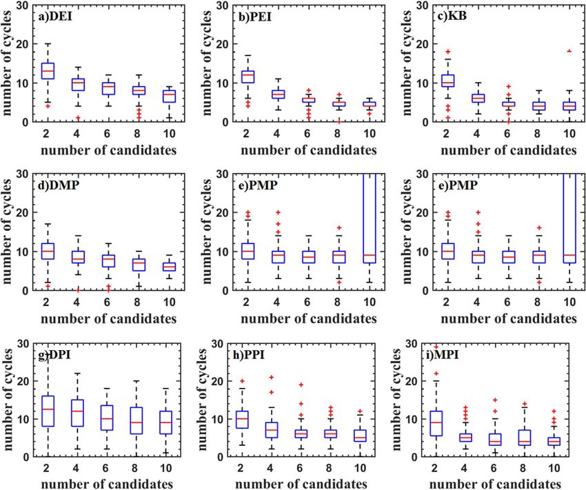
www.nature.com/scientificreports/
where κ is the improvement factor. The κ is set to 0.16.
The probability of improvement is described below:
T − ŷ(x)
PI(x) = � (10)
ŝ(x)
Pseudo expected improvement criterion. The principle is to reduce the value near the updated points
by introducing influence functions. The influence function is shown in (11)15.
IF x, x add = 1 − R x, x add (11)
The first updated point is identified by maximizing the standard EI function. As the optimization process
goes on, the q th updated point is identified as:
� � ��
x (n+q) = max PEI x, x (n+1) , . . . , x (n+q−1)
q−1 � � �� (12)
IF x, x ( )
�
n+q−1
= max EI(x) ∗
i=1
The detailed adding process can be seen at the end of this section. Similarly, we use the same steps to apply
the pseudo method to MP and PI criteria.
� � ��
x (n+q) = max PMP x, x (n+1) , . . . , x (n+q−1)
q−1 � � �� (13)
IF x, x ( )
�
n+q−1
= max MP(x) ∗
i=1
� � ��
x (n+q) = max PPI x, x (n+1) , . . . , x (n+q−1)
q−1 � � �� (14)
( )
�
n+q−1
= max PI(x) ∗ IF x, x
i=1
Distance function. Viana et al.17 introduced a fixed distance to constrain updated points. √ The distance of
each update point in each loop is greater than the given value. The distance is defined as 0.1 ∗ ndim . ndim is the
number of dimensions of the test problem. The parallel minimizing the prediction criterion with a fixed distance
to constrain is referred to as the MMP criterion. The parallel minimizing the prediction criterion with a fixed
distance to constrain updated points is referred to as the MMP criterion. The parallel probability of improve-
ment with a fixed distance to constrain updated points is referred to as the MPI criterion. The parallel expected
improvement with a fixed distance to constrain is referred to as the MEI criterion. The range of influence of the
real updated point is not the same as the given distance. So it is not reasonable to use a fixed distance directly. An
adaptive distance constraint is proposed based on the PEI. The method also uses correlation functions. When
the value of the correlation function is less than the threshold δ ∈ (0, 1), the value of the distance function is
1. Otherwise, it is 0. The distance function not only avoids the concentration of the candidate solution but also
improves the global searching ability. Because the hyper-parameters are anisotropic, so the distance function is
also anisotropic in all directions.
1 R
x, x add < δ
DIS x, x add = (15)
0 R x, x add > δ
Applying this method can refer to Viana’s17 or Zhan’s15. In this paper, the method of Zhan15 is taken as an
example. The qth updated point is identified as:
� � ��
x (n+q) = max DEI x, x (n+1) , . . . , x (n+q−1)
q−1 � � �� (16)
( )
�
n+q−1
= max EI(x) ∗ DIS x, x
i=1
Scientific Reports | (2022) 12:678 | https://doi.org/10.1038/s41598-021-04553-5 4
Vol:.(1234567890)
www.nature.com/scientificreports/
Figure 1. Flowchart of the parallel updated points.
� � ��
x (n+q) = max DMP x, x (n+1) , . . . , x (n+q−1)
q−1 � � �� (17)
( )
�
n+q−1
= max MP(x) ∗ DIS x, x
i=1
� � ��
x (n+q) = max DPI x, x (n+1) , . . . , x (n+q−1)
q−1 � � �� (18)
( )
�
n+q−1
= max PI(x) ∗ DIS x, x
i=1
Figure 1 shows the flowchart of the parallel updated points. The specific optimization process is as follows.
Step 1: Parameter initialization. The parameters, including design domain, boundary constraints, relative
parameters of the Kriging model, number of updating points, and convergence condition are initialized.
Step 2: Obtain initial samples by LHD.
Step 3: Build a Kriging model based on the current design samples.
Step 4: Take the expected improvement (EI) criterion as an example to illustrate the process of parallel add-
ing points.
(1) Pseudo method.
(a) Identify the first update point by looking for the maximum EI function value using GA.
(b) An approximation of the updated EI function is calculated by multiplying the initial EI function by
the influence function of the point x (n+1):
Scientific Reports | (2022) 12:678 | https://doi.org/10.1038/s41598-021-04553-5 5
Vol.:(0123456789)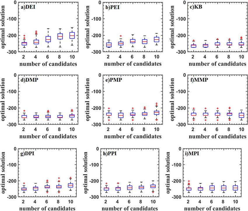
www.nature.com/scientificreports/
PEI x, x (n+1) = EI(x) ∗ IF x, x (n+1) (19)
(c) The second updating point is produced by maximizing the approximated updated EI function:
x (n+1) = max PEI x, x (n+1) (20)
(d) As the optimization process goes on, the q th updated point is identified as (13):
(2) Fix distance function method.
(a) Identify the first update point by looking for the maximum EI function value.
√
1 if Euclidean distance > 0.1 ∗ √ ndim
add
D x, x =
−1 else Euclidean distance > 0.1 ∗ ndim (21)
(b) The second updating point is identified as:
x (n+1) = max EI(x) ∗ D x, x (n+1) (22)
(c) As the optimization process goes on, the qth updated point is identified as:
x (n+q) = max EI(x) ∗ min D x, x (n+1) , D x, x (n+2) , . . . , D x, x (n+q) (23)
(3) Adaptive distance function.
(a) Identify the first update point by looking for the maximum EI function value.
(b) The second updating point is produced by maximizing the approximated updated EI function:
x (n+1) = max EI(x) ∗ DIS x, x (n+1) (24)
(c) As the optimization process goes on, the qth updated point is identified as (16):
Step 5: Convergence conditions. If the maximum number of function evaluations is met or the maximum
value of the EI is less than 0.1%, the whole loop is terminated. If it is not met, add the sampling points after the
choice to the sample set, and back to Step 3.
To make the progress of parallel adding points more intuitive, the author uses a one-dimensional function
in “Demonstrative example” to compare the process of single and parallel adding points.
Numerical experiments
Demonstrative example. The Forrester function19 y = (6x − 1)2 sin (12x − 4), x ∈ [0, 1] is used to
demonstrate the process of updating points. The initial sampling points are X = [0, 0.5, 0.7, 1]. Four updating
points are given in each cycle or iteration for the parallel criterion. Four cycles are demonstrated for the stand-
ard single-point criterion. Figure 2 shows the algorithm based on the EI criterion. The updated point position
of the PEI, DEI, and MEI criteria is close to the standard EI criterion. The difference is the order of adding the
point. For the KB criterion, the decay of the EI value is rapid because of the change of the hyper-parameter after
introducing the ‘fake’ point. The other three only construct the Kriging model once, so the EI function is real.
Therefore, it can be found that the parallel process essentially looks for other local optimal values. DEI and MEI
criteria are similar in the first cycle, but the distance function will change with the update of the Kriging model
for DEI. Figure 3 shows the algorithm based on the PI criterion. The updated points of the PI criterion are almost
consistent with the EI criterion, which shows that the PI criterion is also an effective infilling samples method.
And the updated points of MPI, PPI, and DPI criteria are also similar to the PEI, DEI, and MEI criteria. There-
fore, the parallel probability of improvement (PI) criterion can obtain effective updated points.
Figure 4 shows the algorithm based on the MP criterion. The standard MP criterion has the poor global
searching ability. Therefore, the candidate points are concentrated near the current optimal value. Although
the optimal solution can be found when the surrogate model is accurate, it is not conducive to improving the
prediction accuracy of the model. After the parallel criterion is introduced, the points near the candidate points
cannot be added so that the search expands outward. It is conducive to finding local optimal values and improv-
ing the global searching ability.
Through the demonstration of a one-dimensional function, the parallel criteria proposed in this paper can
effectively find update points after being introduced into the PI criterion. At the same time, the MP criterion can
be prevented from falling into the local optimum.
Test problems. Seven test problems are used for this experiment and described below.
Branin function with ndim = 2:
Scientific Reports | (2022) 12:678 | https://doi.org/10.1038/s41598-021-04553-5 6
Vol:.(1234567890)
www.nature.com/scientificreports/

                                 Figure 2.  KB, PEI, DEI, and MEI algorithm on Forrester function compared with the standard EI algorithm.

                                 Figure 3.  MPI, PPI and DPI algorithm on Forrester function compared with the standard EI algorithm.

                                                                            2
                                                                  5                         1
                                                f =       x2 −      x1 − 6        + 10 1 −      cos (x1 ) + 10, x1 ∈ [−5, 10], x2 ∈ [0, 15]     (25)
                                                                 4π                        8π
                                     Sasena function with ndim = 2:
                                                                        2
                                                   f = 2 + 0.01 x2 − x12 + (1 − x1 )2 2(2 − x1 ) + 7 sin (0.5x1 ) sin (0.7x1 x2 )

                                                                                                                                                (26)
                                                      x1,2 ∈ [0, 5]
                                     Hartman with ndim = 3 and ndim = 6:

Scientific Reports |   (2022) 12:678 |                https://doi.org/10.1038/s41598-021-04553-5                                                   7

                                                                                                                                              Vol.:(0123456789)
www.nature.com/scientificreports/
Figure 4. MMP, PMP, DMP algorithm on Forrester function compared with the standard EI.
4 n
� � � �2
f =− ci exp − αij xj − pij xi ∈ [0, 1], i = 1, 2, . . . , n
i=1 j=1
3 10 30
0.1 10 35
c = [1, 1.2, 3, 3.2], A(n = 3) = (27)
3 10 30
0.1 10 35
10 3 17 3.5 1.7 8
0.05 10 17 0.1 8.0 14
A(n = 3) =
3 3.5 1.7 10 17 8
17 8 0.05 10 0.1 14
0.3689 0.1170 0.2673
0.4699 0.4378 0.7470
P(n = 3) =
0.1091 0.8732 0.5547
0.03815 0.5743 0.8828
0.1312 0.1696 0.5569 0.0124 0.8283 0.5886
0.2329 0.4135 0.8307 0.3736 0.1004 0.9991
P(n = 3) =
0.2348 0.1451 0.3522 0.2883 0.3047 0.6650
0.4047 0.8828 0.8732 0.5743 0.1091 0.0381
StyblinskiTang7 with ndim = 7:
7
1
4
xi − 16xi2 + 5xi , xi ∈ [−5, 5], i = 1, 2, ..., 7 (28)
f =
2
i=1
Rosenbrock10 with ndim = 10:
9
2
100 xi+1 − xi2 + (xi − 1)2 , xi ∈ [−2, 2], i = 1, 2, ..., 10 (29)
f =−
i=1
Rastrigin12 with ndim = 12:
12
2
(30)
f = 120 + xi − 10 cos (2πxi ) , xi ∈ [−1, 3], i = 1, 2, ..., 12
i=1
Scientific Reports | (2022) 12:678 | https://doi.org/10.1038/s41598-021-04553-5 8
Vol:.(1234567890)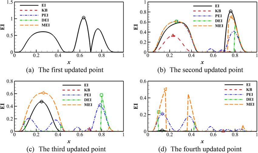
www.nature.com/scientificreports/
Figure 5. Test problems: Branin function.
Initial parameter setting. The initial sample uses the Latin hypercube design (LHD) function provided
by MATLAB. Kriging model is built using the DACE toolbox20. The infill sampling criterion is optimized by the
genetic algorithm provided by MATLAB. The settings are as follows.
• The number of initial points: 2 × (ndim + 1)
• Regression function: regpoly0.
• Correlation function: corrgauss.
• Initial hyperparameters:1
• Population size: 100
• Maximum iterations of GA: 100.
Test results. All parallel criteria are run to produce 2, 4, 6, 8, and 10 updated points in each cycle or iteration.
When the relative error of the optimal value is less than 0.01, we believe that convergence has been achieved. For
the first four test problems, the maximum number of cycles is 100. The number of cycles is counted when opti-
mization is done. The distance function threshold is set to 0.1. For the 5th to 7th test problems, because it is diffi-
cult to reach the optimal value for the high dimensional problems using 100 iterations. The maximum number of
cycles is set to 20, 40, 60, 80, corresponding to the process of adding 2, 4, 6, 8, and 10 update points. The optimal
value is counted, when the number of cycles reaches. The threshold value of the distance function is set to 0.5.
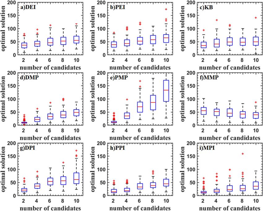
Figures 5, 6, and 7 show the boxplot of two and three-dimensional test problems. The median and interquartile
range of DEI, PEI, and KB criteria are close. The median and interquartile range of DEI is larger. The number
of cycles decreases with the updated point increasing. But the rate of decrease is slowing down, which indicates
that the optimization rate cannot increase linearly as the number of update points increases. KB criterion has
a lot of outliers when the updated point is great than two for the Branin function, which indicates that KB may
be invalid when the number of the parallel updated points added is large. For the two-dimensional test func-
tion, the PMP criterion converges faster when the updated points are two. As the number of updated points
increases, the number of iterations does not change much, indicating that the parallel infill sampling process
Scientific Reports | (2022) 12:678 | https://doi.org/10.1038/s41598-021-04553-5 9
Vol.:(0123456789)
www.nature.com/scientificreports/

                                           Figure 6.  Test problems: Sasena function.

                                           does not accelerate. The MMP criterion has the problem of falling into the local optima. DMP criterion improves
                                           this problem and is better than the result of using the EI parallel criterion. The optimization efficiency of the
                                           DMP criterion is increased by 20% compared with the PEI criterion in the two updating points process. As the
                                           number of points increases, the efficiency improvement is no longer obvious The law of the parallel method
                                           including the PI criterion is similar to that of the EI criterion. But the optimization converges speed is low. The
                                           convergence value is scattered and a large number of abnormal points appear. For the three-dimensional test
                                           function, the medians of PEI, PPI, KB, and MPI methods all have a significant improvement, and the distribu-
                                           tion of interquartile range is concentrated.
                                               Figure 8 shows the test result of the Hartman6 function. Although the median is low, the interquartile range
                                           of DEI, PEI, KB, PPI, DPI, and MMP criteria are scattered. The main reason is that these criteria always converge
                                           near the optimal value. It can also be seen from the inverse design of airfoil. The DMP and PMP criteria have a
                                           high median and a concentrated interquartile range indicating that these criteria are more robust.
                                               Figure 9 shows the test result of the StyblinskiTang7 function. With the increase of the number of updated
                                           points, the median of the optimal value is increased for DEI, PEI, DPI, MPI, PPI, and PMP criteria, which shows
                                           that the efficiency of parallel methods is reduced. The median of the optimal value of the KB, DMP, and MMP
                                           criteria is almost constant. The optimal values DMP criteria are low.
                                               The test result of the Rosenbrock10 function is shown in Fig. 10. When the updated points are two, DMP,
                                           PMP, DPI, MPI and PPI criteria have higher efficiency. As the updated points increase, the efficiency is gradually
                                           reduced. PMP criterion even traps in the local optimal solution. DEI, PEI, and KB criteria have a similar median.
                                           DMP, PPI, and MPI criteria have a smaller median.
                                               The test result of the Rastrigin12 function is shown in Fig. 11. It can be found that the optimal values obtained
                                           by DMP, PEI, and KB criteria are lower. And the interquartile range is narrower, but there are some outliers. The
                                           efficiency of parallel criteria for the high dimensional problems is decreased. KB criterion has a lower median
                                           and fewer outliers.

          Scientific Reports |   (2022) 12:678 |                https://doi.org/10.1038/s41598-021-04553-5                                                   10

Vol:.(1234567890)
www.nature.com/scientificreports/
Figure 7. Test problems: Hartman3 function.
The results of test functions show that the adaptive distance function proposed in this paper effectively
improves the problem that the traditional distance function is easy to fall into local optima. At the same time,
after it is introduced into the MP criterion, its optimization rate is also optimal.
After the pseudo method is introduced into the MP criterion, although the problem of falling into the local
optima is improved, the optimization rate is relatively slow. After the introduction of the PI criterion, the opti-
mization rate is similar. The optimization rate of the DEI method for low-dimensional problems is slower, but it
is not easy to fall into the local optima. The optimization rate of the DMP method is improved, and at the same
time, it does not fall into the local optima.
Application in the inverse design of airfoil
Demonstrative example. The efficient global optimization (EGO) algorithm based on the Kriging model
is widely used in airfoil design and optimization21,22. In this paper, the difference between the pressure distribu-
tion of the designed airfoil and the target pressure distribution is taken as the objective function. And the inverse
design problem is transformed into the optimization problem.
N
2
Obj. = Cpi − Ĉpi (21)
i=1
where the Cp is the pressure coefficient of the target airfoil and Ĉp is the pressure coefficient of the designed airfoil.
N is the number of points on the airfoil surface.
The inverse design of the airfoil is performed using the CST m ethod23–25. We first give a “thick” shape and
a “thin” shape and then fit the two shapes by CST. We consider the CST parameters of the “thin” shape as the
lower bound of the design variables and the parameters of the “thick” shape as the upper bound. The target
airfoil should be included in the design space. The design space is shown in Fig. 12. The fourth-order CST
method is used, and the total number of variables is 10. It can be seen from Fig. 13 that the RAE2822 airfoil can
be reproduced.
Scientific Reports | (2022) 12:678 | https://doi.org/10.1038/s41598-021-04553-5 11
Vol.:(0123456789)www.nature.com/scientificreports/
Figure 8. Test problems: Hartman6 function.
Numerical simulation method and verification. The two-dimensional mesh is generated by Gambit.
The computing domain shown in Fig. 14 is 70 m × 60 m, and the number of computing grids is about 220,000.
The numerical simulation is performed using ANSYS Fluent 14.0. The turbulence model is SST k–ω. The inlet
Mach number is 0.734, the inlet angle of attack is 2.79°. The Reynolds number is 6.5 × 10⁶. Figure 15 shows the
numerical results and the experimental results of the pressure distribution on the airfoil surface. The numerical
results are consistent with the experimental results. So the numerical method used in this paper has a high-level
accuracy.
The initial samples are generated by LHS, and the total number of samples is 40. First, three single point crite-
ria, EI, MP, and PI, are tested. The maximum number of cycles is set to 300. Later, parallel infill sampling criteria,
KB, PEI, DMP, PMP, and MPI, were tested. The maximum number of cycles is set to 300, 200, 100 corresponding
to adding 2, 3, and 6 updated points. A combination of the EI and MP method is also tested.
Figure 16 shows the result of the single updated point. The convergence curve of the MP criterion continues
to decrease. It converges to 0 after 120 cycles. The convergence rate of MP in the early stage is slower than the
others. The convergence rate of the PI is the fastest. EI and PI criteria only converge to about 0.3.
Figure 17 shows the result of two updated points. EI + MP, MPI, and DMP criteria have a higher convergence
rate. The convergence rate of the PMP criterion is gradually slowed down, but it can also converge to zero in the
end. The convergence rate and optimal value of the KB and PEI criteria are similar. The optimal value is about 0.3.
Figures 18 and 19 show the result of three and six updated points. KB has the fastest convergence rate, but
only converges to about 0.4. As the number of updated points increases, the convergence rate of PMP and DMP
criteria decreases. The optimal value still converges to 0. The convergence rate of PEI in the early stage decreases.
The overall efficiency increases.
The results of the inverse design of the airfoil show that the DMP criterion also shows a better convergence
rate and a smaller convergence value. The MPI method has a higher convergence rate in the early stage and the
Scientific Reports | (2022) 12:678 | https://doi.org/10.1038/s41598-021-04553-5 12
Vol:.(1234567890)www.nature.com/scientificreports/
Figure 9. Test problems: StyblinskiTang7 function.
optimal value is higher. Therefore, the MPI criterion can be used in the early stage to accelerate the convergence
speed in practical applications and later adopt the parallel method including MP criterion to obtain the optimal
value.
Conclusions
In this study, the “pseudo” method is applied to the MP criterion and PI criterion. An adaptive distance function
is proposed. Test problems were used to evaluate these criteria to verify the effectiveness of these methods. Some
parallel criteria are used in the inverse design of an airfoil to compare the differences between these methods in
the optimization speed and the optimal value, which can provide a reference for actual use selection.
After the pseudo method is introduced into the MP criterion, although the problem of falling into the local
optima is improved, the optimization rate is relatively slow. After the introduction of the PI criterion, the optimi-
zation rate is close to the PEI criterion. The optimization rate of the DEI method for low-dimensional problems
is slower, but it is not easy to fall into the local optima. The optimization rate of the DMP method is improved,
and at the same time, it does not fall into the local optima. Through the comparison of various parallel criteria,
the DMP, DMP, PPI, PEI, and KB methods have better convergence speed and robustness.
The results of the inverse design of airfoil show that the parallel methods including the MP criterion have the
best optimization value The convergence rate of the MPI is faster than the PEI and the KB, but the optimization
values are close. Moreover, the MPI criterion can be used in the early stage to accelerate the convergence speed
and later adopt the parallel method including the MP criterion to obtain the optimal value.
Scientific Reports | (2022) 12:678 | https://doi.org/10.1038/s41598-021-04553-5 13
Vol.:(0123456789)www.nature.com/scientificreports/
Figure 10. Test problems: Rosenbrock10 function.
Scientific Reports | (2022) 12:678 | https://doi.org/10.1038/s41598-021-04553-5 14
Vol:.(1234567890)www.nature.com/scientificreports/
Figure 11. Test problems: Rastrigin12 function.
Figure 12. The design space for RAE2822 airfoil.
Scientific Reports | (2022) 12:678 | https://doi.org/10.1038/s41598-021-04553-5 15
Vol.:(0123456789)www.nature.com/scientificreports/
0.1
0.08 RAE2822
CST
0.06
0.04
0.02
0
y
-0.02
-0.04
-0.06
-0.08
-0.1
0 0.2 0.4 0.6 0.8 1
x
Figure 13. Comparison of the shapes of the designed airfoil and target airfoil.
Figure 14. Sketch of mesh for numerical calculation.
1.5
CFD
1 EXP
0.5
0
Cp
-0.5
-1
-1.5
0 0.2 0.4 0.6 0.8 1
x/C
Figure 15. Comparison of CFD and experimental data.
Scientific Reports | (2022) 12:678 | https://doi.org/10.1038/s41598-021-04553-5 16
Vol:.(1234567890)www.nature.com/scientificreports/
Figure 16. Convergence history of single updated point.
Figure 17. Convergence history of two updated points.
Figure 18. Convergence history of three updated points.
Scientific Reports | (2022) 12:678 | https://doi.org/10.1038/s41598-021-04553-5 17
Vol.:(0123456789)www.nature.com/scientificreports/
Figure 19. Convergence history of six updated points.
Data availability
The authors declare that the data supporting the findings of this study are available within the paper and addi-
tional data on methods used are available upon reasonable request.
Received: 12 August 2021; Accepted: 20 December 2021
References
1. Cheng, S. X., Zhan, H., Shu, Z. X., Fan, H. Y. & Wang, B. Effective optimization on Bump inlet using meta-model multi-objective
particle swarm assisted by expected hyper-volume improvement. Aerosp. Sci. Technol. 87, 431–447. https://doi.org/10.1016/j.ast.
2019.02.039 (2019).
2. Kuhnt, S. & Steinberg, D. M. Design and analysis of computer experiments. Asta Adv. Stat. Anal. 4, 409–423 (1989).
3. Han, Z. H., Gortz, S. & Zimmermann, R. Improving variable-fidelity surrogate modeling via gradient-enhanced Kriging and a
generalized hybrid bridge function. Aerosp. Sci. Technol. 25, 177–189. https://doi.org/10.1016/j.ast.2012.01.006 (2013).
4. Bhattrai, S., de Baar, J. H. S. & Neely, A. J. Efficient uncertainty quantification for a hypersonic trailing-edge flap, using gradient-
enhanced kriging. Aerosp. Sci. Technol. 80, 261–268. https://doi.org/10.1016/j.ast.2018.06.036 (2018).
5. Jones, D. R., Schonlau, M. & Welch, W. J. Efficient global optimization of expensive black-box functions. J. Glob. Optim. 13, 455–492.
https://doi.org/10.1023/A:1008306431147 (1998).
6. Liu, J., Song, W. P., Han, Z. H. & Zhang, Y. Efficient aerodynamic shape optimization of transonic wings using a parallel infilling
strategy and surrogate models. Struct. Multidiscip. Optim. 55, 925–943. https://doi.org/10.1007/s00158-016-1546-7 (2017).
7. Forrester, A. I. J. & Keane, A. J. Recent advances in surrogate-based optimization. Prog. Aerosp. Sci. 45, 50–79. https://doi.org/10.
1016/j.paerosci.2008.11.001 (2009).
8. Ginsbourger, D., Le Riche, R. & Carraro, L. Kriging is Well-Suited to Parallelize Optimization 131–162 (Springer, 2010).
9. Sobester, A., Leary, S. J. & Keane, A. J. A parallel updating scheme for approximating and optimizing high fidelity computer simula-
tions. Struct. Multidiscip. Optim. 27, 371–383. https://doi.org/10.1007/s00158-004-0397-9 (2004).
10. Feng, Z. W. et al. A multiobjective optimization based framework to balance the global exploration and local exploitation in
expensive optimization. J. Glob. Optim. 61, 677–694. https://doi.org/10.1007/s10898-014-0210-2 (2015).
11. Li, C., Guo, Z. & Song, L. Design Optimization of a 3D Parameterized Vane Cascade With Non-Axisymmetric Endwall Based on
a Modified EGO Algorithm and Data Mining Techniques. In ASME GT2017-63738 (2017).
12. Li, Y., Shen, J. & Cai, Z. A Kriging-assisted multi-objective constrained global optimization method for expensive black-box func-
tions. Mathematics. 9(2), 149 (2021).
13. Li, Y., Wang, S. & Wu, Y. Kriging-based unconstrained global optimization through multi-point sampling. Eng. Optim. 52, 1082–
1095 (2020).
14. Viana, F. A. C., Haftka, R. T. & Watson, L. T. Efficient global optimization algorithm assisted by multiple surrogate techniques. J.
Glob. Optim. 56, 669–689. https://doi.org/10.1007/s10898-012-9892-5 (2013).
15. Zhan, D. W., Qian, J. C. & Cheng, Y. S. Pseudo expected improvement criterion for parallel EGO algorithm. J. Glob. Optim. 68,
641–662. https://doi.org/10.1007/s10898-016-0484-7 (2017).
16. Song, C., Yang, X. D. & Song, W. P. Multi-infill strategy for Kriging models used in variable fidelity optimization. Chinese J. Aero-
naut. 31, 448–456. https://doi.org/10.1016/j.cja.2018.01.011 (2018).
17. Viana, F. A. Multiple Surrogates for Prediction and Optimization (University of Florida, 2011).
18. Li, Y. H. A Kriging-based global optimization method using multi-points infill search criterion. J. Algorithms Comput. 11, 366–377.
https://doi.org/10.1177/1748301817725307 (2017).
19. Forrester, A. I. J., Sobester, A. & Keane, A. J. Engineering Design Via Surrogate Modelling: A Practical Guide (Wiley, 2008).
20. Lophaven, S. N., Nielsen, H. B. & Søndergaard, J. DACE: A Matlab Kriging Toolbox (The Technical University of Denmark, 2002).
21. Bartoli, N., Lefebvre, T. & Dubreuil, S. Adaptive modeling strategy for constrained global optimization with application to aero-
dynamic wing design. Aerosp. Sci. Technol. 90, 85–102 (2016).
22. Alba, C., Elham, A., German, B. J. & Veldhuis, L. L. L. M. A surrogate-based multi-disciplinary design optimization framework
modeling wing-propeller interaction. Aerosp. Sci. Technol. 78, 721–733. https://doi.org/10.1016/j.ast.2018.05.002 (2018).
23. Kulfan, B. M. Recent extensions and applications of the “CST” universal parametric geometry representation method. Aeronaut.
J. 114, 157–176. https://doi.org/10.1017/S0001924000003614 (2010).
24. Kulfan, B. M. Universal parametric geometry representation method. J. Aircraft. 45, 142–158. https://doi.org/10.2514/1.29958
(2008).
Scientific Reports | (2022) 12:678 | https://doi.org/10.1038/s41598-021-04553-5 18
Vol:.(1234567890)www.nature.com/scientificreports/
25. Du, X. S., Ren, J. & Leifsson, L. Aerodynamic inverse design using multifidelity models and manifold mapping. Aerosp. Sci. Technol.
85, 371–385. https://doi.org/10.1016/j.ast.2018.12.008 (2019).
Author contributions
C.C. gives the main idea of work. This author was responsible for collecting and analyzing data and writing drafts
of the manuscript. L.J.: responsible for editing significant drafts of the manuscript. X.P.: responsible for assisting
with super-computing, providing software, revising drafts of the manuscript and CFD analyses.
Competing interests
The authors declare no competing interests.
Additional information
Correspondence and requests for materials should be addressed to C.C.
Reprints and permissions information is available at www.nature.com/reprints.
Publisher’s note Springer Nature remains neutral with regard to jurisdictional claims in published maps and
institutional affiliations.
Open Access This article is licensed under a Creative Commons Attribution 4.0 International
License, which permits use, sharing, adaptation, distribution and reproduction in any medium or
format, as long as you give appropriate credit to the original author(s) and the source, provide a link to the
Creative Commons licence, and indicate if changes were made. The images or other third party material in this
article are included in the article’s Creative Commons licence, unless indicated otherwise in a credit line to the
material. If material is not included in the article’s Creative Commons licence and your intended use is not
permitted by statutory regulation or exceeds the permitted use, you will need to obtain permission directly from
the copyright holder. To view a copy of this licence, visit http://creativecommons.org/licenses/by/4.0/.
© The Author(s) 2022
Scientific Reports | (2022) 12:678 | https://doi.org/10.1038/s41598-021-04553-5 19
Vol.:(0123456789)You can also read