Graphics with MAXIMA (Version 5.23 and above) - Wilhelm Haager HTL St. Pölten, Department Electrical Engineering
←
→
Page content transcription
If your browser does not render page correctly, please read the page content below
Graphics with MAXIMA
            (Version 5.23 and above)

                 Wilhelm Haager
HTL St. Pölten, Department Electrical Engineering
          wilhelm.haager@htlstp.ac.at

                November 26, 2011
Contents ii Contents 1 Basics 1 2 Gnuplot 3 2.1 Gnuplot Commands . . . . . . . . . . . . . . . . . . . . . . . . . . . . . . . . . . . . . . . 3 2.2 Gnuplot Terminals . . . . . . . . . . . . . . . . . . . . . . . . . . . . . . . . . . . . . . . . 4 2.3 Initialization . . . . . . . . . . . . . . . . . . . . . . . . . . . . . . . . . . . . . . . . . . . . 5 3 Graphic Interface Plot 6 3.1 Plot Commands . . . . . . . . . . . . . . . . . . . . . . . . . . . . . . . . . . . . . . . . . . 6 3.2 Options . . . . . . . . . . . . . . . . . . . . . . . . . . . . . . . . . . . . . . . . . . . . . . . 10 4 Graphic Interface Draw 14 4.1 Plot Commands . . . . . . . . . . . . . . . . . . . . . . . . . . . . . . . . . . . . . . . . . . 14 4.2 2d-Graphic Objects . . . . . . . . . . . . . . . . . . . . . . . . . . . . . . . . . . . . . . . . 15 4.3 3d-graphic objects . . . . . . . . . . . . . . . . . . . . . . . . . . . . . . . . . . . . . . . . 19 4.4 General Options . . . . . . . . . . . . . . . . . . . . . . . . . . . . . . . . . . . . . . . . . 22 4.5 Options for Labels and Vectors . . . . . . . . . . . . . . . . . . . . . . . . . . . . . . . . 26 4.6 Options for 2d-Graphics . . . . . . . . . . . . . . . . . . . . . . . . . . . . . . . . . . . . . 27 4.7 Options for 3d-Graphics . . . . . . . . . . . . . . . . . . . . . . . . . . . . . . . . . . . . . 29 Bibliography 32
1 Basics 1
1 Basics
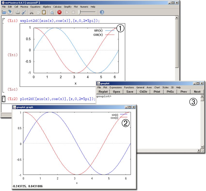
Maxima uses the program Gnuplot for depicting graphics [2], which is called automatically,
when the graphic is produced. Two various methods for displaying the graphics are possible:
1. When calling the standard plotting routines plot2d, plot3d, draw2d, draw3d, etc., a Gnu-
plot output window containing the graphic is popping up. Continuing working with Max-
ima is not possible until that window is closed again. The Gnuplot output window and
➀ . . . Graphic in wxMaxima working window
➁ . . . Graphic in Gnuplot output window
➂ . . . Gnuplot console
Wilhelm Haager: Graphics with MAXIMA1 Basics 2
consequently the graphic too can be resized using the mouse. Measurements can be per-
formed in 2d-plots with the mouse, 3d-plots can be rotated in any arbitrary direction.
Right-clicking the window title opens a context menu, which enables printing the graphic
and opening the Gnuplot console. Using that console window, Gnuplot can be used as a
separate program, even independently of Maxima.
2. When preceeding the letters “wx” to the names of the plotting routines (wxplot2d,
wxplot3d, wxdraw2d, wxdraw3d, . . . ), PNG-graphics are produced in screen resolution and
placed directly into the wxMaxima working window. As the graphics remain visible during
the entire Maxima session, that method is beneficial for interactive work. Right clicking
the graphic enables copying into the clipboard or saving as a file. Nevertheless, due to its
low resolution, further use of a graphic produced in that way is not reasonable.
Two various Gnuplot interfaces are available, the Maxima standard functions with the stem
“plot” in the function names, as well as the routines of the additional package Draw [3] with the
stem “draw” in the function names.
The routines of the package Draw are admittedly slightly more complicated concerning their
usage, but they are more flexible than the standard routines and offer much more possibilities
to adapt the graphics with the aid of options to particular requirements. Furthermore it is
possible, to set output format (eps, png, jpg, etc.) and output target (i. e. the filename) in the
gnuplot console after the graphic has been produced, which is appearently not possible when
using the standard routines of the Gnuplot interface Plot.
Wilhelm Haager: Graphics with MAXIMA2 Gnuplot 3
2 Gnuplot
Gnuplot is a comand-line oriented plot program. When called by Maxima, the input of com-
mands into the Gnuplot console window is not necessary in general, but can be helpful, espe-
cially when using the Gnuplot interface Draw. For that reason the basic principles and the (few)
most inportant commands of Gnuplot are explained below.
2.1 Gnuplot Commands
plotf(x) opts Plotting the function f(x) with the options opts;
fundamental command for producing graphics, but
there is no need for it within Maxima.
replot Plotting a graphic anew, occasionally with changed
settings
set terminal term opts Setting the output format, if necessary, with additional
options opts.
set output "filename" Setting the output target (filename with the
appropriate extension)
set size xscale,yscale Scaling the diagram with respect to the size of the
entire grafic
set size ratio n Sets the aspect ratio height/width of the diagram
show item Shows the actual value of item.
cd "directory" Changes the working directory for the output file
pwd Shows the working directory
load "filename" Loads a batch of Gnuplot commands from the file
filename.
set/unset key Turns the lege!ison/off
set/unset hidden3d Turns the visibility of hidden lines in 3d-plots on/off
set/unset grid Turns the coordinate grid on /off
set cntrparam spez Controls contour lines in a contour-plot
set view rotx rotz scale scaley Sets the view point of 3d-plots
quit Exiting Gnuplot; not used within Maxima.
Important Gnuplot Commands
Gnuplot commands are input into the Gnuplot console line by line; one line can contain sev-
eral commands, separated by semicolons. Commands and parameters are separated by spaces,
particular coordinates by colons. Coordinate ranges have the form [ x 1 : x 2 ].
Wilhelm Haager: Graphics with MAXIMA2 Gnuplot 4
The basic plot command plot is called by Maxima automatically, when a diagram is produced;
input of that command by the user does not make sense.
When using the Gnuplot interface Draw, an existing graphic can be drawn anew using the
command replot, if necessary with changed settings, assigned with the command set and
shown with the command show.
set terminal (abbreviated set term) assigns the file format of the produced graphic. A plethora
of formats is available [2], the most important ones are shown in section 2.2 below.
set output assigns the output target, i. e. the name of the graphic file. Unless the entire file
path is given as the parameter, but only the filename, the file is saved in the current working
directory (assigned with cd, shown with pwd). The file name stdout causes the graphic to be
drawn into the Gnuplot output window, regardless of the Gnuplot terminal assigned.
The command set output should always be performed after the eventual command set terminal.
The command set size does not assign the size of the entire graphic, but the size of the diagram
within the graphic with respect to its standard size. Values greater than 1 cause clipping parts of
the diagram. set size ratio assigns the aspect ratio height/width of the diagram, a negative
value does not set the ratio of the lengths of the axes, but the ratio of their scales. Thus for
example set size ratio -1 causes the same scale of the x- and y-axis (and not the same
lengths); in that case e. g. a circle remains an undistorted cirle.
The command set cntrparam sets the number and values of the contour lines in contour-plots
in various ways:
set cntrparam levels n . . . automatic calculation of n contour lines
set cntrparam discrete z1,z2,. . . . . . assigning particular values for contour lines
set cntrparam incremental z1,dz,z2 . . . contour lines ranging from z1 to z2 with an
interval of dz
set view rotx rotz scale scalez sets the view of 3d-plots. Herein rotx is the rotation around the
x-axis (starting from vertical view), rotz the rotation around the z-axis scale a global scale factor
and scalez an additional scale factor of the z-axis.
The command load starts batch processing of Gnuplot commands, which are stored in a textfile.
2.2 Gnuplot Terminals
Most Gnuplot terminals offer additional options, which allow adapting the graphic with respect
to resolution, size, color depth, font and font size. Unfortunaely the number and the format of
those options are not coherent for all terminals, in particular the Gnuplot manual or [2] has to
be consulted.
Wilhelm Haager: Graphics with MAXIMA2 Gnuplot 5
Pixel Formats:
dumb retro-style ASCII-art graphic
gif GIF-graphic (suitable for web pages), 8 bit color depth
png Portable Network Graphics, developed in order to
replace GIF, 24 bit color depth
jpeg JPG-graphic
latex LATEX-code with the picture environment
windows on-screen display in the Gnuplot output window
Vector Formats:
aifm Adobe-Illustrator format (file extension .ai)
dxf AutoCAD drawing interchange format
eepic LATEXcode with the extended picture environment
(requires the package eepic)
hpgl Hewlett-Packard Graphics Language for pen-plotters
and CNC milling machines
postscript Postscript graphic (file extension .ps)
postscript eps Encapsulated Postscript graphic (file extension .eps)
svg Scalable Vector Graphics
Important Gnuplot terminals
2.3 Initialization
gnuplot.ini initialization file for graphic settings
wgnuplot.ini initialization file for Gnuplot settings (i. e. the visual
appearance of Gnuplot)
GNUPLOT environment variable, contains the path name of the
initialization files.
Gnuplot-Initialization
Favored standard settings for producing graphics, e. g. the Gnuplot working directory, can be
assigned in a file named gnuplot.ini. That file can contain any Gnuplot commands, which are
performed at starting Gnuplot.
Standard settings for the appearance of Gnuplot itself, e. g. text size and window size of the
gnuplot console, are assigned in the file wgnuplot.ini. That File is not created by the user
directly, but via the context menu of of the Gnuplot console.
The directories containing the initialization files gnuplot.ini and wgnuplot.ini are assigned
in the environment variable GNUPLOT.
Wilhelm Haager: Graphics with MAXIMA3 Graphic Interface Plot 6
3 Graphic Interface Plot
Plot is the standard Gnuplot interface of Maxima, convenient in its application, but not very
flexible regarding the graphics’ appearance. Furthermore, the possibilities for producing 3d-
graphics are very limited. When using this interface, it is unfortunately not possible, to change
appearance, output format or output target of a graphic in the Gnuplot console after the graphic
has been drawn.
3.1 Plot Commands
plot2d(f(x),xrange,opts) Plots the function f(x) with the options opts within the
range xrange; xrange must be declared.
plot2d([discrete,xwerte,ywerte],opts)
Plots the points with declaration of x-values and
y-values in two distinct lists xwerte and ywerte; the
declaration of a range for the x-values is optional.
plot2d([discrete,werte],opts)
Other possibility for plotting points; the points are
given in a nested list [[x1,y1],[x2,y2],...].
plot2d([parametric,x(t),y(t),trange],opts)
Plots a parametric curve with the parameter t within
the range trange
plot3d(f(x,y),xrange,yrange,opts)
Plots a function f(x,y) with the options opts within the
rangs xrange and yrange
plot3d([x(u,v),y(u,v),z(u,v)],urange,vrange,opts)
Plots a parametric surface with the parameters u and v
within the ranges urange and vrange
contour_plot(f(x,y),xrange,yrange,opts)
Plots contour lines of a function f(x,y) with the options
opts within the ranges xrange and yrange
[x,x1,x2] Declaration of a range for the variable x with the lower
bound x1 and the upper bound x2
Plot commands of the Gnuplot interface Plot
The command (wx)plot2d draws a curve or line segments between a couple of points in a two-
dimensional cartesian coordinate system. There are three possibilities for that, which can be
combined arbitrarily in one single diagram:
Wilhelm Haager: Graphics with MAXIMA3 Graphic Interface Plot 7
1. A function y = f (x); the displayed range along the x-axis must be declared as [x,x1,x2],
declaration of y-range is optional.
2. A curve in parametric form x(t), y(t) in dependence of an arbitrarily choosable parameter
t . If that parameter has actually the name „t“, the declaration of a range can be omitted.
In that case t gets the default values as declared with set_plot_option. (the same value
for all parametric curves) (section 3.2).
3. Particular points, which can be connected (applying the respective options) by line seg-
ments. There are two possibilities for the specification of the points: either in two par-
ticular lists containing the x-values and the y-values respectively, or in a single nested list
containing the points, each point representing a list containing its x-value and y-value.
Plotting a function within a declared (%i1) wxplot2d(sin(x),[x,-%pi,%pi])$
range; the range of the y-axis is
calculated automatically.
(%t1)
Declaration of x-values in a list: (%i2) xwerte:[0,3,6,4,6,3,0,2,0];
(%o2) [0, 3, 6, 4, 6, 3, 0, 2, 0]
Declaration of y-values in a list: (%i3) ywerte:[0,2,0,3,6,4,6,3,0];
(%o3) [0, 2, 0, 3, 6, 4, 6, 3, 0]
Two pointwise plots in one diagram with (%i4) wxplot2d([[discrete,xwerte,ywerte],
both ways declaring the points. The [discrete,[[3,1],[5,3],[3,5],[1,3],[3,1]]]])$
points are connected by line segments by
default.
(%t4)
Wilhelm Haager: Graphics with MAXIMA3 Graphic Interface Plot 8
Curve in paramettic form; in order to (%i5) wxplot2d([parametric,sin(t),sin(2*t),
achieve a smooth curve, the number of [t,0,2*%pi]],[nticks,100])$
initial points has to be increased using
the option nticks.
(%t5)
Combination of three vatious 2d-plots in (%i6) wxplot2d([sin(x),[discrete,xwerte,ywerte],
one single diagram; the three respective [parametric,10+3*sin(2*t),2+2*cos(3*t),
expressions have to be put into a list. [t,0,2*%pi]]],[x,0,15],[nticks,100])$
(%t6)
One single diagramm can contain any number of curves, put together in a list.
The Gnuplot interface Plot offers only very limited possibilities for creating 3d-plots, they are
described below only for the sake of completeness. Anyway, the use of the Gnuplot interface
Draw is recommended for the creation of 3d-graphics.
Two kinds of 3d-objects can be produced; however, only one single object can be drawn into a
3d-graphic:
1. A function z = f (x, y); the ranges for x-values and y-values have to be declared. However,
the z-range cannot be declared.
2. An object in parametric form x(u, v), y(u, v), z(u, v) in dependence of two (arbitrarily chooseable)
parameters u and v . The ranges of the parameters u and v have to be declared, the ranges
of the coordinates x , y and z cannot be declared.
Wilhelm Haager: Graphics with MAXIMA3 Graphic Interface Plot 9
3d-plot of a function in two variables; (%i7) wxplot3d(1/(1+x^2+y^2),[x,-3,3],[y,-3,3])$
declaration of the ranges for x and y are
optional, their default values are stored
in the list plot_options.
(%t7)
Parametric form of a surface in (%i8) [fx:cos(x),fy:y,fz:sin(x)+y^2];
three-dimensional space
(%o8) [cos (x) , y, y 2 + sin (x)]
3d-plot of a surface in parametric form (%i9) wxplot3d([fx,fy,fz],[x,0,2*%pi],[y,0,1],
[palette,false])$
(%t9)
contour_plot draws contour lines of a function in two variables within the ranges xrange
and yrange, the number and the values of the contour lines can be declared using the option
gnuplot_preamble (sections 2.1 und 3.2).
Contour lines of a function in two (%i10) wxcontour_plot(1/(1+x^2+y^2),
variables. An explicit declaration of the [x,-3,3],[y,-3,3])$
function values for the lines, as well as
turning off the legend, using the
appropriate options, would be benefical.
(%t10)
Wilhelm Haager: Graphics with MAXIMA3 Graphic Interface Plot 10
3.2 Options
Additional optional parameters allow adapting a graphic to particular requirements with respect
to colors, line types, sizes, labels, output formats etc. The options are lists (mostly containing
two elements); the first element is always the name of the option, additional elements are the
associated values.
Options can be stated as additional parameters in every plot command; they can also be de-
clared as default values using the command set_plot_option. In that case they are valid for
all subsequent plot commands. The command plot_options shows all default values of the
options.
Commands:
plot_options Shows all options
set_plot_option([name,v]) Assigns the option name to the value v
Important options:
[y, ymin, ymax] Range of the y-axis
[x, xmin, xmax] Range of the x-axis, obligatory in 2d-plots, optional in
3d-plots
[nticks,n] Number of initial points for calculation of a curve
(default:10)
[adapt_depth, n] Maximum number of curve secions between two initial
points (Default:10)
[gnuplot_preamble, "text"] Gnuplot preamble, contains Gnuplot commands, which
precede the plot.
[xlabel,"text"] x-axis label in 2d-plots
[ylabel,"text"] y-axis label in 2d-plots
[logx]/[logy] Logarithmic scaling of the x-/y-axis in 2d-Plots
[legend,"text1","text2",...] Legends for particular curves in a 2d-Plot
[style,style1,style2,...] plot styles for the particular curves in a 2d-plot in the
form [name,w,c]
[gnuplot_term, terminal] Output format (i. e. the Gnuplot terminal); ignored by
the wx-routines
[gnuplot_out_file, "filename"]
Output target; ignored by the wx-routines
[grid,nx,ny] Number of grid lines in 3d-plots in x- and y-direction
respectively
[gnuplot_pm3d, true/false] Controls coloring of surfaces in 3d-plots
Plot options for the Gnuplot interface Plot
Wilhelm Haager: Graphics with MAXIMA3 Graphic Interface Plot 11
The options x and y declare the displayed coordinate ranges, in 2d-plots x is obligatory.
nticks and adapt_depth set the number and maximum division of initial points for calculat-
ing the curve. If the displayed curves are sufficiently “smooth”, its explicit declaration is not
necessary.
The option gnuplot_preamble can contain any number of Gnuplot commands as a text string,
the particular Gnuplot commands are separated by semicolons. They are carried out prior the
actual plotting process. Hence settings can be passed to Gnuplot, which cannot be controlled by
Maxima’s plot options. (e. g. controlling the contour lines in contour plots or setting the aspect
datio of diagrams).
Lissajous curve; the option (%i11) wxplot2d([parametric,sin(3*t),sin(4*t),
gnuplot_preamble enforces equal scales [t,0,2*%pi]],[nticks,100],
for both axes, the option nticks [gnuplot_preamble,"set size ratio -1"])$
increases the number of calculated
points in order to get a smooth curve.
(%t11)
The option style assigns the type of the curve, line width and line color (and the point type, if
desired). In pixel graphics the line width is given in pixels, in vector graphics as multiples od
0.25pt (about 0.088mm). The curve type can obtain the following values:
lines . . . solid line
points . . . points (with an additional integer number assigning the point type)
linespoints . . . solid line and points
impulses . . . bars (line widths and colors are ignored)
Colors can have the following values:
1 . . . blue 2 . . . red
3 . . . magenta 4 . . . yellow
5 . . . brown 6 . . . green
7 . . . cyan
List containing x-values (%i12) lx:[1,2,3,4,5,6,7,8,9];
(%o12) [1, 2, 3, 4, 5, 6, 7, 8, 9]
List containing y-values (%i13) ly:[1,2,2.4,2.4,1.7,1.5,1.6,2,2.7];
(%o13) [1, 2, 2.4, 2.4, 1.7, 1.5, 1.6, 2, 2.7]
Wilhelm Haager: Graphics with MAXIMA3 Graphic Interface Plot 12
Plotting points in various plot styles: as (%i14) wxplot2d(makelist([discrete,lx,c+ly],c,1,4),
line segments, as points (in various sizes [x,0,10],[y,1,8],[legend,""],
and shapes) and as a combination of [style,[lines,2,1],[points,2,6,1],
both. [points,4,2,7],[linespoints,3,4,3]])$
(%t14)
(Somewhat tricky) generation of a list of (%i15) plotlist:apply(append,makelist(makelist
point plots containing one single point ([discrete,[[nx,ny]]],nx,1,13),ny,1,7))$
each
(Somewhat tricky) generation of a list of (%i16) stylelist:cons(style,apply(append,makelist(
plot styles in all colors and all point makelist([points,4,ny,nx],nx,1,13),ny,1,7)))$
types
Plotting all possible colors and point (%i17) wxplot2d(plotlist,stylelist,[x,0,14],[y,0,8],
types. Appropriate options suppress the [legend,""],[xlabel,"Point numbers"],
legend and assign labels for the axes. [ylabel,"Color numbers"])$
(%t17)
gnuplot_term assigns the output format; beside the values default and ps (for encapsulated
postscript) all Gnuplot terminals (section 2.2) are possible. The option gnuplot_out_file as-
signs the output target file. Unless the entire file path is given, (inexplicably) not the Gnuplot
working directory will be used, but the user home directory as declared in the environment
variable HOMEPATH. gnuplot_term and gnuplot_out_file are ignored by the wx-routines.
3d-Plots provide only bare possibilities for changing the settings. The option gnuplot_preamble
allows assigning settings directly in Gnuplot:
Generation of a Gnuplot preamble for (%i18) p:"unset hidden3d;set view 20,10,1,3";
3d-plots in order to show hidden lines
(%o18) unset hidden3d;set view 20,10,1,3
and change the view point
Wilhelm Haager: Graphics with MAXIMA3 Graphic Interface Plot 13
3d-plot with a Gnuplot preamble, (%i19) wxplot3d(1/(1+x^2+y^2),[x,-3,3],[y,-3,3],
changes number of grid lines and [grid,60,60],[gnuplot_preamble, p],
turned-off color palette [palette,false])$
(%t19)
Wilhelm Haager: Graphics with MAXIMA4 Graphic Interface Draw 14
4 Graphic Interface Draw
The Gnuplot interface Draw by Mario Rodríguez Riotorto [3] provides an additional set of Max-
ima graphic routines, which differ from the standard routines with regard to their parameters,
in particular the structure of the options.
The application of these routines, all having the stem “draw” in their function names, is slightly
more complicated than of the standard routines. However, they offer much more flexibility for
configuration and adapting the graphics to particular requirements. Moreover, output format
and output target can be assigned after the graphic has been drawn into the Gnuplot output
window.
The package Draw has to be loaded prior to its first use.
4.1 Plot Commands
draw(scene1,scene2,...,opts,...)
Creation of a graphic as a compilation of Szenen and
global options opts.
gr2d(opts,graphic_object,...) Creation of a 2d-scene as a compilation of arbitrary 2d
graphic objects with the options opts
gr3d(opts,graphic_object,...) Creation of a 3d-scene as a compilation of arbitrary 3d
graphic objects with the options opts
draw2d(opts,graphic_object,...)
Creation of a 2d-graphic as a compilation of arbitrary
2d graphic objects with the options opts
draw3d(opts,graphic_object,...)
Creation of a 2d-graphic as a compilation of arbitrary
2d graphic objects with the options opts
Options:
name1=value1,name2=value2,...
Plot commands of the Gnuplot interface Draw
A graphic consists of particular (2d- and 3d-) scenes, which are output by the basic plot command
draw in a rectangle array, each scene containing a single diagram.
A scene, a compilation of several graphc objects and (if desired) additional options, is created
with the commands gr2d (for 2d-graphics) and gr3d (for 3d-graphics).
Wilhelm Haager: Graphics with MAXIMA4 Graphic Interface Draw 15
Most graphic contain only one single diagram (i. e. only one single scene). In that case the plot
commands draw2d and draw3d compile the graphic objects to a scene and draw the graphic for
that scene in one single step. Thus The commands
draw2d(...) and draw3d(...)
are equal to
draw(gr2d(...)) and draw(gr3d(...)).
The parameter list contains any number of graphic objects and options. Options referring to a
particular graphic object must precede that object. The position of global parameters (e. g. for
declaring output format and output target) is arbitrary.
Options are declared as equations with its name on the left hand side and its value on the right
hand side. The value can also be a list (e. g. for assigning ranges with lower bound and upper
bound).
At complex graphics containing many objects, the parameter list can get long and somewhat
confusing. In that case it is good style, either
• to structure the input by appropriate line breaks and indentations, or (even better)
• not to declare the graphic objects directly in the parameter list of the plot commands, but
assign variable names to them in separate commands and use those variable names in the
parameter list of the plot commands.
4.2 2d-Graphic Objects
explicit, parametric and implicit create graphic objects from mathematical expressions in
cartesian coordinates. polar creates a graphic object of a function in polar coordinates. As the
displayed ranges are an inherent part of the graphic objets, they need not be declared—contrary
to the Gnuplot interface Plot—as options.
Furthermore, a number of geometric shapes is available, which allow the composition of ar-
bitrary graphics. The graphic object points primarily displays a number of discrete points.
Applying the approptiate options, those points can be connected by line segments. Thus points
enables the creation of any graphic consisting of lines and approximate curves (section 4.4).
Wilhelm Haager: Graphics with MAXIMA4 Graphic Interface Draw 16
explicit(f(x),x,x1,x2) Function f(x) within the range of x1 and x2
parametric(x(t),y(t),t,t1,t2)
Parametric curve x(t),y(t) with the parameter t ranging
from t1 to t2
implicit(equation,x,x1,x2,y,y1,y2)
Implicit curve, declared by the equation equation, with
the variables x and y within the ranges x1. . . x2 and
y1. . . y2
polar(r(ϕ ),ϕ ,ϕ 1,ϕ 2) Function in polar coordinates; radius r with respect to
the angle ϕ in degree ranging from ϕ 1 to ϕ 2
points(xvals,yvals) Points; xvals and yvals are lists containing the x- and
y-values respectively
points(p1,p2,...) Points; each ponint pi is a list with its coordinates:
[px,py].
polygon(xvals,yvals) Polygon with declaration of its vertexes in lists xvals
and yvals.
polygon(p1,p2,...) Polygon; each vertex pi is a list containing its
coordinates: [px,py].
rectangle(p1,p2) Rectangle with the opposite vertexes p1 and p2 in the
form [px,py]
ellipse(x0,y0,a,b,w1,w2) Ellipse (oder circle) with the center [x0,y0], the
half-axes a and b, as well as starting angle w1 and final
angle w2
label(["text",x,y],...) Label text at the position [x,y]; alignment and
orientation can be set using options.
vector([x,y],[dx,dy]) Vector with the origin [x,y] and the coordinates [dx,dy]
image(m,x,y,nx,ny) Image object with the matrix m containing nx×nx
pixels and the coordinates [x,y] of the lower left corner
2d graphic objects
Loading the package Draw (%i20) load(draw);
(%o20) C:/Programme/Maxima-5.23.2/share/maxima/...
Declaring a function y = f (x) as a (%i21) g1:explicit(2*sin(x),x,-%pi,%pi);
graphic object
(%o21) explicit (2 sin (x) , x, −π, π)
Parametric curve as graphic object (%i22) g2:parametric(2*sin(phi),2*cos(phi),phi,0,2*%pi);
(%o22) parametric 2 sin ϕ , 2 cos ϕ , ϕ, 0, 2 π
Implicit function as graphic object (%i23) g3:implicit(x^2-y^2=1,x,-4,4,y,-4,4);
(%o23) implicit x 2 − y 2 = 1, x, −4, 4, y, −4, 4
Function r = f (ϕ) in polar coordinates as (%i24) g4:polar(1+0.8*sin(13*t),t,0,2*%pi);
graphic object
(%o24) polar (0.8 sin (13 t) + 1, t, 0, 2 π)
Wilhelm Haager: Graphics with MAXIMA4 Graphic Interface Draw 17
Plot all graphic objects into one single (%i25) wxdraw2d(nticks=200,color=red,g1,color=blue,g2,
diagram; using the appropriate options, color=green,g3,color=orange,g4)$
smooth curves are obtained and the
diagramm gets some color.
(%t25)
Polygon as graphic object from lists (%i26) poly:polygon(xwerte+2,ywerte+2);
containing the x-values and y-values
each (%o26) polygon ([2, 5, 8, 6, 8, 5, 2, 4, 2], [2, 4, 2, 5, 8, 6, 8, 5, 2])
“Points”-object from lists containing the (%i27) punkte:points([1,3,5,7,9,9,9,9,9,7,5,3,1,1,1,1],
x-values and y-values each [1,1,1,1,1,3,5,7,9,9,9,9,9,7,5,3]);
(%o27) points ([1, 3, 5, 7, 9, 9, 9, 9, 9, 7, 5, 3, 1, 1, 1, 1],
[1, 1, 1, 1, 1, 3, 5, 7, 9, 9, 9, 9, 9, 7, 5, 3])
Declaring a rectangle by its opposite (%i28) rechteck:rectangle([1,-2],[6,-7]);
vertexes
(%o28) rectangle ([1, −2], [6, −7])
Ellipse as graphic object (%i29) ell:ellipse(6,-6,3,2,0,360);
(%o29) ellipse (6, −6, 3, 2, 0, 360)
Bar chart as graphic object (%i30) balken:bars([-7,2,1],[-5,5,1],[-3,7,1],[-1,6,1]);
(%o30) bars ([−7, 2, 1], [−5, 5, 1], [−3, 7, 1], [−1, 6, 1])
Three vectors as graphic objects (%i31) [v1,v2,v3]:[vector([-8,-8],[6,0]),
vector([-8,-8],[6,6]),vector([-2,-8],[0,6])];
(%o31) [vector ([−8, −8], [6, 0]) , vector ([−8, −8], [6, 6]) ,
vector ([−2, −8], [0, 6])]
Textstrings as graphic object “label”; all (%i32) text:label(["Bars",-5,-1],
texts are put together in one single ["Points and Polygon",5,-1],
object. ["Vectors",-5,-9],
["Rectangle and Ellipse",5,-9]);
(%o32) label([Bars, −5, −1], [Points and Polygon, 5, −1],
[Vectors, −5, −9], [Rectangle and Ellipse, 5, −9])
Wilhelm Haager: Graphics with MAXIMA4 Graphic Interface Draw 18
Drawing all graphic objects into a single (%i33) wxdraw2d(xrange=[-10,10],yrange=[-10,10],
diagram; appropriate options are punkte,poly,
applied for assigning colors and the fill_color=blue,rechteck,
shape of the arrowheads. fill_color=orange,ell,
fill_color=green,balken,
head_length=0.8,head_angle=15,v1,
color=blue,v2,color=red,v3,
color=black,text)$
(%t33)
image generates an image object consisting of quadratic areas representing the particular pixels.
Color values can be declared in two ways:
• If the matrix elements are lists containing three numbers, those numbers represent red,
green and blue color components of the pixels respectively. Herein those names do not
represent their absolute color values, but color values relative to the maximum value which
represents full saturation!
• If the matrix elements are single numbers, they are interpreted according to the color
palette, assigned with the option palette.
Matrix containing color values according (%i34) m1:matrix([0,50,100],[50,100,150],[100,150,200]);
to the standard color palette
0 50 100
(%o34) 50 100 150
100 150 200
Generation of an image object (%i35) im1:image(m1,0,0,10,10)$
Drawing that image object (%i36) wxdraw2d(im1)$
(%t36)
With the use of the additional package picture, which is loaded automatically with Draw, Maxima
gets some (very limited) possibilities for image processing: Image objects can be loaded from
Wilhelm Haager: Graphics with MAXIMA4 Graphic Interface Draw 19
XPM-files, color channels can be extracted from images, images can be composed from color
channels [1], [3].
4.3 3d-graphic objects
explicit(f(x,y),x,x1,x2,y,y1,y2)
Function f(x,y) within the ranges x1. . . x2 and y1. . . y2
implicit(equation,x,x1,x2,y,y1,y2,z,z1,z2)
Implizit curve defined by equation, in the variables x, y
and z within the ranges x1. . . x2, y1. . . y2, z1. . . z2
parametric(x(t),y(t),z(t),t,t1,t2)
Parametric curve x(t),y(t),z(t) with the parameter t
ranging from t1 to t2
parametric_surface(x(u,v),y(u,v),z(u,v),u,u1,u2,v,v1,v2)
Parametric surface x(u,v),y(u,v),z(u,v) with the
parameters u and v within the ranges u1. . . u2 and
v1. . . v2
cylindrical(r(z,ϕ ),z,z1,z2,ϕ ,ϕ 1,ϕ 2)
Surface in zylindric coordinates; radius r(z,ϕ ) with
respect to the z-coordinate z ranging from z1 to z2 and
azimuth ϕ ranging from ϕ 1 to ϕ 2
spherical(r(ϕ ,ϑ),ϕ ,ϕ 1,ϕ 2,ϑ,ϑ1,ϑ2)
Surface in spherical coordinates; radius r(ϕ ,ϑ) with
respect to the azimuth ϕ ranging from ϕ 1 to ϕ 2 and
the zenith ϑ ranging from ϑ1 to ϑ2
points(xvals,yvals,zvals) Points; xvals, yvals and zvals are lists containing the x-,
y- and z-values respectively
points(p1,p2,...) Points; each point pi is a list containing its coordinates:
[px,py,pz].
label(["text",x,y,z],...) Text label text at the position [x,y,z]; alignment, font
etc. can be set using options.
vector([x,y,z],[dx,dy,dz]) Vector with the origin [x,y,z] and its coordinates
[dx,dy,dz]
3d-graphic objects
explicit and implicit define graphic objects by mathematical expressions in cartesian coor-
dinates as surfaces in three-dimensional space. parametric defines a parametric curve with
the parameter t, parametric_surface defines a surface in parametric form with two parame-
ters u and v. cylindrical and spherical define a surface in cylindric and spheric coordinates
respectively.
Contrary to the Gnuplot interface Plot, one single diagramm can contain any number of graphic
objects.
Wilhelm Haager: Graphics with MAXIMA4 Graphic Interface Draw 20
Sphere, defined as an implicit function (%i37) gimp:implicit(1=x**2+y**2+z**2,
x,-1,1,y,-1,1,z,-1,1);
(%o37) implicit 1 = z 2 + y 2 + x 2 , x, −1, 1, y, −1, 1, z, −1, 1
Two-dimensional function (%i38) gexp:explicit(sin(2*x)*sin(2*y),x,-2,2,y,-2,2);
(%o38) explicit sin (2 x) sin 2 y , x, −2, 2, y, −2, 2
Drawing the sphere and the (%i39) wxdraw3d(surface_hide=true,
two-dimensional function into one color=red,gexp,color=blue,gimp)$
diagram. The option surface_hide
supresses hidden parts.
(%t39)
Toroidal spiral as parametric curve with (%i40) spiral:parametric((2-0.5*cos(t))*sin(t/4),
four windings around a toroid (2-0.5*cos(t))*cos(t/4),
0.5*sin(t),t,0,8*%pi);
t
(%o40) parametric sin (2 − 0.5 cos (t)) ,
t 4
cos (2 − 0.5 cos (t)) ,
4
0.5 sin (t) , t, 0, 8 π)
Toroid as 3d-surface in parametric form (%i41) torus:parametric_surface(
(2-0.2*cos(phi))*sin(theta),
(2-0.2*cos(phi))*cos(theta),
0.2*sin(phi),phi,0,2*%pi,theta,0,2*%pi);
(%o41) parametric_surface 2 − 0.2 cos ϕ sin (ϑ) ,
2 − 0.2 cos ϕ cos (ϑ) , 0.2 sin ϕ ,
ϕ, 0, 2 π, ϑ, 0, 2 π
Common display of toroid and spiral (%i42) wxdraw3d(nticks=200,surface_hide=true,
color=orange,torus,
line_width=2,color=blue,spiral)$
(%t42)
Wilhelm Haager: Graphics with MAXIMA4 Graphic Interface Draw 21
Cone as a function in cylindric (%i43) cone:cylindrical(
coordinates (z-15)*0.05,z,-15,15,phi,0,2*%pi);
(%o43) cylindrical 0.05 (z − 15) , z, −15, 15, ϕ, 0, 2 π
Snail shell like surface, defined in (%i44) snail:spherical(4+0.5*phi,phi,
spheric coordinates -2*%pi,%pi,tht,0,%pi);
(%o44) spherical 0.5 ϕ + 4, ϕ, −2 π, π, tht, 0, π
Common display of cone and snail shell (%i45) wxdraw3d(surface_hide=true,color=green,cone,
color=brown,snail)$
(%t45)
3d-points in the xy-plane, shaping a (%i46) pts:points(makelist(
circle [sin(t*%pi/10),cos(t*%pi/10),0],t,1,20))$
Four vectors, forming a compass rose (%i47) [v1,v2,v3,v4]:[vector([0,0,1],[0.7,0,0]),
vector([0,0,1],[0,0.7,0]),vector([0,0,1],
[-0.7,0,0]),vector([0,0,1],[0,-0.7,0])];
(%o47) [vector ([0, 0, 1], [0.7, 0, 0]) , vector ([0, 0, 1], [0, 0.7, 0]) ,
vector ([0, 0, 1], [−0.7, 0, 0]) , vector ([0, 0, 1], [0, −0.7, 0])]
Texts in three-dimensional space; the (%i48) text:label(["North",0,1,1],["East",1,0,1],
text is not aligned to the axes, but to the ["South",0,-1,1],["West",-1,0,1]);
view direction.
(%o48) label ([N or th, 0, 1, 1], [East, 1, 0, 1], [South, 0, −1, 1] ,
[West, −1, 0, 1])
3d-graphic containing points, vectors (%i49) wxdraw3d(color=red,pts,color=orange,
and texts v1,v2,v3,v4,color=blue,text)$
(%t49)
Wilhelm Haager: Graphics with MAXIMA4 Graphic Interface Draw 22
4.4 General Options
set_draw_defaults(opts,. . . ) Declares default values for options
terminal=term output format for the graphic; possible values: screen
(default), png, jpg, eps, eps_color, pdf.
file_name="file" output target for the graphic; default: maxima_out
user_preamble="text" Gnuplot preamble; contains arbitrary Gnuplot
commands, which precede the actual plot process
dimensions=[width,height] Size of the graphic: in pixels for pixel graphics, in
1/10 mm for vector graphics
columns=n Number of columns for several scenes in one single
graphic
color=colorname Line color
background_color=name Background color of the diagram
fill_color=name Fill color of rectangles, polygons and circles
x(yz)range=[min,max] Coordinate range of the x(yz)-axis
logx(yz)=true/false Logarithmic scale of the x(yz)-axis
grid=true/false Drawing grid lines, if true
x(yz)tics=true/false Controls the way tic marks are drawn on the x(yz)-axis
x(yz)tics_rotate=true/false Determines, whether tic marks are rotated by 90◦
title="text" Main title for the scene (default: empty string)
key="text" Name of a function in the legend (def.: empty string)
x(yz)label="text" Label for the x(yz)-axis
x(yz)axis=true/false Determines,whether a x(yz)-axis is to be drawn
x(yz)axis_width=width Line width of the respective axis
x(yz)axis_color=color Color of the respective axis
x(yz)axis_type=solid/dots Line type of the respective axis: solid line (solid) or
dotted (dots), default: dots
line_width=width Line width
line_type=solid/dots Line type (default: solid)
point_size=size Point size in point-plots
point_type=n Point type, possible values: −1,0,1,2,. . . 13.
points_joined=true/false Determines, whether points are connected by line
segments (default: false)
nticks=n Number of initial points used by the adaptive plotting
routine (default: 30)
adapt_depth=n Maximum number of splittings used by the adaptive
plotting routine (default: 10)
General plot options of the Gnuplot interface Draw
Wilhelm Haager: Graphics with MAXIMA4 Graphic Interface Draw 23
set_draw_defaults declares default values for arbitrary options, calling that command with an
empty parameter list (set_draw_defaults()), resets all options to their original default.
Options can be aggregated in lists, those lists can be included—even nested—into the parameter
list of a plot command in place of single options.
terminal and file_name declare output format and output target of the graphic. Th possible
output formats do not correspond to the Gnoplot terminals as stated in section 2.2. The file
name (default: maxima_out) must not have an extension, the appropriate file extension (.eps,
.png, .jpg) will be added by Maxima automatically. Unless the path name is given, the file
will be saved into the Gnuplot working directory. Declaring terminal or file_name within the
wx-routines does not make sense and results in an error message.
The option user_preamble can contain any number of Gnuplot commands, separated by semi-
colons, as a text string. Hence settings can be passed to Gnuplot, which cannot be controlled by
plot options (e. g. setting the aspect ratio of a diagram).
The option dimensions declares the size of the graphic. The values for height and width do not
apply to the diagram, but o the entire graphic (or scene), including labels and margin (default:
[600,500]).
• Pixel graphics (png, jpg) are sized in pixels; the same holds true for the wx-routines
(default: [500,300]).
• Vector graphics (eps, jpg) are sized in 1/10 mm.
Gnuplot preamble, graphic size, color (%i50) set_draw_defaults(
and number of initial points are declared user_preamble="set size ratio -1",
as default values for all subsequent dimensions=[200,200],color=red,
graphics. nticks=200)$
Options for supression of tick marks are (%i51) notics:[xtics=false,ytics=false];
put into a list.
(%o51) [x t ics = f alse, y t ics = f alse]
Generation of a Lissajous curve as a (%i52) lissa:parametric(sin(3*t),sin(4*t),t,0,2*%pi);
parametric curve
(%o52) parametric (sin (3 t) , sin (4 t) , t, 0, 2 π)
Drawing the Lissajous curve using the (%i53) wxdraw2d(lissa,notics)$ >«
new default options and an additional
list of options
(%t53)
Resetting all default values (%i54) set_draw_defaults();
(%o54) []
The option color and fill_color assign colors to all lines (outlines) and filled shapes, respec-
tively; colors can be declared in hexadecimal form (#rrggbb) or by name according to the table
below.
xrange, yrange and zrange are the displayed ranges in the respective coordinates in the form
[min,max]. Their default values are false, in that case the displayed range will be calculated
Wilhelm Haager: Graphics with MAXIMA4 Graphic Interface Draw 24
automatically. Setting the logx, logy and logz to true causes logarithmic scale of the respectice
axes.
grid, xtics, ytics and ztics control the display of grid lines and tick marks on the axes.
grid=true causes grid lines to be drawn at the tick marks. The value of xtics, ytics and
zticks can be false (no ticks), true (tick marcs calculated automatically) or a set of values, at
which tick marks (and grid lines, if applicable) are drawn:
x(yz)tics={w1,w2,. . . }
Each value can also be a list having two elements: a text string, which will be plotted, and a
coordinate value for the position of that text string:
x(yz)tics={["text1",w1],["text2",w2],. . . }
The option x(yz)tics_rotate=true causes a rotation of the text strings by 90 degree.
title, xlabel, ylabel, zlabel and key produce labels for the axes and the entire diagram.
white light-green light-pink
black dark-green dark-pink
gray0 spring-green coral
gray10 forest-green light-coral
gray20 sea-green orange-red
gray30 blue salmon
gray40 light-blue light-salmon
gray50 dark-blue dark-salmon
gray60 midnight-blue aquamarine
gray70 navy khaki
gray80 medium-blue dark-khaki
gray90 royalblue goldenrod
gray100 skyblue light-goldenrod
gray cyan dark-goldenrod
light-gray light-cyan gold
dark-gray dark-cyan beige
red magenta brown
light-red light-magenta orange
dark-red dark-magenta dark-orange
yellow turquoise violet
light-yellow light-turquoise dark-violet
dark-yellow dark-turquoise plum
green pink purple
Farbnamen f"ur das Gnuplot-Interface Draw
Wilhelm Haager: Graphics with MAXIMA4 Graphic Interface Draw 25
Set of values for scale ticks along the (%i55) yt:setify(create_list(signum(n)
y-axis and horizontal grid lines *sqrt(abs(n)),n,[-4,-3,-1,0,1,3,4])/2);
p p
1 1 3 3
(%o55) −1, − , 0, , 1, − ,
2 2 2 2
Values for scale ticks along the x-axis (%i56) xt:setify(makelist(
and vertical grid lines as lists, each [string(30*n),30*n*%pi/180],n,0,12));
containing a text string and the
x-coordinate 2π 5π 7π
(%o56) {[0, 0], [120, ], [150, ], [180, π], [210, ],
3 6 6
4π 3π π 5π 11 π
[240, ], [270, ], [30, ], [300, ], [330, ],
3 2 6 3 6
π π
[360, 2 π], [60, ], [90, ]}
3 2
Sine curve with gridlines and tick marks (%i57) wxdraw2d(yrange=[-1.5,1.5],xtics=xt,
ytics=yt,grid=true,color=red,
explicit(sin(x),x,0,2*%pi),
xlabel="phi (Grad)",ylabel="sin(phi)")$
(%t57)
Point plots (graphic object points) accept the option point_type with an integer value between
−1 and 16 or a name according to the table below:
-1 $none 4 square 9 filled_up_triangle
0 dot 5 filled_square 10 down_triangle
1 plus 6 circle 11 filled_down_triangle
2 multiply 7 filled_circle 12 diamant
3 asterisk 8 up_triangle 13 filled_diamant
Possible values of the option point_type
Declaring points along a sine curve as a (%i58) sine:points(float(map(lambda([u],
graphic object [u,sin(u)]),makelist(u,u,-6,6)/2)));
(%o58) points([[−3.0, −0.141], [−2.5, −0.598], [−2.0, −0.909],
[−1.5, −0.997], [−1.0, −0.841], [−0.5, −0.479], [0.0, 0.0],
[0.5, 0.479], [1.0, 0.841], [1.5, 0.997], [2.0, 0.909], [2.5, 0.598],
[3.0, 0.141]])
Wilhelm Haager: Graphics with MAXIMA4 Graphic Interface Draw 26
Declaring points along a straight line as (%i59) line:points(float(makelist([k,-k/4],k,-3,3)));
a graphic object
(%o59) points([[−3.0, 0.75], [−2.0, 0.5], [−1.0, 0.25], [0.0, 0.0],
[1.0, −0.25], [2.0, −0.5], [3.0, −0.75]])
Sine function and two point plots: Points (%i60) wxdraw2d(color=blue,line_width=2,
along the sine function, as well as points explicit(sin(x),x,-%pi,%pi),
along a straight line, connected by line color=red,point_size=2,point_type=7,
segments. sine,points_joined=true,point_type=4,
color=green,line)$
(%t60)
4.5 Options for Labels and Vectors
label_alignment=value Alignment of the label; possible values: center
(default), left, right
label_orientation=value Orientation of the label; possible values: horizontal
(default), vertical
head_length=len Length of the arrowheads of vectors in units of the
x-axis (default: 2)
head_angle=winkel Angle between arrow heads and segment in degrees
(default: 45)
head_type=typ Type of the arrow head of vectors; possible values:
filled (default), empty, nofilled
head_both=true/false Decides, whether vectors are plotted with two arrow
heads
Options for labels and vectors
Three text strings (%i61) [l1,l2,l3]:["left aligned label",
"centered label","rigt aligned label"]$
Assigning long option names to short (%i62) [la,hs,ha,hl]:[label_alignment,
variable names unburdens subsequent head_size,head_angle,head_length]$
writing.
Wilhelm Haager: Graphics with MAXIMA4 Graphic Interface Draw 27
Vectors and variously aligned texts (%i63) wxdraw2d(xrange=[-1,1],yrange=[-6,5],
yaxis=true,line_width=3,grid=true,la=left,
label([l1,0,4]),la=center,label([l2,0,2]),
la=right,label([l3,0,0]),ha=15,hl=0.2,
color=red,vector([-0.5,-2],[0.5,0]),
hl=0.3,color=blue,vector([-0.5,-4],[1,0]))$
(%t63)
4.6 Options for 2d-Graphics
axis_bottom=true/false The bottom axis is shown, if true (default).
axis_top=true/false The top axis is shown, if true (default).
axis_left=true/false The left axis is shown, if true (default).
axis_right=true/false The right axis is shown, if true (default).
filled_func=true/false The area between the plotted function and bottom axis
is filled, if true.
filled_func=f The area between the plotted function and the function
f is filled, if true.
transparent=true/false Polygons are colored according to the option
fill_color, if true.
border=true/false Borders of polygons are painted, if true.
Options for 2d-graphics
List of options to supress axes and scale (%i64) noframe:[axis_left=false,axis_right=false,
ticks axis_top=false,axis_bottom=false,
xtics=false,ytics=false]$
Wilhelm Haager: Graphics with MAXIMA4 Graphic Interface Draw 28
Drawing various shapes with various (%i65) wxdraw2d(noframe,line_width=2,
options fill_color=dark-khaki,
color=forest-green,rechteck,
border=false,fill_color=orange,ell)$
(%t65)
Filling functions with colors (%i66) wxdraw2d(line_width=3,filled_func=true,
color=black,explicit(sin(x),x,0,2*%pi),
fill_color=blue,explicit(cos(x),x,0,2*%pi),
filled_func=0.5*sin(3*x),fill_color=orange,
explicit( -0.5*sin(3*x),x,0,2*%pi))$
(%t66)
Wilhelm Haager: Graphics with MAXIMA4 Graphic Interface Draw 29
4.7 Options for 3d-Graphics
view=[ϕ ,ϑ] Setting the view angle: ϕ . . . around the x-axis,
ϑ. . . around the z-axis
axis_3d=true/false Display of all axes in 3d-graphics (default: true)
xu_grid=n Number of coordinates along the x-axis for drawing
grid lines
yv_grid=n Number of coordinates along the y-axis for drawing
grid lines
surface_hide=true/false Controls the visibility of hidden parts of 3d-surfaces
enhanced3d=true/false Controls coloring of 3d-surfaces
palette=[r,g,b] Numbers of the color palettes of the red, green and
blue components for image objects and 3d-surfaces
colorbox=true/false Draws a color scale into the diagram, which uses a
color palette, if true (default)
contour=value Controls contour lines of 3d-surfaces; possible values:
none (default), base, surface, both, map
contour_levels=n n contour lines are drawn at equal intervals.
contour_levels=[x1,dx,x2] Contour lines are plotted at values from x1 to x2 with
an interval of dx
contour_levels={x1,x2,. . . } Contour lines are plotted at the specified levels x1, x2,
etc.
ip_grid=[nx,ny] Number of initial grid points in implicit plots
(default: [50,50])
ip_grid_in=[nx,ny] Number of secondary grid points in implicit plots
(default: [5,5])
Options for 3d-graphics
The option view=[ϕ ,ϑ] defines the view on the 3d-graphic with a list containing two ele-
ments:
• ϕ is the rotation around the x-axis in degree; ϕ = 0 means horizontal view, ϕ = 90 means
view from above.
• ϑ is the rotation around the z-axis in degree; ϑ = 0 means front view, ϑ = 90 means view
from the side.
axis_3d controls the display of all axes in 3d-graphics. To supress the display of the axes entirely,
additional to the option axis_3d=false also the tick marks must be turned off using the option
x(xz)tics=false.
xu_grid and yv_grid define the number of coordinates for grid lines along the x-axis and the
y-axis. The number of grid lines in the respective direction is by 1 higher than the value of that
option. The grid points are connected by line segments. Thus the surface is displayed the more
accurately, the higher those values are.
Wilhelm Haager: Graphics with MAXIMA4 Graphic Interface Draw 30
Declaration of a function in two (%i67) f:2/(x^2+y^2+1)+1/((x-5)^2+y^2+1);
variables
2 1
(%o67) +
y2 + x2 + 1 y2 + (x − 5)2 + 1
Generation of a graphic object (%i68) g:explicit(f,x,-2,10,y,-6,6)$
3D-display of the function (%i69) wxdraw3d(xtics=false,ytics=false,
ztics=false,axis_3d=false,xu_grid=50,
color=red,surface_hide=true,g)$
(%t69)
If the option enhanced3d is set to true, the surfaces are colored with a color gradient, which
always depends on the z-axis. The color gradient can be defined with the option palette.
Herein the color function can be selected with a number between 0 and 26, separately for red,
green and blue value. The color functions are stated in [1].
Th option colorbox controls the display of a color scale showing the color gradient.
Function with colored surface. The (%i70) wxdraw3d(xtics=false,ytics=false,
entire color palette, displayed in a color ztics=false,axis_3d=false,xu_grid=50,
scale, always fills the entire range of the enhanced3d=true,surface_hide=true,
z coordinate, independently of minimum view=[90,0],g)$
and maximum values of the function.
(%t70)
The option contours controls the display of contour lines, the following values are possible:
• none: No contour lines are drawn (default).
• base: Contour lines are projected into the xy-plane.
• surface: Contour lines are drawn on the surface.
• both: Contour lines are drawn both in the xy-plane and on the surface.
• map: View from above (corresponds to rot_vertical=0), grid lines are not displayed.
Wilhelm Haager: Graphics with MAXIMA4 Graphic Interface Draw 31
The option contour_levels declares the number and the values of contour lines.
Display of contour lines on the surface (%i71) wxdraw3d(xtics=false,ytics=false,
ztics=false,axis_3d=false,
contour_levels=10,contour=surface,g)$
(%t71)
Displaying the function as contour plot (%i72) wxdraw3d(xtics=false,ytics=false,
ztics=false,axis_3d=false,
contour_levels=10,contour=map,g)$
(%t72)
Wilhelm Haager: Graphics with MAXIMABibliography 32
Bibliography
[1] Maxima Development Team: Maxima Reference Manual V.5.23. 2011.
[2] Philipp K. Janert: Gnuplot in Action, Understanding Data with Graphs. Manning
Publications 2009.
[3] Mario Rodríguez Riotorto: A Maxima-Gnuplot Interface.
http://www.telefonica.net/web2/biomates/maxima/gpdraw.
Wilhelm Haager: Graphics with MAXIMAYou can also read