Collaboration Strategy Based on Conflict Resolution for Flatness Actuator Group
←
→
Page content transcription
If your browser does not render page correctly, please read the page content below
Hindawi
Mathematical Problems in Engineering
Volume 2021, Article ID 9827504, 17 pages
https://doi.org/10.1155/2021/9827504

Research Article
Collaboration Strategy Based on Conflict Resolution for Flatness
Actuator Group

 Zhu-Wen Yan ,1 Bao-Sheng Wang ,1 He-Nan Bu ,2 Long Pan ,1 Lei Hong ,1
 Dian-Hua Zhang ,3 Hong-Yu Wang ,4 and Dong-Sheng Lv 1
 1
 Jiangsu Provincial Engineering Laboratory of Intelligent Manufacturing Equipment,
 Industrial Technology Research Institute of Intelligent Equipment, Nanjing Institute of Technology, Nanjing 211167, China
 2
 School of Mechanical Engineering, Jiangsu University of Science and Technology, Zhenjiang 212003, China
 3
 State Key Laboratory of Rolling and Automation, Northeastern University, 3-11 Wenhua Road, Shenyang, China
 4
 Transportation Engineering College, Dalian Maritime University, No. 1 Linghai Road, Dalian, China

 Correspondence should be addressed to He-Nan Bu; hnbu520@just.edu.cn

 Received 21 November 2019; Accepted 2 April 2021; Published 17 April 2021

 Academic Editor: Leandro F. Miguel

 Copyright © 2021 Zhu-Wen Yan et al. This is an open access article distributed under the Creative Commons Attribution License,
 which permits unrestricted use, distribution, and reproduction in any medium, provided the original work is properly cited.
 During the flatness control process, there are frequently some uncoordinated regulating behaviors in the flatness actuator group.
 This has a bad influence on the flatness control accuracy and the flatness control efficiency. Therefore, a collaboration strategy
 based on conflict resolution for the flatness actuator group has been proposed in this paper. First of all, the feature of flatness
 measurement value is extracted through establishing the actual flatness condition discriminating factor. After that, the coor-
 dination cooperation that is appropriate to the actual flatness condition is developed for the flatness actuator group. Finally, the
 optimal adjustment of the actuator population is solved by the coordinated algorithm of Topkis-Veinott and genetic algorithm
 collaborative optimization. The collaboration strategy proposed in this paper has been successfully applied to a flatness control
 system of a 1450 mm five-stand cold rolling mill.

1. Introduction control of strip [5]. Voronin et al. showed the distribution of
 the roll gap along the length of the roll body according to the
With the steel industry promotion and development, the horizontal displacement of the work rolls [6]. However, they
strip flatness quality receives more and more attention [1]. did not consider the uncoordinated regulating behaviors
Some researchers have tried to improve the flatness control between the flatness actuator group.
effect by establishing a high-precision flatness closed-loop In the actual application process, the main incongruous
control algorithm. Zhang et al. adopted GA to optimize actuator group behaviors are as follows: When a symmetrical
PIDNN and proposed flatness intelligent control method flatness defect is detected by shapemeter roll, the work roll
based on GA-PIDNN for 900 HC reversible cold rolling mill tilting may participate in the flatness regulating process
in this paper [2]. Wang et al. proposed a new multivariable [7–9]. However, the additional flatness change is caused by
optimization algorithm with global convergence for a cold work roll tilting, which will consume the regulating margin
rolling mill flatness control [3]. Prinza et al. developed a new of other actuators in the flatness closed-loop control system
feedforward control approach for the thickness profile of the [10–12]. When the direction of work roll bending is opposite
strip in a tandem hot rolling mill [4]. However, they relied to the direction of intermediate roll bending, since the
too much on the computing power of the controller. In regulating efficiency curves of these two actuators are both
addition, some researchers have analyzed the effect of a concave, the offset between the effects of the two actuators
single type of actuator on the strip flatness. Wang et al. on the strip flatness cannot be avoided [13–15]. When the
presented an investigation on the shape prediction and intermediate roll shifting is alternately decreased and
2 Mathematical Problems in Engineering

increased, the massive thermal deformation is generated in work roll tilting. fi is the flatness deviation eliminated by
this contact area between work roll and intermediate roll, actuator.
which can lead to serious roll wear [16–18].
 In the existing flatness control system, the optimal
regulating amount of all the actuators is merely calculated. 2.2. External Constraint Condition. The external constraint
Nevertheless, there are a large amount of incongruous ac- condition is determined according to the upper and lower
tuator group behaviors which have a bad influence on limit of the flatness actuator. The expression of external
flatness quality in the actual application process [19–21]. constraint condition is as follows:
Therefore, in response to the above questions, a collabo-
ration strategy based on conflict resolution for the flatness lWB ≤ vWB n2 + 1 � vWB n2 − 1 + ΔuWB n2 ≤ uWB ,
actuator group has been proposed in this paper. On the basis lIB ≤ vIB n2 + 1 � vIB n2 − 1 + ΔuIB n2 ≤ uIB ,
of the original flatness control system, the coordination
between the actuator group is made achievable according to lIS ≤ vIS n2 + 1 � vIS n2 − 1 + ΔuIS n2 ≤ uIS ,
the matching degree between regulating characteristics of
flatness actuator and flatness defect. lWT ≤ vWT n2 + 1 � vWT n2 − 1 + ΔuWT n2 ≤ uWT ,
 (2)
2. Flatness Actuator Regulating Characteristics where ΔuWB (n2 ) is the adjustment of work roll bending in
Different types of flatness actuator have complex differences the n2 cycle. vWB (n2 − 1) is the actual value of work roll
in the effect of strip flatness [22]. In Figure 1, work roll bending in the n2 − 1 cycle. vWB (n2 + 1) is the actual value of
bending, intermediate roll bending, and intermediate roll work roll bending in the n2 + 1 cycle. ΔuWB (n2 ) is the ad-
shifting have the ability to eliminate symmetrical flatness justment of intermediate roll bending in the n2 cycle.
defect. Work roll tilting has the ability to eliminate asym- vIB (n2 − 1) is the actual value of intermediate roll bending in
metric flatness defect. Work roll bending, work roll tilting, the n2 − 1 cycle. vIB (n2 + 1) is the actual value of interme-
and intermediate roll shifting are in high sensitivity. In- diate roll bending in the n2 + 1 cycle. ΔuIS (n2 ) is the ad-
termediate roll bending is in low sensitivity. justment of intermediate roll shifting in the n2 cycle.
 The characteristic of flatness actuator in high sensitivity vIS (n2 − 1) is the actual value of intermediate roll shifting in
is that it can cause huge flatness changes with very little the n2 − 1 cycle. vIS (n2 + 1) is the actual value of interme-
adjustment. The effectiveness of the flatness control system diate roll shifting in the n2 + 1 cycle. ΔuWT (n2 ) is the ad-
has an important influence on the quality of the strip flat- justment of work roll tilting in the n2 cycle. vWT (n2 − 1) is
ness. In the process of eliminating flatness defects, high the actual value of work roll tilting in the n2 − 1 cycle.
effectiveness can be maintained through flatness actuator in vWT (n2 + 1) is the actual value of work roll tilting in the n2 +
high sensitivity. Simultaneously, it works with flatness ac- 1 cycle. uWB is the upper limit of work roll bending. It
tuator in low sensitivity to improve profile control accuracy. represents the maximum value that the work roll bending
 can output. lWB is the lower limit of work roll bending. It
 represents the minimum value that the work roll bending
2.1. External Evaluation Function. Through the external can output. uIB is the upper limit of intermediate roll
evaluation function, we can determine whether the effect of bending. It represents the maximum value that the inter-
eliminating flatness defect meets the requirement. The ex- mediate roll bending can output. lIB is the lower limit of
pression of external evaluation function is as follows: intermediate roll bending. It represents the minimum value
 n1 that the intermediate roll bending can output. uIS is the
 J � gi mesi − ref i − fi ,
 2 upper limit of intermediate roll shifting. It represents the
 i�1 maximum value that the intermediate roll shifting can
 output. lIS is the lower limit of intermediate roll shifting. It
 fi � ΔuWB · Eff WB (i) + ΔuIB · Eff IB (i) + ΔuIS · Eff IS (i)
 represents the minimum value that the intermediate roll
 + ΔuWT · Eff WT (i), shifting can output. uWT is the upper limit of work roll
 (1) tilting. It represents the maximum value that the work roll
 tilting can output. lWT is the lower limit of work roll tilting. It
where n1 is the number of measuring sections. gi is the represents the minimum value that the work roll tilting can
weight factor. mesi is the measuring flatness. ref i is the output.
setting flatness. J is the external evaluation function. ΔuWB is
the adjustment of work roll bending. Eff WB is the regulating
efficiency factor of work roll bending. ΔuIB is the adjustment 2.3. Actual Flatness Condition Discriminating Factor.
of intermediate roll bending. Eff IB is the regulating efficiency There are three coefficients: linear coefficient, quadratic
factor of intermediate roll bending. ΔuIS is the adjustment of coefficient, and edge coefficient. And the role of virtual
intermediate roll shifting. Eff IS is the regulating efficiency flatness curve is that the local condition of actual flatness can
factor of intermediate roll shifting. ΔuWT is the adjustment be described quantitatively by these coefficients. The ex-
of work roll tilting. Eff WT is the regulating efficiency factor of pression of virtual flatness curve T(j) is as follows:
Mathematical Problems in Engineering 3

 –2.500 –2.500
 5 5
 –1.563 –1.563
 4 –0.6250 4 –0.6250
 Efficiency coefficient of

 Efficiency coefficient of
 regulator/l/kN 3 0.3125 3 0.3125

 regulator/l/kN
 2 1.250 1.250
 2
 2.188 2.188
 1 1
 3.125 3.125
 0 0 4.063
 4.063
 –1 5.000 –1 5.000
 20 20
 –2 15 –2 15

 n

 n
 io

 io
 2 10 2 10

 ct

 ct
 4 6 4 6

 se

 se
 8 5 8 5

 re

 re
 Samp 10 Samp 10

 su

 su
 ling p 12 ling p 12

 ea

 ea
 oint 14 oint 14

 M

 M
 (a) (b)
 –2.500
 5 5
 –1.563
 4 –0.6250 4
 Efficiency coefficient of

 Efficiency coefficient of
 3 0.3125 3
 regulator/l/kN

 regulator/l/kN
 2 1.250 2
 2.188
 1 1
 3.125
 0 0
 4.063
 –1 5.000 –1
 20 20
 –2 15 –2 15
 n

 n
 10
 io

 io
 2 2 4 10
 t

 ct
 4 6
 ec

 6 8

 se
 es

 8 5 5

 re
 Samp Samp 10
 ur

 10

 su
 ling p 12 ling p 12
 s
 ea

 ea
 oint 14 oint 14
 M

 M
 (c) (d)

Figure 1: The regulating efficiency of regulating actuator. (a) The regulating efficiency of work roll tilting. (b) The regulating efficiency of
work roll bending. (c) The regulating efficiency of intermediate roll bending. (d) The regulating efficiency of intermediate roll shifting.

T(j, X 1, X 2, X 3) �

 ⎪
 ⎧ 2
 ⎪
 ⎪ j ⎝ 2j − 1 − m3 + 1 ⎞
 ⎛ ⎠X 2 + 1 − 3 X 3, j � 0 or j � m − 1,
 ⎪
 ⎪ − 0.5 X 1 + 3
 ⎪
 ⎪ m3 − 1 m3 − 1 3 m3 − 1 m3
 ⎪
 ⎪
 ⎪
 ⎪
 ⎪
 ⎪
 ⎪
 ⎪
 ⎪
 ⎪ 2
 ⎨

 j
 − 0.5 X 1 + ⎛ 2j − 1 − m3 + 1 ⎞
 ⎝ ⎠X 2 + 0.5 − 3 X 3, j � 1 or j � m − 2,
 ⎪
 ⎪ m3 − 1 m3 − 1 3 m3 − 1 m3 3
 ⎪
 ⎪
 ⎪
 ⎪
 ⎪
 ⎪
 ⎪
 ⎪
 ⎪
 ⎪ 2
 ⎪
 ⎪
 ⎪
 ⎪
 ⎪
 j
 − 0.5 X 1 + ⎛⎝ 2j − 1 − m3 + 1 ⎞ ⎠X 2 + − 3 X 3, 2 ≤ j ≤ m − 3,
 ⎩ m3 − 1 3
 m3 − 1 3 m3 − 1 m3
 (3)

where X 1 is the linear coefficient of virtual flatness curve. discriminating factor is plugged into expression of virtual
X 2 is the quadratic coefficient of virtual flatness curve. flatness curve and T(j, X 1 e, X 2 e, X 3 e) is achieved.
X 3 is the edge coefficient of virtual flatness curve. m3 is The mean square error is calculated between
the number of measuring sections occupied by strip. Its T(j, X 1 e, X 2 e, X 3 e) and the actual flatness M(j).
range is from 1 to 38. T(j) is the virtual flatness in j When the mean square error reaches the minimum value
section. within the constraints ll1 ≤ X 1 e ≤ ul1 , ll2 ≤ X 2 e ≤ ul2 ,
 The actual flatness condition discriminating factor and ll3 ≤ X 3 e ≤ ul3 , T(j, X 1 e, X 2 e, X 3 e) is equiva-
includes the single-wave distinguishing factor X 1 e, the lent to the actual flatness M(j). The expression of cal-
symmetrical distinguishing factor X 2 e, and edge dis- culating actual flatness condition discriminating factor is
tinguishing factor X 3 e. The actual flatness condition as follows:
4 Mathematical Problems in Engineering

 m3 −1 When the expression ll < X 1 e < ul is satisfied, the
 min (M(j) − T(j, X 1 e, X 2 e, X 3 e))2 following are the regulation strategy B:
 j�0
 ΔuWT < ΔuWB ,
 s.t. l1 ≤ X 1 e ≤ u1 (4)
 ΔuWT < ΔuIB , (6)
 l2 ≤ X 2 e ≤ u2
 ΔuWT < ΔuIS .
 l3 ≤ X 3 e ≤ u3 ,
 When the symmetrical distinguishing factor is greater
where M(j) is the actual flatness in j section. X 1 e is the than the upper limit of quadratic reasonable range, the
single-wave distinguishing factor. X 2 e is the symmet- local flatness status is severe central wave. When the
rical distinguishing factor. X 3 e is the edge dis- symmetrical distinguishing factor is less than the lower
tinguishing factor. u1 is the upper limit of single-wave limit of quadratic reasonable range, the local flatness
distinguishing factor. It represents the maximum value of status is severe bilateral wave. When the symmetrical
single-wave distinguishing factor. l1 is the lower limit of distinguishing factor is within the quadratic reasonable
single-wave distinguishing factor. It represents the min- range, the local flatness status is slight central wave or
imum value of single-wave distinguishing factor. u2 is the bilateral wave. If the severe flatness defect appears in
upper limit of symmetrical distinguishing factor. It rep- rolling, the top priority is the speed of eliminating flatness
resents the maximum value of symmetrical distinguishing deviation. Therefore, the following are the regulation
factor. l2 is lower limit of symmetrical distinguishing strategies: The adjustment of work roll bending is rela-
factor. It represents the minimum value of symmetrical tively big, while the adjustment of intermediate roll
distinguishing factor. u3 is the upper limit of edge dis- bending is relatively small. If the slight flatness defect
tinguishing factor. It represents the maximum value of appears in rolling, the top priority is the accuracy of
edge distinguishing factor. l3 is the lower limit of edge eliminating flatness deviation. Therefore, the following
distinguishing factor. It represents the minimum value of are the regulation strategies: The adjustment of work roll
edge distinguishing factor. bending is relatively small, while the adjustment of in-
 termediate roll bending is relatively big.
 When the expression X 2 e > uq or X 2 e < lq is satis-
2.4. Flatness Actuator Group Collaboration Strategy. Not fied, the following are the regulation strategy C:
only can the analysis of actual flatness condition be con-
ducted in real time but also the reasonable adjustment ΔuWB > ΔuIB , (7)
strategy is intelligently selected in the intelligent flatness
control system [23–25]. As a consequence, the overall where uq is the upper limit of quadratic reasonable range. It
regulation capacity of flatness adjustment actuator after the represents critical value of severe central wave. lq is the lower
combination is made to match with the flatness defect. limit of quadratic reasonable range. It represents critical
 When the single-wave distinguishing factor is greater value of severe bilateral wave.
than the upper limit of linear reasonable range, the local When the expression lq < X 2 e < uq is satisfied, the
flatness status is single wave in the drive side. When the following are the regulation strategy D:
single-wave distinguishing factor is less than the lower limit ΔuWB < ΔuIB . (8)
of linear reasonable range, the local flatness status is single
wave in the operating side. When the single-wave dis- When the edge distinguishing factor is greater than the
tinguishing factor is within the linear reasonable range, the upper limit of edge reasonable range, the local flatness status
local flatness status is symmetrical between the drive side is severe edge drop. When the edge distinguishing factor is
and the operating side. If the actual flatness status is un- less than the lower limit of edge reasonable range, the local
symmetrical, the following are the regulation strategies: The flatness status is tight flatness in the outermost section.
adjustment of work roll tilting is relatively big. If the actual When the edge distinguishing factor is within the edge
flatness status is symmetrical, the following are the regu- reasonable range, the local flatness status is slight edge drop.
lation strategies: The adjustment of work roll tilting is rel- If the severe edge drop appears in rolling, the following are
atively small. the regulation strategies: The adjustment of intermediate roll
 When the expression X 1 e > ul or X 1 e < ll is satisfied, shifting is relatively big. If the slight edge drop appears in
the following are the regulation strategy A: rolling, the following are the regulation strategies: The ad-
 ΔuWT > ΔuWB , justment of intermediate roll shifting is relatively small.
 When the expression X 3 e > ue or X 3 e < le is satisfied,
 ΔuWT > ΔuIB , (5) the following are the regulation strategy E:
 ΔuWT > ΔuIS ,
 ΔuIS > ΔuWB ,
 (9)
where ul is the upper limit of linear reasonable range. It ΔuIS > ΔuIB ,
represents critical value of single wave in the drive side. ll is
the lower limit of linear reasonable range. It represents the where ue is the upper limit of edge reasonable range. le is the
critical value of single wave in the operating side. lower limit of edge reasonable range.
Mathematical Problems in Engineering 5

 When the expression le < X 3 e < ue is satisfied, the 3. Coordinated Algorithm Based on Topkis-
following are the regulation strategy F: Veinott and Genetic Algorithm
 ΔuIS < ΔuWB ,
 (10) In order to achieve actual flatness condition discriminating
 ΔuIS < ΔuIB . factor and flatness actuator group coordinated adjustment,
 the coordinated algorithm is proposed based on Topkis-
 Through collaboration strategy, the flatness control Veinott and genetic algorithm. Its main advantage is as
system can intelligently select the optimal adjusting mode follows.
according to the actual flatness status. The flowchart of In the coordinated algorithm, both the searching defi-
collaboration strategy for flatness actuator group is shown in niteness and randomness are taken into account. The
Figure 2. probabilistic search is adopted in the transfer direction of
 The collaboration strategy for the flatness actuator group search point. And the deterministic search is adopted in
includes flatness analysis module, strategy matching module, transfer relation of search point. This algorithm design can
and coordinated adjustment computing module. First of all, provide high search speed and flexibility, and the situation of
the method of calculating the equivalent flatness curve is missing optimal point can be avoided. Moreover, in the
used to extract the flatness defect characteristics for the coordinated algorithm, multipoint searching and single-
measured flatness value. Secondly, the adjustment strategy point searching are simultaneously carried through. This
that matches the actual flatness is selected by solving the algorithm design can provide a more extensive search scope
flatness distinguishing factor. Finally, the Topkis-Veinott and more abundant search information.
algorithm and genetic algorithm are jointly optimized to Expression (4) and expression (11) are equivalent to the
obtain the coordinated adjustment of the actuator group. following function optimization problem:
The specific requirements of the strip steel flatness in the
downstream process are different. Different specifications of minfTV xTV
 (12)
strip steel flatness control accuracy are also different. s.t. gTVi xTV ≥ 0 i � 1, 2, . . . , mTV ,
Therefore, the determination of these coefficients requires
comprehensive consideration of strip steel specifications and where fTV (xTV ) is the objective function of function op-
target flatness coefficients. timization problem. gTVi (xTV ) ≥ 0 is nonlinear and linear
 inequality constraints of function optimization problem.
 mTV is the number of nonlinear and linear inequality
2.5. Flatness Actuator Group Coordinated Adjustment. constraints. xTV � (xTV1 , xTV2 , . . . , xTVNTV )T is the variable
The collaboration strategy strategies A ∼ F were originally vector. NTV is the number of variables.
formulated for different flatness conditions. When the The flowchart of coordinated algorithm is shown in
flatness condition matches the adjustment strategy, the Figure 3. Its step is as follows:
collaboration strategy can effectively avoid the uncoordi-
nated regulating behaviors in the flatness actuator group. (1) x(0)
 TV is selected as the initial point of coordinated
Every collaboration strategy can be called in a loop. When algorithm. The expression εTV > 0 and the expres-
the flatness condition does not match the adjustment sion kTV � 0 are satisfied. x(0)
 TV is the initial point of
strategy, the current strategy is abandoned, and other coordinated algorithm. εTV is the iteration accuracy
strategies are selected based on the judgment conditions. The of coordinated algorithm. kTV is the iteration
external evaluation function is considered as the objective number of coordinated algorithms.
function of calculating coordinated adjustment. The external (2) The programming problem A is established as
constraint condition and the flatness actuator group col- follows:
laboration strategy are seen together as constraint condition min fTV PTV , yTV � yTV
of calculating coordinated adjustment. The single-wave T
situation is taken as an example. The expression of calcu- s.t. ∇fTV xTV PTV − yTV ≤ 0
lating coordinated adjustment is as follows: T
 − ∇gTVi xTV PTV − yTV ≤ gTVi xTV i � 1, 2, . . . , mTV
 minJ − 1 ≤ PTVj ≤ 1 j � 1, 2, . . . , nTV .

 llWB ≤ vWB n2 − 1 + ΔuWB n2 ≤ ulWB (13)
 llIB ≤ vIB n2 − 1 + ΔuIB n2 ≤ ulIB The optimal solution of programming problem A is
 (k ) (k )
 llIS ≤ vIS n2 − 1 + ΔuIS n2 ≤ ulIS (PTVTV , yTVTV )T , and it is the result after kTV iter-
 (11) ations. xTV is a point in the iterative process. PTV �
 s.t. llWT ≤ vWT n2 − 1 + ΔuWT n2 ≤ ulWT (PTV1 , PTV2 , . . . , PTVnTV )T is the descent direction
 ΔuWT > ΔuWB vector of point xTV . nTV is the dimension of vector
 PTV . yTV � max ∇fTV (xTV )T PTV , −∇gTVi (xTV )
 ΔuWT > ΔuIB
 PTV , i ∈ ITV } is the decision parameter of termi-
 ΔuWT > ΔuIS . nating iteration. ∇fTV (xTV ) is the partial derivative
6 Mathematical Problems in Engineering

 Establish evaluation function ΔuWB · ΔuIB ΔuIS ΔuWT

 lWB lIB lIS lWT
 Determine constraint
 uWB uIB uIS uWT

 Design coefficient of virtual flatness curve X_1 X_2 X_3

 l1 l2 l3
 Establish flatness condition discriminating factor
 u1 u2 u3

 Adopt coordinated algorithm X_1_e X_2_e X_3_e

 Develop flatness actuator group
 collaboration strategy

 Flatness actuator ΔuWT > ΔuWB Flatness actuator ΔuWT < ΔuWB Flatness actuator
 group collaboration ΔuWT > ΔuIB group collaboration ΔuWT < ΔuIB group collaboration ΔuWB > ΔuIB
 strategy A ΔuWT > ΔuIS strategy B ΔuWT < ΔuIS strategy C

 Flatness actuator Flatness actuator ΔuIS > ΔuWB Flatness actuator ΔuIS < ΔuWB
 group collaboration ΔuWB < ΔuIB group collaboration group collaboration
 ΔuIS > ΔuIB ΔuIS < ΔuIB
 strategy D strategy E strategy F

 Calculate flatness actuator
 group coordinated adjustment

 Adopt coordinated algorithm

 Output flatness actuator group
 coordinated adjustment

 Figure 2: The flowchart of collaboration strategy for flatness actuator group.

 of objective function. ∇gTVi (xTV ) is the partial fLP (xi ) is the objective function of programming
 derivative of inequality constraints. problem B. (x1 , x2 , . . . , xN )T � (PTV1 , PTV2 , . . . ,
 (3) The programming problem A is transformed into PTVnTV )T is the variable vector of programming
 an equivalent programming problem B: problem B. N is the number of variables. hj (xi ) is
 inequality constraints. M is the number of in-
 minfLP xi , 1≤i≤N equality constraints. ai is the lower limit of con-
 h j xi ≥ 0 (14) strained domain. bi is the upper limit of constrained
 s.t. , 1 ≤ j ≤ M. domain.
 ai ≤ xi ≤ bi

Mathematical Problems in Engineering 7

 ① initialize parameter xTV εTV kTV
 (0)

 ② establish the programming problem A
 min fTV (PTV, yTV) = yTV
 T
 fTV (xTV) PTV – yTV ≤ 0
 Δ

 T
 – gTVi (xTV) PTV – yTV ≤ gTVi (xTV) i = 1, 2, L, mTV
 Δ
 s.t.

 –1≤ PTVj ≤ 1 j = 1, 2, L, nTV

 ③ transform the programming problem A into an equivalent programming problem B
 min fLP (xi) 1≤ i ≤ N
 hj (xi) ≥ 0
 s.t. 1≤ j ≤ M
 ai ≤ xi ≤ bi

 ④ assign value
 (kTV) (kTV) T
 x(t) = (PTV , yTV ) ai = –1
 (kTV) (kTV)
 fLP (x(t)) = fTV (P , yTV ) bi = 1
 TV

 ⑤ design genetic constant and generate initial population
 T Mpopulation Pcross Pmutation t Mpopulation

 ⑥ calculate the fitness of each individual
 Ffitness

 No ⑦ discriminate genetic judging condition
 t
8 Mathematical Problems in Engineering

 (k ) (k )
 (4) Set x(t) � (PTVTV , yTVTV )T and fLP (x(t)) � (15) The following one-dimensional search problem is
 (k ) (k ) solved:
 fTV (PTVTV , yTVTV ). ai is set to −1. bi is set to 1. An
 initial population is generated. (k ) (k )
 min fTV λTVkTV � fTV xTVTV + λTVkTV PTVTV
 (5) The maximum generation T, population number
 Mpopulation , cross probability Pcross , and mutation s.t. 0 ≤ λTVkTV ≤ λU
 TVkTV .
 probability Pmutation are assigned to a starting value.
 (15)
 (6) The fitness Ffitness of each individual in the pop-
 ulation is calculated. (k +1) (k ) (k )
 (16) The expression xTVTV � xTVTV + λTVkTV PTVTV is
 (7) When the condition t < T is satisfied, turn to (8). calculated. Then, we can turn to (2).
 When the condition t < T is not satisfied, turn to (k ) (k )
 (17) xTVTV is the optimal value. Output xTVTV .
 (13).
 (8) The selective probability Pselect and accumulative
 probability Paccumulate of each individual in the
 3.1. Field Test Experiment. The collaboration strategy for
 population are calculated. A random number in
 flatness actuator group is adopted to a flatness control
 interval [0, 1] is generated. If the random number is
 system of a 1450 mm five-stand cold rolling mill. The C
 less than Paccumulate (1), the first individual is se-
 language program is written according to the collaboration
 lected. If the random number is more than
 strategy; the custom function block for the coordinated
 Paccumulate (k − 1) and less than Paccumulate (k), the k
 algorithm that can be called directly in Step 7 environment is
 individual is selected. The best individuals get
 generated through the Function Block generator tool. The
 multiple copies. Medium individual keeps steady.
 conventional method is to use the least square method to
 The worst individual is dead. Mpopulation individuals
 solve the optimal adjustment amount of each flatness ac-
 are randomly selected on the basis of selective
 tuator. However, the strategy of flatness actuator is not
 probability Pselect . The copies of the best individual
 matched to the actual flatness of the strip. The collaboration
 are related Paccumulate . And it is a calculated value.
 strategy is encapsulated into the coordinated regulating
 The medium individual is an individual who has a
 module and it is embedded into the original flatness control
 higher fitness than the eliminated individual and
 system. The main hardware of SIMATIC TDC is shown in
 has not reached the optimal fitness. It is the medium
 Table 1. The initial value of coordinated algorithm parameter
 one after sorting all the individuals as their fitness
 is shown in Table 2.
 values.
 The algorithm comparison chart is shown in Figure 4.
 (9) A random number in interval [0, 1] is generated. If The flatness control system equipment distribution is shown
 the random is less than cross probability Pcross , the in Figure 5. The operation interface of the flatness control
 individual is crossed. The individuals are selected system is shown in Figure 6. The 1450 mm five-stand cold
 from the population for mating. The offspring goes rolling mill production line is shown in Figure 7.
 into the new population. The unmated individuals GA is done in a probabilistic way, but this randomness
 are directly copied into the new population. may cause nonconvergence. Topkis-Veinott algorithm uses a
 (10) The mutation opportunity of each individual is deterministic search method. The transfer from one search
 equipotent. A random number in interval [0, 1] is point to another has a certain transfer direction and transfer
 generated. When the random is less than Pmutation , relationship. The coordinated algorithm takes into account
 the individual is mutated. The individuals are se- the determinism and randomness of search. The probabi-
 lected for mutating in the new population. The listic search technology is used for the transfer direction of
 original individual is replaced by the individual the search point. The deterministic search technology is used
 after mutating. for the transfer relationship of search point. This ensures
 (11) Set t � t + 1. Turn to (6). high search speed and flexibility. And it avoids the situation
 where the best point cannot be searched all the time. In
 (12) The individual of the maximum Ffitness is decoded. Figure 4, the objective function value of GA maintains a
 x(t) after decoding is the optimal value. x(t) is the decreasing trend in the initial iteration stage. However, as
 (k ) (k )
 optimal solution (PTVTV , yTVTV )T . the number of iterations increases, the objective function
 (13) When the terminal condition |Z(k)| < εZ is satis- value of GA fluctuates greatly. Topkis-Veinott algorithm can
 fied, turn to (18). When the terminal condition ensure the trend of continuous reduction of the objective
 |Z(k)| < εZ is not satisfied, turn to (14). function value. But its number of iterations is relatively large.
 (14) λUTVkTV is the upper bound of the search step size
 The value of the objective function of the coordinated al-
 factor in the kTV iteration. λTVkTV � max gorithm maintains a decreasing trend. And the convergence
 (k ) (k ) is reached in a small number of iterations.
 λTVkTV |gTVi (xTVTV + λ TVkTV PTVTV ) ≥ 0, i � 1, 2, The flatness detecting device is ABB shapemeter roll. The
 . . . , mTV } is the search step size factor in the kTV flatness regulating device of the six-roll UCM rolling mill
 iteration. λTVkTV can be deachieved by linear search includes work roll tilting, work roll bending, intermediate
 technology. roll bending, intermediate roll shifting, and selective work
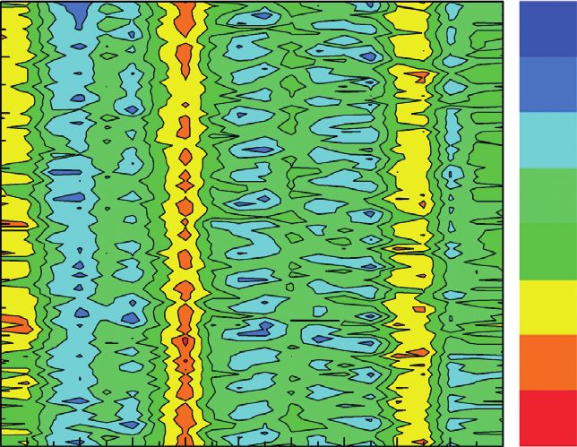
Mathematical Problems in Engineering 9

 Table 1: The main hardware of SIMATIC TDC.
TDC hardware Product model Function
Rack UR5213 21 slots are provided
Central processing unit CPU551 High-performance closed-loop control is achieved
I/O template SM500 Analog and digital input interfaces are provided
Communication template CP51M1 Interrack Ethernet communication and WinCC communication are provided
Program memory module MC500 Storing handlers and hardware configurations are provided

 Table 2: The initial value of coordinated algorithm parameter.
Variable name Variable meaning Variable value
x(0)
 TV Initial point of coordinated algorithm (0, 0, . . . , 0)
εTV Iteration accuracy of coordinated algorithm 1 × 10− 9
T Maximum generation 1000
Mpopulation Population number 100
Pcross Cross probability 0.6
Pmutation Mutation probability 0.07
ai Lower limit of constrained domain −1
bi Upper limit of constrained domain 1

 8.0 Six roll UCM rolling
 mill
 7.5 Ethernet
 Intermediate roll bending
 7.0
 Objective function value

 Intermediate roll
 6.5 shifting
 Shapemeter roll L2
 6.0
 5.5
 Selective work roll cooling
 Work roll tilting
 Work roll bending

 5.0
 4.5 PDA
 Monitoring and diagnostics
 4.0
 3.5
 200 400 600 800
 Iteration number HMI
 SIMATIC TDC
 Coordinated algorithm
 CP50M1
 CP51M1
 CPU551
 CPU551
 CPU551
 SM500
 SM500
 SM500

 GA
 Topkis-veinott algorithm
 Figure 4: The algorithm comparison chart.

 Figure 5: The flatness control system equipment distribution.
roll cooling. SIMATIC TDC controller communicates with
HMI, PDA, and L2 server via Industrial Ethernet. The in-
dependent computer is used for monitoring and diagnostics d1 − d2
of SIMATIC TDC controllers (Table 3). cs � , (16)
 d1
 where cs is compensation efficiency of strip rolling speed. It
3.2. Flatness Control Effect of Different Rolling Speed. represents the compensation efficiency for the flatness de-
When the rolling speed is different, the control effect with viation caused by the speed change. d1 is the average flatness
using the flatness actuator group collaboration strategy is deviation of 910 m/min rolling speed with the conventional
compared with the control effect with using the conventional method. d2 is the average flatness deviation of 1100 m/min
method. The experimental parameter of the flatness control rolling speed with the conventional method.
effect test of different rolling speed is shown in Table 4. The In Figure 8, when the rolling speed is 910 m/min and the
flatness control effect of different rolling speed is shown in control method is changed from conventional model to
Figure 8. collaboration strategy model, the average flatness deviation
 The compensation efficiency of strip rolling speed is as is decreased in every measuring section. The maximum
follows: decreasing magnitude is 3.81 I. It indicates that if the wide
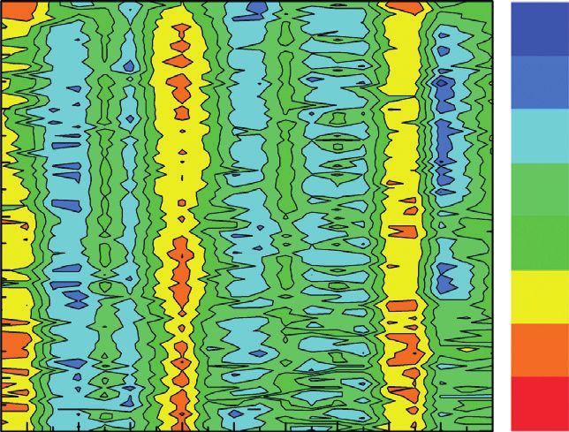
10 Mathematical Problems in Engineering

 Rolling speed: 228 m/min Exit tension: 28.56 kN Rolling force: 9905kN Rolling length: 4892m Strip width: 1200mm Measuring section: 34

 Flatness measurements/flatness distribution/IU Work roll Intermediate Work roll Intermediate
 +40 Rolling force
 bending roll bending tilting roll shifting
 +32
 +26
 +19
 +12
 +6 Flatness
 –15 measurements
 –9
 –22
 –29
 –35 Actual
 –40 –2.26 Max% Max% 24.71
 1 2 3 4 5 6 7 8 9 10 11 12 13 14 15 16 17 18 19 20 21 22 23 24 25 26 27 28 29 30 31 32 33 34 35 36 37 38 value 9905 kN Max% 89.81 –2.74 Max%

 Setpoint 10377 kN –2.42 Max% 89.75 Max% –2.08 Max% 24.68 Max%
 value
 Work roll Intermediate Work roll Intermediate
 Linear learning Quadratic learning bending roll bending tilting roll shifting
 Edge learning library
 library library feedback feedback feedback feedback

 Selective
 cooling

 Cooling valve

 Figure 6: The operation interface of the flatness control system.

 Rolling direction

 Stand 5 Stand 4 Stand 3 Stand 2 Stand 1

 LS5 + LS4 + + LS2 + LS1 +
 X5 (A) X4 X0 WD

 X5 (B) SM TM5 TM4 TM3 TM2 TM1
 Coiler Flying shear + + + + +

 Thickness meter (X) Laser speedometer (LS)

 Weld detector (WD) Tension roller (TM)
 Plate roller (SM)
 Figure 7: The 1450 mm five-stand cold rolling mill production line.

strip is rolled, the control effect of using collaboration effect test of different rolling force is shown in Tables 5 and 6.
strategy model is better than the control effect of using The flatness control effect of different rolling force is shown
conventional model. When the conventional model is used in Figure 9.
and the rolling speed is changed from 1100 m/min to 910 m/ The compensation efficiency of rolling force is as follows:
min, the average flatness deviation is increased in every
measuring section. The maximum increasing magnitude is e1 − e2
 cf � , (17)
3.17 I. It indicates that if the conventional model is used, the e1
control effect of low rolling speed is worse than control effect
 where cf is the compensation efficiency of rolling force. It
of high rolling speed. When the rolling speed is changed
 represents the compensation efficiency for the flatness de-
from 910 m/min to 1100 m/min and the control method is
 viation caused by the change of rolling force. e1 is the average
changed from collaboration strategy model to conventional
 flatness deviation of 8300 kN ∼ 8900 kN with conventional
model, the change of average flatness deviation is small. The
 method. e2 is the average flatness deviation of
maximum changing magnitude is 1.33 I. It indicates that the
 7700 kN ∼ 8300 kN with conventional method.
rolling speed can be compensated by using collaboration
 In Figure 9, when the rolling force is 8300 kN ∼ 8900 kN
strategy model. The maximal compensation efficiency of
 and the control method is changed from conventional model
strip rolling speed is 51.89%.
 to collaboration strategy model, the average flatness devi-
 ation is decreased in every measuring section. The maximum
3.3. Flatness Control Effect of Different Rolling Force. decreasing magnitude is 2.52 I. It indicates that if the strip is
When the rolling force is different, the control effect with rolled in large rolling force, the control effect of using
using the flatness actuator group collaboration strategy is collaboration strategy model is better than the control effect
compared with the control effect with using conventional of using conventional model. When the conventional model
method. The experimental parameter of the flatness control is used and the rolling force is changed from
Mathematical Problems in Engineering 11

 Table 3: The average flatness deviation of different rolling speed.
 Difference between the average flatness Difference between the average flatness Absolute value of difference between the
 deviation of 910 m/min rolling speed deviation of 910 m/min rolling speed average flatness deviation of 910 m/min
Measure with conventional method and the with conventional method and the rolling speed with collaboration strategy
segment average flatness deviation of 910 m/min average flatness deviation of 1100 m/ and the average flatness deviation of
 rolling speed with collaboration min rolling speed with conventional 1100 m/min rolling speed with
 strategy/I method/I conventional method/I
1 3.81 1.95 0.30
2 1.79 1.51 0.28
3 2.13 2.24 0.10
4 1.56 1.11 0.44
5 1.20 1.32 0.11
6 1.82 1.50 0.32
7 1.03 1.59 0.55
8 0.85 0.28 0.56
9 1.62 1.90 0.27
10 1.97 1.47 0.50
11 0.94 1.61 0.67
12 1.32 1.02 0.30
13 1.54 1.98 0.44
14 1.82 1.50 0.32
15 1.00 0.57 0.42
16 1.19 1.99 0.79
17 1.60 2.12 0.52
18 1.83 3.17 1.33
19 1.22 1.52 0.30
20 1.65 0.98 0.67

 Table 4: The experimental parameter of the flatness control effect test of different rolling speed.
Test number Gauge/mm Strip Rolling speed/m/min Strategy
1 2.2 × 1250 ⟶ 0.28 × 1250 DDQ 1100 Conventional method
2 2.2 × 1250 ⟶ 0.28 × 1250 DDQ 910 Collaboration strategy
3 2.2 × 1250 ⟶ 0.28 × 1250 DDQ 910 Conventional method

7700kN–8300 kN to 8300 kN ∼ 8900 kN, the average flatness f1 − f2
deviation is increased in every measuring section. The maxi- cr � , (18)
 f1
mum increasing magnitude is 2.71 I. It indicates that if the
conventional model is used, the control effect of large rolling where cr is the compensation efficiency of rolling reduction.
force is worse than control effect of little rolling force. When the It represents the compensation efficiency for the flatness
rolling force is changed from 7700 kN–8300 kN to deviation caused by the change of the rolling reduction. f1 is
8300 kN ∼ 8900 kN and the control method is changed from the average flatness deviation of 32.96% rolling reduction
conventional model to collaboration strategy model, the with conventional method. f2 is the average flatness devi-
change of average flatness deviation is small. The maximum ation of 15.89% rolling reduction with conventional method
changing magnitude is 1.15 I. It indicates that the rolling force (Table 8).
can be compensated by using collaboration strategy model. The In Figure 10, when the rolling reduction is 32.96 and the
maximal compensation efficiency of rolling force is 42.88%. control method is changed from conventional model to
 collaboration strategy model, the average flatness deviation
 is decreased in every measuring section. The maximum
3.4. Flatness Control Effect of Different Rolling Reduction. decreasing magnitude is 5.89 I. It indicates that if the strip is
When the rolling reduction is different, the control effect rolled in high rolling reduction, the control effect of using
with using the flatness actuator group collaboration strategy collaboration strategy model is better than the control effect
is compared with the control effect with using conventional of using conventional model. When the conventional model
method. The experimental parameter of the flatness control is used and the rolling reduction is changed from 15.89% to
effect test of different rolling reduction is shown in Table 7. 32.96%, the average flatness deviation is increased in every
The flatness control effect of different rolling reduction is measuring section. The maximum increasing magnitude is
shown in Figure 10. 2.93 I. It indicates that if the conventional model is used, the
 The compensation efficiency of rolling reduction is as control effect of high rolling reduction is worse than control
follows: effect of low rolling reduction. When the rolling reduction is
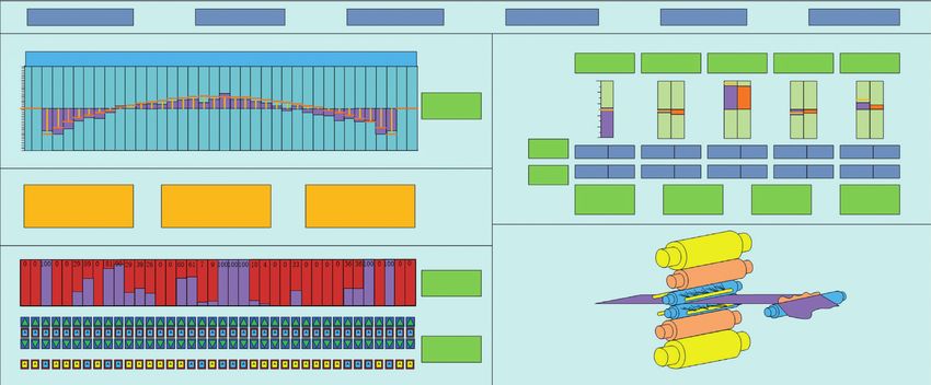
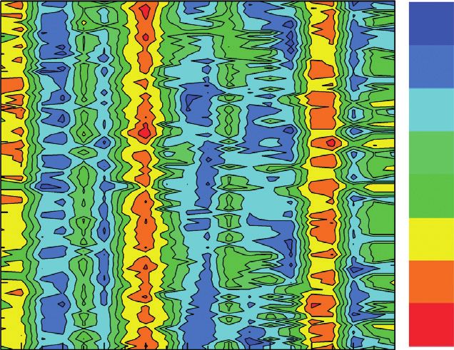
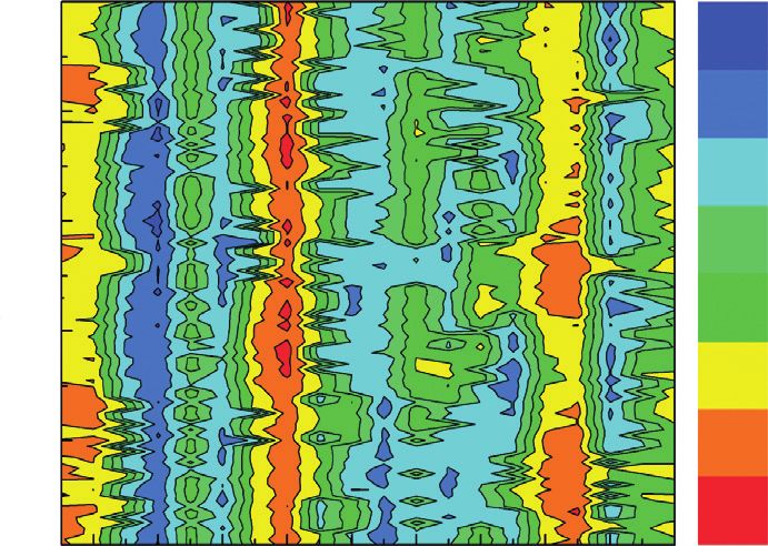
12 Mathematical Problems in Engineering

 800 –15.00
 –15.00
 700 –10.94 15 –10.94
 –6.875
 600 –6.875
 10
 –2.813

 Flatness deviation/I
 Sampling point
 500 –2.813
 5 1.250

 400 1.250 5.313
 0
 9.375
 300 5.313
 –5 13.44
 200 9.375 17.50
 –10 800
 700
 100 13.44 600
 –15 500

 tn
 oi
 2 4 400

 gp
 6 8 300

 in
 17.50
 Meas 10 12 200

 pl
 2 4 6 8 10 12 14 16 18 20

 m
 ure s 14 16 100

 Sa
 Measure segment egme 18
 nt 20

 (a)
 800 –15.00 –15.00

 15 –10.94
 700 –10.94
 –6.875
 600 –6.875 10
 –2.813

 Flatness deviation/I
 Sampling point

 500 –2.813 5 1.250
 5.313
 400 1.250 0
 9.375
 300 5.313 –5 13.44

 200 9.375 –10 800 17.50
 700
 600
 100 13.44 –15 500

 nt
 2 4 400

 oi
 gp
 6 8 300

 in
 17.50 10 12 200

 pl
 Meas 14 16 100

 m
 2 4 6 8 10 12 14 16 18 20 ure s

 Sa
 egme 18
 Measure segment nt 20

 (b)
 800 –17.50
 –17.50
 20
 700 –12.81 –12.81
 15
 600 –8.125 –8.125
 Flatness deviation/I

 10 –3.438
 Sampling point

 500 –3.438
 5 1.250
 400 1.250 5.938
 0
 300 5.938 10.63
 –5
 15.31
 200 10.63 –10
 800 20.00
 –15 700
 100 15.31 600
 500
 nt

 2 4 400
 oi
 gp

 20.00 6 8 300
 in

 2 4 6 8 10 12 14 16 18 20 10 12 200
 pl

 Meas 14 100
 m

 Measure segment ure s 16
 Sa

 egme 18
 nt 20

 (c)

 14

 12

 10
 Flatness deviation/I

 8

 6

 4

 2

 0
 0 5 10 15 20
 Measure segment

 The average flatness deviation of 1100 m/min rolling speed with
 conventional method
 The average flatness deviation of 910m/min rolling speed with
 collaboration strategy
 The average flatness deviation of 910m/min rolling speed with
 conventional method

 (d)

Figure 8: The flatness control effect of different rolling speed. (a) The control effect of 1100 m/min rolling speed with using conventional
model. (b) The control effect of 910 m/min rolling speed with using collaboration strategy. (c) The control effect of 910 m/min rolling speed
with using conventional model. (d) The average flatness deviation of different rolling speed.
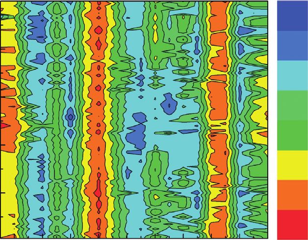
Mathematical Problems in Engineering 13

 Table 5: The experimental parameter of the flatness control effect test of different rolling force.
Test number Gauge/mm Strip Rolling force/kN Strategy
4 3.5 × 1250 ⟶ 0.88 × 1250 SPCC 8300 ∼ 8900 Collaboration strategy
5 3.5 × 1250 ⟶ 0.88 × 1250 SPCC 7700–8300 Conventional method
6 3.5 × 1250 ⟶ 0.88 × 1250 SPCC 8300 ∼ 8900 Conventional method

 Table 6: The average flatness deviation of different rolling force.
 Absolute value of difference between the
 Difference between the average flatness Difference between the average flatness
 average flatness deviation of
 deviation of 8300 kN ∼ 8900 kN rolling deviation of 8300 kN ∼ 8900 kN rolling
 7700kN–8300 kN rolling force with
Measure force with conventional method and the force with conventional method and the
 conventional method and the average
segment average flatness deviation of average flatness deviation of
 flatness deviation of 8300 kN ∼ 8900 kN
 8300 kN ∼ 8900 kN rolling force with 7700 kN ∼ 8300 kN rolling force with
 rolling force with collaboration strategy/
 collaboration strategy/I conventional method/I
 I
1 2.52 2.01 0.51
2 1.33 1.58 0.24
3 2.43 2.01 0.43
4 2.00 1.81 0.18
5 1.23 1.37 0.13
6 1.02 2.17 1.15
7 1.28 1.91 0.62
8 1.59 1.05 0.53
9 2.30 2.06 0.26
10 0.88 0.82 0.05
11 0.93 1.11 0.17
12 0.65 0.67 0.02
13 1.20 1.18 0.01
14 0.99 0.85 0.13
15 1.79 1.74 0.04
16 1.23 0.83 0.39
17 0.94 0.96 0.02
18 2.15 2.71 0.55
19 0.90 1.25 0.34
20 1.61 1.57 0.04

 100 –14.00 –14.00
 15
 –10.38 –10.38
 80 10 –6.750
 Flatness deviation/I

 –6.750
 –3.125
 Sampling point

 –3.125 5 0.5000
 60
 4.125
 0.5000 0
 7.750
 40 4.125 –5 11.38
 7.750 15.00
 –10 100
 20 80
 11.38
 nt

 60
 oi

 2 4 40
 gp

 15.00 6 8
 in

 Meas 10 12 14 20
 pl

 2 4 6 8 10 12 14 16 18 20 ure s
 m

 egme 16 18
 Sa

 Measure segment nt 20

 (a)
 Figure 9: Continued.
14 Mathematical Problems in Engineering

 100 –13.00 –13.00
 15 –9.375
 –9.375
 80 –5.750
 –5.750 10

 Flatness deviation/I
 –2.125

 Sampling point
 60 –2.125 5 1.500

 1.500 5.125
 0
 8.750
 40 5.125
 –5 12.38
 8.750 16.00
 20 –10 100
 12.38 80

 nt
 60

 oi
 2 4

 gp
 16.00 6 8 40

 in
 2 4 6 8 10 12 14 16 18 20 Meas 10 12 14 20

 pl
 ure s

 m
 Measure segment egme 16 18

 Sa
 nt 20

 (b)
 100 –17.50 –17.50
 –13.13 15 –13.13
 80 –8.750
 –8.750 10

 Flatness deviation/I
 –4.375
 Sampling point

 60 –4.375 5 0.000
 0.000 0 4.375
 40 8.750
 4.375 –5
 13.13
 8.750 –10
 17.50
 20 100
 13.13 –15 80

 nt
 60

 oi
 2 4 40

 gp
 17.50 6 8

 in
 2 4 6 8 10 12 14 16 18 20 Meas 10 12 14 20

 pl
 ure s

 m
 Measure segment egme 16 18

 Sa
 nt 20

 (c)

 16

 14

 12
 Flatness deviation/I

 10

 8

 6

 4

 2

 0 5 10 15 20
 Measure segment

 The average flatness deviation of 8300 ~ 8900kN with
 collaboration strategy
 The average flatness deviation of 7700 ~ 8300kN with
 conventional method
 The average flatness deviation of 8300 ~ 8900kN with
 conventional method

 (d)

Figure 9: The flatness control effect of different rolling force. (a) The control effect of 8300 kN ∼ 8900 kN rolling force with using col-
laboration strategy. (b) The control effect of 7700 kN–8300 kN rolling force with using conventional model. (c) The control effect of
8300 kN∼8900 kN rolling force with using conventional model. (d) The average flatness deviation of different rolling force.

 Table 7: The experimental parameter of the flatness control effect test of different rolling reduction.
Test number Gauge/mm Strip Rolling reduction/% Strategy
7 2.5 × 1250 ⟶ 0.58 × 1250 Q195 15.89 Conventional method
8 2.5 × 1250 ⟶ 0.58 × 1250 Q195 32.96 Collaboration strategy
9 2.5 × 1250 ⟶ 0.58 × 1250 Q195 32.96 Conventional method
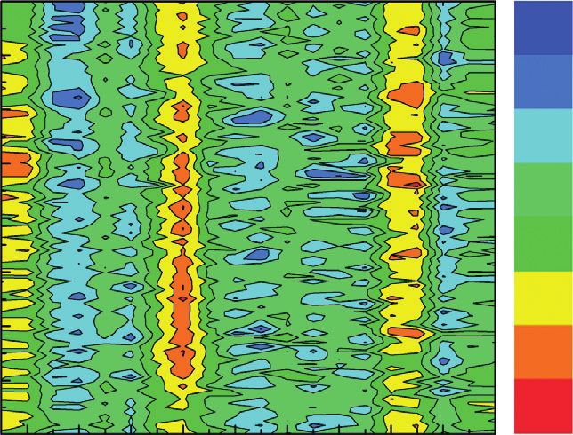
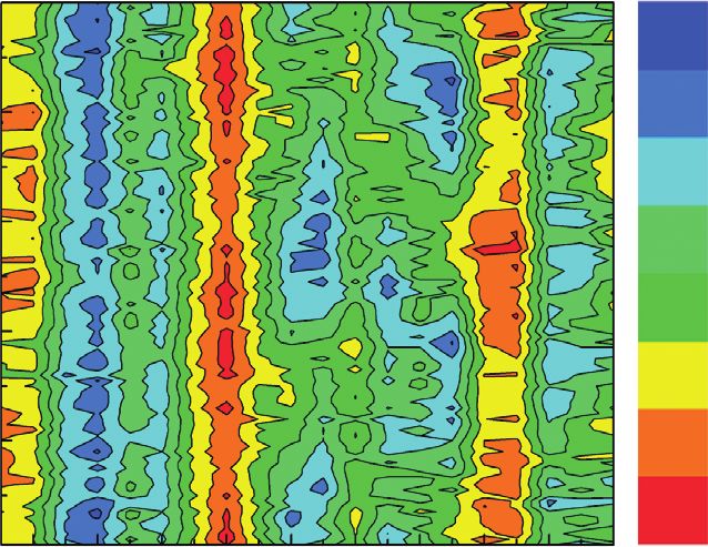
Mathematical Problems in Engineering 15

 100 –17.50 –17.50
 15 –13.13
 –13.13
 80 –8.750
 –8.750 10

 Flatness deviation/I
 –4.375

 Sampling point
 –4.375 5 0.000
 60
 0 4.375
 0.000
 8.750
 40 –5
 4.375 13.13
 –10
 8.750 17.50
 20 100
 –15 80
 13.13

 t
 60

 in
 2 4

 po
 6 8 40

 g
 17.50

 in
 Meas 10 12 14 20

 pl
 2 4 6 8 10 12 14 16 18 20 ure s

 m
 egme 16 18

 Sa
 Measure segment nt 20

 (a)
 100 –12.00 –12.00
 15 –8.500
 –8.500
 80 –5.000
 –5.000 10

 Flatness deviation/I
 –1.500
 Sampling point

 60 –1.500 5 2.000

 2.000 5.500
 0 9.000
 40 5.500
 –5 12.50
 9.000 16.00
 20 100
 12.50 –10 80

 nt
 60

 oi
 2 4 40

 gp
 16.00 6 8
 Meas 10 12 14

 in
 2 4 6 8 10 12 14 16 18 20 20

 pl
 ure s

 m
 Measure segment egme 16 18

 Sa
 nt 20

 (b)
 100 –17.50 –17.50
 20
 –12.81 –12.81
 80 15 –8.125
 –8.125
 Flatness deviation/I

 10 –3.438
 Sampling point

 60 –3.438 1.250
 5
 1.250 5.938
 0
 40 10.63
 5.938 –5
 15.31
 10.63 –10 20.00
 20 100
 15.31 –15 80
 60
 nt

 2 4
 oi

 40
 gp

 20.00 6 8
 Meas 10 12
 in

 2 4 6 8 10 12 14 16 18 20 20
 pl

 ure s 14
 m

 Measure segment egme 16 18
 Sa

 nt 20

 (c)
 20

 18

 16

 14
 Flatness deviation/I

 12

 10

 8

 6

 4

 2

 0 5 10 15 20
 Measure segment

 The average flatness deviation of 15.89% roll reduction with
 conventional method
 The average flatness deviation of 32.96% roll reduction with
 collaboration strategy
 The average flatness deviation of 32.96% roll reduction with
 conventional method

 (d)

Figure 10: The flatness control effect of different rolling reduction. (a) The control effect of 15.89% rolling reduction with using con-
ventional model. (b) The control effect of 32.96% rolling reduction with using collaboration strategy model. (c) The control effect of 32.96%
rolling reduction with using conventional model. (d) The average flatness deviation of different rolling reduction.
16 Mathematical Problems in Engineering

 Table 8: The average flatness deviation of different rolling reduction.
 Difference between the average flatness Difference between the average flatness Absolute value of difference between the
 deviation of 32.96% rolling reduction deviation of 32.96% rolling reduction average flatness deviation of 15.89%
Measure with conventional method and the with conventional method and the rolling reduction with conventional
segment average flatness deviation of 32.96% average flatness deviation of 15.89% method and the average flatness
 rolling reduction with collaboration rolling reduction with conventional deviation of 32.96% rolling reduction
 strategy/I method/I with collaboration strategy/I
1 2.89 2.28 0.61
2 1.32 2.22 0.90
3 2.18 0.88 1.07
4 5.89 1.21 1.31
5 0.37 1.01 0.64
6 2.06 1.57 0.49
7 1.95 2.47 0.51
8 3.76 1.49 1.26
9 1.43 1.63 0.19
10 1.25 0.83 0.42
11 0.52 1.04 0.51
12 1.15 1.04 0.11
13 1.68 0.98 0.70
14 0.79 1.30 0.50
15 0.77 0.32 0.44
16 0.65 0.74 0.08
17 1.16 1.08 0.07
18 2.58 2.93 0.34
19 0.66 0.71 0.04
20 1.61 1.60 0.01

changed from 15.89% to 32.96% and the control method is low rolling speed, large rolling force, and high rolling
changed from conventional model to collaboration strategy reduction by using collaboration strategy.
model, the change of average flatness deviation is small. The
maximum changing magnitude is 1.31 I. It indicates that the Data Availability
rolling reduction can be compensated by using collaboration
strategy model. The maximal compensation efficiency of The data used to support the findings of this study are
rolling reduction is 36.77%. available from the corresponding author upon request.

 Conflicts of Interest
4. Conclusion
 The authors declare that they have no conflicts of interest.
 (1) The flatness actuator group collaboration strategy is
 created on account of the actual flatness condition
 discrimination factor. In the newly raised collabo-
 Acknowledgments
 ration strategy model, the actual flatness situation This study was financially supported by the National Key
 can be calculated and identified. What is more, the R&D Program of China (2017YFB0304100), the National
 overall regulation capacity of flatness adjustment Natural Science Foundation of China (nos. 51804133,
 actuator after the combination is made to match with 51905068, and 61703200), the Natural Science Foundation of
 the flatness defect so that the flatness control system Jiangsu Provincial of China (nos. BK20180977 and
 can give full play to its potential. BK20181024), and the Foundation of Nanjing Institute of
 (2) In online test experiment using collaboration Technology (no. YKJ201867).
 strategy model, a preliminary finding is achieved:
 When the strip rolling speed is increased from References
 910 m/min to 1100 m/min, the maximal compen-
 sation efficiency of rolling speed is 51.89%. When the [1] S. Abdelkhalek, P. Montmitonnet, N. Legrand, and
 rolling force is increased from 7700 kN–8300 kN to P. Buessler, “Coupled approach for flatness prediction in cold
 rolling of thin strip,” International Journal of Mechanical
 8300 kN ∼ 8900 kN, the maximal compensation ef-
 Sciences, vol. 53, no. 9, pp. 661–675, 2011.
 ficiency of rolling force is 42.88%. When the rolling [2] X. Zhang, T. Xu, L. Zhao, H. Fan, and J. Zang, “Research on
 reduction is increased from 15.89% to 32.96%, the flatness intelligent control via GA-PIDNN,” Journal of In-
 maximal compensation efficiency of rolling reduc- telligent Manufacturing, vol. 26, no. 2, pp. 359–367, 2013.
 tion is 36.77%. Thus, it can be seen that the flatness [3] P. Wang, D. Qiao, D. Zhang, J. Sun, and H. Liu, “Optimal
 control effect is improved under rolling conditions of multi-variable flatness control for a cold rolling mill based on
Mathematical Problems in Engineering 17

 a box-constraint optimisation algorithm,” Ironmaking & [20] N. Lu, B. Jiang, and J. Lu, “Data mining-based flatness pattern
 Steelmaking, vol. 43, no. 6, pp. 426–433, 2016. prediction for cold rolling process with varying operating
 [4] K. Prinz, A. Steinboeck, and A. Kugi, “Optimization-based condition,” Knowledge and Information Systems, vol. 41, no. 2,
 feedforward control of the strip thickness profile in hot strip pp. 355–378, 2014.
 rolling,” Journal of Process Control, vol. 64, pp. 100–111, 2018. [21] P.-f. Wang, Y. Peng, H.-m. Liu, D.-h. Zhang, and J.-s. Wang,
 [5] Q.-L. Wang, J. Sun, X. Li, Y.-M. Liu, P.-F. Wang, and “Actuator efficiency adaptive flatness control model and its
 D.-H. Zhang, “Numerical and experimental analysis of strip application in 1250 mm reversible cold strip mill,” Journal of
 cross-directional control and flatness prediction for UCM Iron and Steel Research International, vol. 20, no. 6, pp. 13–20,
 cold rolling mill,” Journal of Manufacturing Processes, vol. 34, 2013.
 pp. 637–649, 2018. [22] L. P. Yang, H. X. Yu, D. C. Wang et al., “Intelligent shape
 [6] S. Voronin, D. Y. Usatyi, V. R. Gasiyarov et al., “Analysis of regulation cooperative model of cold rolling strip and its
 the use of cambered roll with the roll shift system CVC to application,” Steel Research International, vol. 88, no. 7,
 adjust the gap on the hot plate mill,” Russian Internet Journal pp. 1–11, 2017.
 of Industrial Engineering, vol. 3, no. 1, pp. 45–48, 2015. [23] T. Sumeet, T. C. Kevin, and J. D. Louis, “Error modeling for
 [7] X. Ju and R. Mahnken, “Goal-oriented adaptivity for linear surrogates of dynamical systems using machine learning,”
 elastic micromorphic continua based on primal and adjoint International Journal for Numerical Methods in Engineering,
 consistency analysis,” International Journal for Numerical vol. 112, no. 12, pp. 1801–1827, 2017.
 Methods in Engineering, vol. 112, no. 8, pp. 1017–1039, 2017. [24] X.-L. Zhang, L. Cheng, S. Hao, W.-Y. Gao, and Y.-J. Lai, “The
 [8] H. N. Bu, Z. W. Yan, D. H. Zhang, and S. Z. Chen, “Rolling new method of flatness pattern recognition based on GA-
 schedule multi-objective optimizationbased on influence RBF-ARX and comparative research,” Nonlinear Dynamics,
 function for thin gauge steel strip in tandem cold rolling,” vol. 83, no. 3, pp. 1535–1548, 2016.
 Scientia Iranica, vol. 23, no. 6, pp. 2663–2672, 2016. [25] X.-L. Zhang, L. Cheng, S. Hao, W.-Y. Gao, and Y.-J. Lai,
 [9] C.-Y. Jia, T. Bai, X.-Y. Shan, F.-J. Cui, and S.-J. Xu, “Cloud “Optimization design of RBF-ARX model and application
 neural fuzzy PID hybrid integrated algorithm of flatness research on flatness control system,” Optimal Control Ap-
 control,” Journal of Iron and Steel Research International, plications and Methods, vol. 38, no. 1, pp. 19–35, 2017.
 vol. 21, no. 6, pp. 559–564, 2014.
[10] C. Liu, B. Liu, L. Zhao, Y. Xing, C. Ma, and H. Li, “A dif-
 ferential quadrature hierarchical finite element method and its
 applications to vibration and bending of Mindlin plates with
 curvilinear domains,” International Journal for Numerical
 Methods in Engineering, vol. 109, no. 2, pp. 174–197, 2016.
[11] H. Liu, H. T. He, X. Y. Shan et al., “Flatness control based on
 dynamic effective matrix for cold strip mills,” Chinese Journal
 of Mechanical Engineering, vol. 22, no. 2, pp. 287–296, 2009.
[12] H.-M. Liu, X.-Y. Shan, and C.-Y. Jia, “Theory-intelligent
 dynamic matrix model of flatness control for cold rolled
 strips,” Journal of Iron and Steel Research International,
 vol. 20, no. 8, pp. 1–7, 2013.
[13] D. C. Tran, N. Tardif, and A. Limam, “Experimental and
 numerical modeling of flatness defects in strip cold rolling,”
 International Journal of Solids and Structures, vol. 69-70,
 pp. 343–349, 2015.
[14] N. Mathieu, M. Potier-Ferry, and H. Zahrouni, “Reduction of
 flatness defects in thin metal sheets by a pure tension leveler,”
 International Journal of Mechanical Sciences, vol. 122,
 pp. 267–276, 2017.
[15] R. Nakhoul, P. Montmitonnet, and N. Legrand, “Manifested
 flatness defect prediction in cold rolling of thin strips,” In-
 ternational Journal of Material Forming, vol. 8, no. 2,
 pp. 283–292, 2015.
[16] M. Salimi and M. M. Sahebifard, “Optimization of strip profile
 and flatness using hybrid neural-GA algorithm,” Steel Re-
 search International, vol. 81, no. 9, pp. 154–157, 2010.
[17] W. Q. Sun, B. Li, J. Shao et al., “Research on crown & flatness
 allocation strategy of hot rolling mills,” International Journal
 of Simulation Modelling, vol. 15, no. 2, pp. 327–340, 2016.
[18] D. C. Tran, N. Tardif, H. El Khaloui, and A. Limam, “Thermal
 buckling of thin sheet related to cold rolling: latent flatness
 defects modeling,” Thin-Walled Structures, vol. 113,
 pp. 129–135, 2017.
[19] X. Zhang, L. Zhao, J. Zang, H. Fan, and L. Cheng, “Flatness
 intelligent control based on T-S cloud inference neural net-
 work,” Isij International, vol. 54, no. 11, pp. 2608–2617, 2014.
You can also read