Learning to Coordinate via Multiple Graph Neural Networks

Learning to Coordinate via Multiple Graph Neural
 Networks

 Zhiwei Xu, Bin Zhang, Yunpeng Bai, Dapeng Li, and Guoliang Fan

 Institute of Automation, Chinese Academy of Sciences.
 University of Chinese Academy of Sciences School of Artificial Intelligence.
 {xuzhiwei2019, zhangbin2020, baiyunpeng2020, lidapeng2020, guoliang.fan}@ia.ac.cn
arXiv:2104.03503v1 [cs.MA] 8 Apr 2021

 Abstract. The collaboration between agents has gradually become an important topic in
 multi-agent systems. The key is how to efficiently solve the credit assignment problems.
 This paper introduces MGAN for collaborative multi-agent reinforcement learning, a new
 algorithm that combines graph convolutional networks and value-decomposition methods.
 MGAN learns the representation of agents from different perspectives through multiple graph
 networks, and realizes the proper allocation of attention between all agents. We show the
 amazing ability of the graph network in representation learning by visualizing the output of
 the graph network, and therefore improve interpretability for the actions of each agent in the
 multi-agent system.

 Keywords: Multi-Agent Reinforcement Learning · Graph Neural Network · Coordination
 and Control

 1 Introduction

 In the past decade, multi-agent systems (MAS) have received considerable attention from researchers
 due to their extensive application scenarios. The change of the environment is no longer determined
 by a single agent but is the result of the joint actions of all agents in MAS, which results in the
 traditional single-agent reinforcement learning algorithm cannot be directly applied to the case of
 Multi-Agent. In the field of cooperative multi-agent reinforcement learning, since the dimension-
 ality of the joint action space of multi-agents will increase exponentially as the number of agents
 increases, the centralized method of combining multiple agents as a single agent for training cannot
 achieve desired results. In addition, there is a decentralized approach represented by Independent
 Q-Learning (IQL) [20], in which each agent learns independently, using other agents as part of the
 environment, but this method is unstable and easy to overfit. At present, centralized training and
 distributed execution (CTDE) [9] are the most popular learning paradigms, in which we can use
 and share some global information during training to make the distributed execution more effective,
 so as to improve learning efficiency.
 On the one hand, it’s better to learn a centralized action-value function to capture the effects
 of all agents’ actions. On the other hand, such a function is difficult to learn. Even if it can be
 learned, there is no obvious way for us to extract decentralized policy. Facing this challenge, the
 COMA [4] algorithm learns a fully centralized Q-value function and uses it to guide the training
 of decentralized policies in an actor-critic framework. Different from this method, researchers have
 proposed another value-based algorithm. The main idea is to learn a centralized but decomposable
 value function. Both Value-Decomposition Network (VDN) [18] and QMIX [14] adopt this idea.

2 Zhiwei Xu, Bin Zhang, Yunpeng Bai, Dapeng Li, Guoliang Fan

VDN approximates joint action-value function as the linear summation of the individual value
functions obtained through local observations and actions, but in fact, the relationship between
joint action-value and individual action-value is much more complicated than this, besides, VDN
ignores any additional state information available during learning. The QMIX algorithm relaxes the
restriction on the relationship between the whole and the individual. It approximates joint Q-value
function through a neural network and decomposes it into a monotonically increasing function of
all individual values. In addition, there are many excellent works in the field of value function
decomposition, such as QTRAN [16] that directly learn the joint action value function and then fit
residuals with another network.
 The above-mentioned value-decomposition methods have achieved good results in the SMAC [15]
testbed. But it’s worth noting that the aforementioned algorithms mainly focus on the value decom-
position for credit assignment, but the underlying topology between agents in the MAS is not paid
attention to or utilized. When we take this structure into account, a natural idea is to use graph
structure for modeling. For data in an irregular or non-Euclidean domain, graph convolutional net-
works (GCNs) [3, 6, 13, 21, 23–25] can replace traditional convolution operations and perform graph
convolutions by taking the weighted average of a node’s neighborhood information, so as to use
the geometric structure of the graph to learn the embedding feature of each node or the whole
graph. Recently, many graph convolutional networks based on different types of aggregators have
been proposed, and significant results have been obtained on many tasks such as node classification
or graph classification. Since the agents in the MAS can communicate and influence each other,
similar to social networks, some works that combines graph networks and multi-agent reinforcement
learning have appeared. Most of them can be seen as variants that increase the communication be-
tween agents. For example, CommNet [17], BiCNet [12], and DGN [1] all use different convolutional
kernels to process the information transmitted by neighbor agents.
 In this paper, we propose a multi-agent reinforcement learning algorithm based on the CTDE
structure that combines graph convolutional neural networks with value-decomposition method,
namely Multi-Graph Attention Network (MGAN). We establish an undirected graph, and each
agent acts as a node in the graph. Based on this graph, we build multiple graph convolutional
neural networks and the attention mechanism [22] is used in the aggregators. The input of the
network is the individual value function obtained by a single agent, and the output of the network
is the global value function. At the same time, in order to ensure that the local optimal action
is the same as the global optimal action, the MGAN algorithm also satisfies the monotonicity
assumption. Graph convolutional network effectively learns the vector representation of the agents
in MAS, making the efficiency and accuracy of centralized training higher than other algorithms.
Our experiments also show that the MGAN algorithm is superior in performance to the baseline
algorithms, especially in the scenarios of a large number of agents.
Contribution
 – We propose MGAN, a multi-agent reinforcement learning algorithm that combines graph con-
 volutional networks and value-decomposition methods. The graph network is used to make full
 use of the topological structure between agents, thereby increasing the speed of training.
 – The graph networks can learn the vector representation of each agent in the embedding space.
 By visualizing these vectors, we can intuitively understand that all agents are divided into
 several groups at each step, thereby improving interpretability for the agents’ behaviors.
 – We demonstrate through experiments that the proposed algorithm is comparable to the baseline
 algorithms in the SMAC environment. In some scenarios with a large number of agents, MGAN
 significantly outperforms previous state-of-the-art methods.

Learning to Coordinate via Multiple Graph Neural Networks 3

2 Background
2.1 Dec-POMDP
A fully cooperative multi-agent task can be modeled as a decentralized partially observable Markov
decision process (Dec-POMDP) [11] in which each agent only takes a local observation of the
environment. A typical Dec-POMDP can be defined by a tuple G =< S, U, P, Z, r, O, n, γ >. s ∈ S
is the global state of the environment. At each timestep, every agent a ∈ A := {1, ..., n} will choose
an individual action ua ∈ U. The joint action takes the form of u ∈ U ≡ U n . P denotes the
state transition function. All the agents in Dec-POMDP share the same global reward function
r(s, u) : S × U → R. According to the observation function O(s, a) : S × A → Z, each agent a gets
local individual partial observation z ∈ Z. γ ∈ [0, 1) is the discount factor.
 In Dec-POMDP, each agent a has its own action-observation history τa ∈ T ≡ (Z × U). The
policy of each agent a can P be written as πa (ua |τa ) : T × U → [0, 1]. Our aim is to maximize
 ∞
the discounted return Rt = l=0 γ l rt+l . The joint action-value function can be computed by the
following equation: Qπ (st , ut ) = Est+1:∞ ,ut+1:∞ [Rt |st , ut ], where π is the joint policy of all agents.

2.2 Value-Decomposition Multi-Agent RL
In the cooperative multi-agent reinforcement learning problem, one of the most basic solutions is to
learn action-value function of each agent independently. It’s more related to the individual agent’s
observations. However, previous studies indicate that this method is often very unstable and it is
very difficult to design an efficient reward function. By contrast, learning the overall joint reward
function is the other extreme. A key limitation of this method is that the problem of ”lazy agents”
often occurs, i.e., only one agent active and the other being ”lazy”.
 To solve this issue, many researchers have proposed various methods lying between the extremes
of independent Q-learning and centralized Q-learning, such as VDN, QMIX and QTRAN, which try
to achieve automated learning decomposition of joint value function by the CTDE method. These
value-decomposition methods are based on the Individual-Global-Max (IGM) [16] assumption that
the optimality of each agent is consistent with the optimality of all agents. The equation that
describes IGM is as follows:
  
 arg maxu1 Q1 (τ1 , u1 )
 arg max Qtot (τ , u) =  ..
 ,
  
 u .
 arg maxun Qn (τn , un )

where Qtot is global action-value function and Qa is the individual ones.
 VDN assumes that the joint value function is linearly decomposable. Each agent learns the
additive value function independently. VDN aims to learn the optimal linear value decomposition
from the joint action-value function to reflect the value function of each agent. The sum Qtot of all
individual value functions is given by
 n
 X
 Qtot (s, ua ) = Qa (s, ua ).
 a=1

By this method, spurious rewards can be avoided and training is easier for each agent. However,
because the additivity assumption used by VDN is too simple and there are only few applicable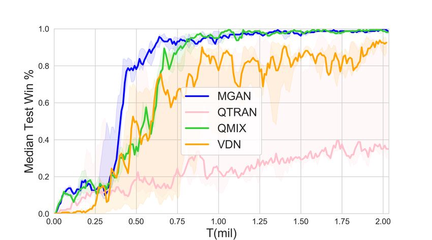

4 Zhiwei Xu, Bin Zhang, Yunpeng Bai, Dapeng Li, Guoliang Fan

scenarios, a nonlinear global value function is proposed in QMIX. QMIX introduces a new type of
value function module named mixing network. In order to satisfy the IGM assumption, it is assumed
that the joint action-value function Qtot is monotonic to the individual action-value function Qa :

 ∂Qtot (τ , u)
 ≥ 0, ∀a ∈ {1, . . . , n}.
 ∂Qa (τa , ua )

 Furthermore, QTRAN uses a new approach that can relax the assumption. However, several
studies have indicated that the actual performance of the QTRAN is not very good because of its
relaxation.

2.3 Graph Convolutional Networks
Convolutional graph neural network, as a kind of graph neural network, is often used to process
data of molecules, social, biological, and financial networks. Convolutional graph neural networks
fall into two categories, spectral-based and spatial-based. Spectral-based methods analyze data
from the perspective of graph signal processing. The spatial-based convolutional graph neural net-
work processes the data of graph by means of information propagation. The emergence of graph
convolutional network has well unified these two methods.
 Let G = (V, E) be a graph. Each node v ∈ V in the graph has its own feature, which is denoted
 (0)
as hv . Assuming that a graph convolutional network has a K-layers structure, then the hidden
output of the k-th layer of the node v is updated as follows:

 a(k)
 v = AGGREGAT E
 (k)
 ({h(k−1)
 u |u ∈ N (v)}),
 (1)
 h(k)
 v = COM BIN E
 (k) (k)
 (av , h(k−1)
 v ),

where COM BIN E is often a 1-layer MLP, and N is the neighborhood function to get immediate
neighbor nodes. Each node v ∈ V aggregates the representations of the nodes in its immediate
neighborhood to get a new vector representation. With the introduction of different AGGREGAT E
functions, various variants of the graph convolutional network have obtained desired results on
some datasets. For example, in addition to the most common mean aggregators, Graph Attention
Network (GAT) [23] uses attention aggregators and Graph Isomorphism Network (GIN) [24] uses
sum aggregators, both of which have achieved better results.

3 MGAN
In this section, we will propose a new method called MGAN. By constructing multiple graph
convolutional networks at the same time, each graph convolutional network has its own unique
insights into the graphs composed of agents. This algorithm can not only make full use of the
information of each agent and the connections between agents, but also improve the robustness of
the performance.

3.1 Embedding generation via graph networks
First, we need to construct all agents as a graph G = (V, E), where each agent a can be seen as a
node in the graph v ∈ V , i.e., agent a and node v has a one-to-one correspondence. We define the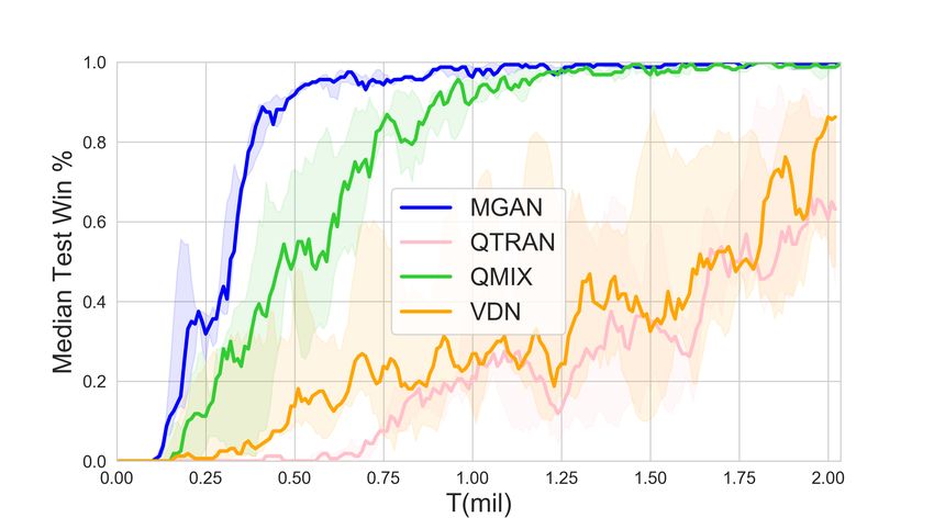

Learning to Coordinate via Multiple Graph Neural Networks 5

 ( , )

 + 
 
 |⋅|
 
 g = ෍
 
 , 
 ( ,⋅)
 =1

 SOFTMAX , , 
 MGAN MIXING NETWORK
 Transform Layer MLP
 AGGREGATE & COMBINE
 ℎ −1 ℎ 
 1 ( 1 , 1 ) ( , ) GRU

 AGGREGATE & COMBINE

 AGENT 1 ⋯ AGENT N MLP

 ( 1 , 1 ) ( , )
 ( , )

 Fig. 1. The overall architecture of MGAN.

neighborhood function N to get the immediate neighbor nodes of the specified node. The edge euv
between any two nodes in the graph is defined as:
 (
 1, if u ∈ N (v) or v ∈ N (u)
 euv = (2)
 0, otherwise

and according to this definition, we get the adjacency matrix E ∈ Rn×n . In the reinforcement
learning tasks, the adjacency matrix often indicates whether the agents are visible or whether they
can communicate with each other. Each node v has its own feature hv .
 Then we build a two-layer graph convolutional network to learn the embedding vector of
each agent. To build a graph convolutional network, we need to define the AGGREGAT E and
COM BIN E functions mentioned by Equation (1). Considering the actual situation, agents often
need to pay special attention to a few of all other agents in the real tasks. So mean aggregators are
often not qualified for this task. We adopted a simplified dot-product attention mechanism to solve
this problem. The vector av obtained by the node v through the attention aggregate function can
be expressed as:
 av = AGGREGAT E({hu |u ∈ N (v)})
 X exp((hv )T · (hu ))
 = P T
 · hu .
 u exp((hv ) · (hu ))
 u∈N (v)

Then av needs to be entered into the COM BIN E function. It can be clearly seen that the embed-
ding vectors obtained after the AGGREGAT E function processing loses the original characteristics
of the node itself, i.e., the feature of the node is over smooth, and the characteristic information of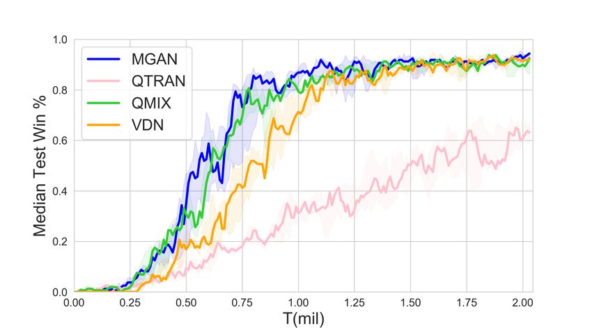

6 Zhiwei Xu, Bin Zhang, Yunpeng Bai, Dapeng Li, Guoliang Fan

the node itself is lacking. Therefore, we define the next layer’s representation h0v of the node v i.e.
output by the COM BIN E function as:

 h0v = COM BIN E(av ) = ReLU (M LP (CON CAT (av , hv )))

This step completes the nonlinear transformation of the features obtained after the node v aggre-
gates its neighbor nodes. Note that the MLP in the COM BIN E function of each layer is shared
for each node. Similar to the simplified JK-Net [25], the original feature hv is concatenated with
the aggregate feature to ensure that the original node information will not be lost. From another
perspective, this is very similar to ResNet [8].

3.2 MGAN Mixing Network

Each agent corresponds to a DRQN [7] network to learn individual action-value Qa , where a ∈
{1, . . . , n}. We have defined the graph convolutional network used to obtain the embedding vector
of the agent, and then we will explain how to construct the network fitting joint action value
function Qtot . The embedding vector obtained through graph convolutional network is input into a
fully connected layer neural network, which we call a transform layer, so that the embedding vector
of each node v is transformed into a scalar cv through affine transformation. The joint action-value
function obtained by this graph convolutional network can be obtained by the following equation:
 n
 X exp(ca )
 (Qa · P ),
 a=1 v∈V exp(cv )

which connects the vectors output by the graph networks with the individual action-values through
dot multiplication.
 Inspired by the multi-head attention mechanism, we propose to use multiple graph convolutional
networks to jointly learn the embedding representation of nodes. Multiple graphs allow the model
to jointly attend to information from different embedding spaces. Multiple graph convolutional
networks share a transform layer. We set the number of graph convolutional networks to G. Thus,
the following equation of the value function corresponding to each graph convolutional network is
obtained:
 n
 X exp(cg,a )
 Qg = (Qa · P ), ∀g ∈ {1, . . . , G}.
 a=1 v∈V exp(cg,v )

where cg,v is the scalar output by the v-th node in the g-th graph convolutional network after the
transform layer.
 VDN obtains the global action-value by simply summing the individual action-values of all
agents. And QMIX uses multiple hypernetworks [5], inputs state s, and outputs network weight pa-
rameters to construct a Mixing Network. It should be noted that in order to satisfy the monotonicity
assumption proposed by QMIX, the network weight parameters output by hypernetworks are all
positive. Our weighted linear factorization lies between the two and has a stronger representational
capability for the joint value function than VDN while keeping a linear decomposition structure.
This is because we only use hypernetworks to generate a layer of mixing network to linearly combine
multiple Qg . The entire network framework of the MGAN algorithm is shown in the Figure 1.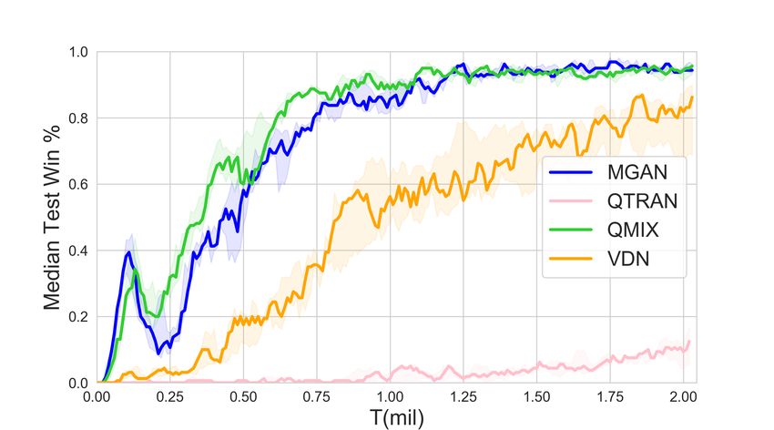

Learning to Coordinate via Multiple Graph Neural Networks 7

3.3 Loss Function

MGAN is the same as other recently proposed MARL algorithms in that they are all trained
end-to-end. The loss function is set to TD-error, which is the same as the traditional value-based
reinforcement learning algorithm [19]. We denote the parameters of all neural networks as θ and
MGAN is trained by minimizing the following loss function:

 L(θ) = (ytot − Qtot (τ , u|θ))2 ,

where ytot is the target joint action-value function and y( tot) = r + γ maxu0 Qtot (τ 0 , u0 |θ− ). θ− are
the parameters of the target network.

 Table 1. Maps in different scenarios.

 Name Ally Units Enemy Units Name Ally Units Enemy Units
 2 Stalkers 2 Stalkers 3 Stalkers 3 Stalkers
 2s3z 3s5z
 3 Zealots 3 Zealots 5 Zealots 5 Zealots
 1 Colossus 1 Colossus
 1c3s5z 3 Stalkers 3 Stalkers 8m vs 9m 8 Marines 9 Marines
 5 Zealots 5 Zealots
 1 Medivac 1 Medivac
 2c vs 64zg 2 Colossi 64 Zerglings MMM 2 Marauders 2 Marauder
 7 Marines 7 Marines
 1 Medivac 1 Medivac
 27m vs 30m 27 Marines 30 Marines MMM2 2 Marauders 3 Marauder
 7 Marines 8 Marines
 25m 25 Marines 25 Marines 25m modified 25 Marines 25 Marines
 4 Banelings 4 Banelings
 bane vs bane so many banelings 7 Zealots 32 Banelings
 20 Zerglings 20 Zerglings

4 Experiment

In this section we will evaluate MGAN and other baselines in the Starcraft II decentralized mi-
cromanagement tasks. In addition, to illustrate the representation learning capacity of the graph
networks, the visualization of the output of the graph network was performed. We can intuitively
understand the motivation of the agents’ decision from the output of the graph neural network.

4.1 Settings

We use SMAC as the testbed because SMAC is a real-time simulation experiment environment
based on Starcraft II. It contains a wealth of micromanagement tasks with varying levels of dif-
ficulty. Recently, it has gradually become an important platform for evaluating the coordination

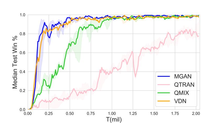
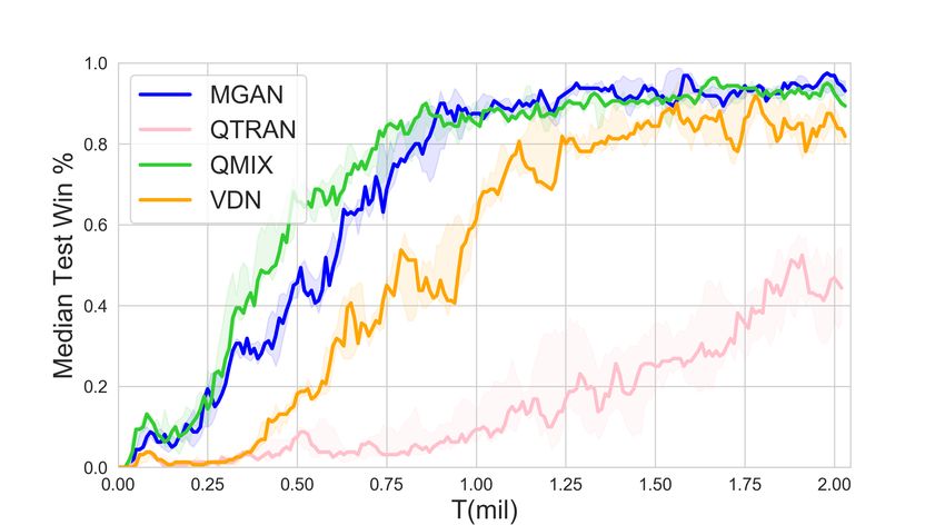
8 Zhiwei Xu, Bin Zhang, Yunpeng Bai, Dapeng Li, Guoliang Fan

 (a) 2s3z (b) 3s5z (c) 1c3s5z (d) 8m vs 9m

 (e) 2c vs 64zg (f) MMM (g) 27m vs 30m (h) MMM2

 (i) 25m (j) 25m modified (k) bane vs bane (l) so many baneling

 Fig. 2. Overall results in different scenarios.

capabilities of agents. The scenarios in SMAC include challenges such as asymmetric, heteroge-
neous, and a large number of agents. We selected more representative scenarios such as 1c3s5z,
3s5z, 2c vs 64zg, MMM2, bane vs bane and so on. Besides, in order to be able to more conveniently
show MGAN’s understanding of the agent in decision-making, we have also introduced a new sce-
nario 25m modified, which is modified on the basis of the 25m scenario. The distribution of agents
in the 25m modified scenario is more dispersed, which makes collaboration more difficult than the
original 25m scenario. The detailed information of all scenarios is shown in the Table 1.
 Our experiment is based on Pymarl [15]. We set the hyperparameters of QMIX and VDN to the
default in Pymarl. The version of the Starcraft II is 4.6.2(B69232) in our experiments. The feature
of each node in the graph network is initialized as its local observation in our proposed MGAN.
And according to Equation (2), the adjacency matrix E is given by:
 (
 1, if u is alive and v is alive
 euv = ∀euv ∈ E.
 0, otherwise

 The number of graph networks G is set to 4, and the other settings are the same as those of other
baselines. We run each experiment 5 times independently to alleviate the effects of accidents and
outliers. Depending on the complexity of the experimental scenario, the duration of each experiment
ranges from 5 to 14 hours. Experiments are carried out on Nvidia GeForce RTX 3090 graphics
cards and Intel(R) Xeon(R) Platinum 8280 CPU. The model is evaluated every 10,000 steps in the
experiment, i.e., 32 episodes are run and the win rate is recorded. The agents follow a completely
greedy strategy during evaluation.

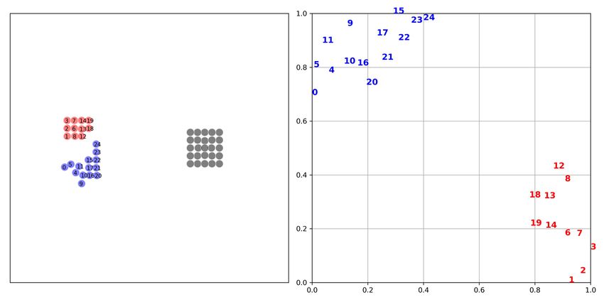
Learning to Coordinate via Multiple Graph Neural Networks 9

4.2 Validation

Figure 2 shows the performance results of MGAN and other baselines in different scenarios. The
solid line represents the median win ratio of the five experiments. The 25-75% percentiles of the win
ratios are shaded. It can be observed that in some scenarios with a large number of agents, MGAN
far exceeds other algorithms in performance. Especially in bane vs bane, MGAN quickly reached
convergence. In other scenarios, MGAN is still comparable to other popular algorithms.

 (a) 2nd step on 25m scenario (b) 6th step on 25m scenario

 (c) 1st step on 25m modified scenario (d) 8th step on 25m modified scenario

Fig. 3. The agents location map at specific step (left) and the corresponding 2D t-SNE embedding of
agents’ internal states output by one of graph convolutional networks (right). Gray dots in location map
represent the enemy agents and color dots denote the agents controlled by MGAN. Each number in 2D
t-SNE embedding corresponds to each color dot in the location map one by one.

 Table 2 shows the median test win rate of different algorithms. As follows from Figure 2 shown
above, it can be seen intuitively that MGAN performs well in hard and super hard scenarios such
as MMM2, bane vs bane and 27m vs 30m.

4.3 Graph Embedding and Weight Analysis

In order to understand the working principle of MGAN and explore the reasons for its effect
improvement, we visualized the embedding vectors output by the graph network and the scalar
weights output by the transform layer. We think these two provide an explanatory basis for the
agents’ actions.
 We choose the 25m and its variant 25m modified scenario with a large number of agents, and
show the positions of the agents at each step in the task as a scatter diagram. Meanwhile, t-SNE [10]

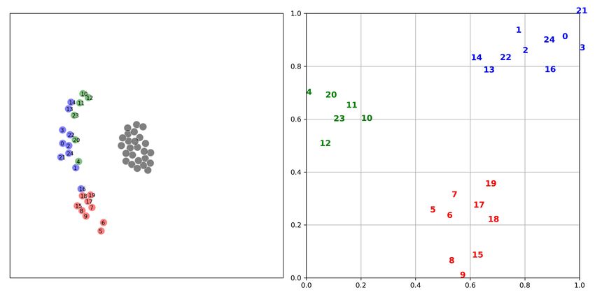
10 Zhiwei Xu, Bin Zhang, Yunpeng Bai, Dapeng Li, Guoliang Fan

 (a) The health values in one episode (b) The weight values in one episode

 Fig. 4. The health values and the weight values on 25m scenario.

 Table 2. Median performance of the test win percentage in different scenarios.

 Scenario MGAN QTRAN QMIX VDN Scenario MGAN QTRAN QMIX VDN
 2s3z 98 93 98 97 3s5z 97 13 96 87
 1c3s5z 96 53 95 88 8m vs 9m 95 65 92 92
 2c vs 64zg 77 9 64 41 MMM 98 85 99 98
 27m vs 30m 44 10 30 16 MMM2 90 0 62 1
 25m 100 40 100 94 25m modified 100 67 100 87
 bane vs bane 100 100 99 82 so many baneling 100 99 99 97

and MeanShift [2] clustering methods are performed on the graph embedding vector corresponding
to each agent in each step, and the corresponding relationship between the position of the agent
and the clustering result can be clearly found. This is illustrated in Figure 3.
 In the 25m scenario, the key to victory is that our agents can form an arc that surrounds the
enemy agents. At the beginning of the episode, all agents gathered together. From the results of
dimensionality reduction and clustering of embedding vectors, it can be found that the agents are
divided into two groups, one group moves upward and the other moves downward. In the middle of
the episode, in order to form a relatively concentrated line of fire, the agents was divided into three
parts and moved in three directions respectively. In the 25m modified scenario, the agents also need
to form the same arc, so the leftmost group of agents needs to move to the right, and the leftmost
group of agents needs to move to the left to rendezvous with other agents. And in the middle of the
episode, it will still be divided into three parts similar to the 25m scenario. The finding was quite
surprising and suggests that agents in the same subgroup can act together.
 For the visualization of the weights, we still use the 25m scenario for verification. The figure
shows the change in the health values of the agents in an episode and the change in the weights of
each agent corresponding to the four graph networks. As can be seen from Figure 4, although the
values of the weights given by each graph network is not the same, they all have a relationship with
the health values of the agents. For example, Graph network 1 believes that agents with drastic
changes in health values are the most important ones, while Graph network 2 believes that agents
with more health values are the most important. On the contrary, Graph network 3 and Graph

Learning to Coordinate via Multiple Graph Neural Networks 11

network 4 pay more attention to agents whose health values are zero. We guess that this is because
these agents cause harm to the enemy and therefore pay more attention.
 Through the analysis, we have concluded that the graph network can learn the characteristics
of each agent well, and this provides basis for our understanding of the actions of the agents, which
improves the interpretability of the motivation of the agents.

5 Conclusion
In this paper, we propose a MARL algorithm called MGAN that combines graph network and
value-decomposition. From the outcome of our experiments it is possible to conclude that MGAN
is comparable to the common baseline, especially in scenarios with a large number of agents. The
figures obtained by visualization indicate that the performance improvement is brought about by
the graph networks. The findings suggest that this method could also be useful for the works to
understand how agents make decisions and what roles they play.
 Since MGAN still needs to satisfy the IGM assumption, in our future research we intend to
concentrate on how to relax the restrictions of the mixing networks. On the basis of the promising
findings presented in this paper, work on the remaining issues is continuing and will be presented
in future papers.

References
 1. Böhmer, W., Kurin, V., Whiteson, S.: Deep coordination graphs. ArXiv abs/1910.00091 (2020)
 2. Comaniciu, D., Meer, P.: Mean shift: A robust approach toward feature space analysis. IEEE Trans.
 Pattern Anal. Mach. Intell. 24, 603–619 (2002)
 3. Defferrard, M., Bresson, X., Vandergheynst, P.: Convolutional neural networks on graphs with fast
 localized spectral filtering. In: NIPS (2016)
 4. Foerster, J.N., Farquhar, G., Afouras, T., Nardelli, N., Whiteson, S.: Counterfactual multi-agent policy
 gradients. In: AAAI (2018)
 5. Ha, D., Dai, A.M., Le, Q.V.: Hypernetworks. ArXiv abs/1609.09106 (2017)
 6. Hamilton, W.L., Ying, Z., Leskovec, J.: Inductive representation learning on large graphs. In: NIPS
 (2017)
 7. Hausknecht, M.J., Stone, P.: Deep recurrent q-learning for partially observable mdps. In: AAAI Fall
 Symposia (2015)
 8. He, K., Zhang, X., Ren, S., Sun, J.: Deep residual learning for image recognition. 2016 IEEE Conference
 on Computer Vision and Pattern Recognition (CVPR) pp. 770–778 (2016)
 9. Lowe, R., Wu, Y., Tamar, A., Harb, J., Abbeel, P., Mordatch, I.: Multi-agent actor-critic for mixed
 cooperative-competitive environments. In: NIPS (2017)
10. Maaten, L.V.D., Hinton, G.E.: Visualizing data using t-sne. Journal of Machine Learning Research 9,
 2579–2605 (2008)
11. Oliehoek, F.A., Amato, C.: A concise introduction to decentralized pomdps. In: SpringerBriefs in In-
 telligent Systems (2016)
12. Peng, P., Wen, Y., Yang, Y., Yuan, Q., Tang, Z., Long, H., Wang, J.: Multiagent bidirectionally-
 coordinated nets: Emergence of human-level coordination in learning to play starcraft combat games.
 arXiv: Artificial Intelligence (2017)
13. Perozzi, B., Al-Rfou, R., Skiena, S.: Deepwalk: online learning of social representations. Proceedings of
 the 20th ACM SIGKDD international conference on Knowledge discovery and data mining (2014)
14. Rashid, T., Samvelyan, M., Witt, C.S., Farquhar, G., Foerster, J.N., Whiteson, S.: Qmix: Monotonic
 value function factorisation for deep multi-agent reinforcement learning. ArXiv abs/1803.11485 (2018)

12 Zhiwei Xu, Bin Zhang, Yunpeng Bai, Dapeng Li, Guoliang Fan

15. Samvelyan, M., Rashid, T., Witt, C.S., Farquhar, G., Nardelli, N., Rudner, T.G.J., Hung, C.M., Torr,
 P., Foerster, J.N., Whiteson, S.: The starcraft multi-agent challenge. ArXiv abs/1902.04043 (2019)
16. Son, K., Kim, D., Kang, W., Hostallero, D., Yi, Y.: Qtran: Learning to factorize with transformation
 for cooperative multi-agent reinforcement learning. ArXiv abs/1905.05408 (2019)
17. Sukhbaatar, S., Szlam, A., Fergus, R.: Learning multiagent communication with backpropagation. In:
 NIPS (2016)
18. Sunehag, P., Lever, G., Gruslys, A., Czarnecki, W., Zambaldi, V., Jaderberg, M., Lanctot, M., Son-
 nerat, N., Leibo, J.Z., Tuyls, K., Graepel, T.: Value-decomposition networks for cooperative multi-agent
 learning. ArXiv abs/1706.05296 (2018)
19. Sutton, R., Barto, A.: Reinforcement learning: An introduction. IEEE Transactions on Neural Networks
 16, 285–286 (2005)
20. Tampuu, A., Matiisen, T., Kodelja, D., Kuzovkin, I., Korjus, K., Aru, J., Aru, J., Vicente, R.: Multiagent
 cooperation and competition with deep reinforcement learning. PLoS ONE 12 (2017)
21. Thekumparampil, K.K., Wang, C., Oh, S., Li, L.: Attention-based graph neural network for semi-
 supervised learning. ArXiv abs/1803.03735 (2018)
22. Vaswani, A., Shazeer, N., Parmar, N., Uszkoreit, J., Jones, L., Gomez, A.N., Kaiser, L., Polosukhin, I.:
 Attention is all you need. ArXiv abs/1706.03762 (2017)
23. Velickovic, P., Cucurull, G., Casanova, A., Romero, A., Liò, P., Bengio, Y.: Graph attention networks.
 ArXiv abs/1710.10903 (2018)
24. Xu, K., Hu, W., Leskovec, J., Jegelka, S.: How powerful are graph neural networks? ArXiv
 abs/1810.00826 (2019)
25. Xu, K., Li, C., Tian, Y., Sonobe, T., Kawarabayashi, K., Jegelka, S.: Representation learning on graphs
 with jumping knowledge networks. In: ICML (2018)