Estimation of stride by stride spatial gait parameters using inertial measurement unit attached to the shank with inverted pendulum model - Nature
←
→
Page content transcription
If your browser does not render page correctly, please read the page content below
www.nature.com/scientificreports
OPEN Estimation of stride‑by‑stride
spatial gait parameters using
inertial measurement unit attached
to the shank with inverted
pendulum model
Yufeng Mao1, Taiki Ogata1*, Hiroki Ora1, Naoto Tanaka2 & Yoshihiro Miyake1
Inertial measurement unit (IMU)-based gait analysis systems have become popular in clinical
environments because of their low cost and quantitative measurement capability. When a shank is
selected as the IMU mounting position, an inverted pendulum model (IPM) can accurately estimate
its spatial gait parameters. However, the stride-by-stride estimation of gait parameters using one
IMU on each shank and the IPMs has not been validated. This study validated a spatial gait parameter
estimation method using a shank-based IMU system. Spatial parameters were estimated via the
double integration of the linear acceleration transformed by the IMU orientation information. To
reduce the integral drift error, an IPM, applied with a linear error model, was introduced at the mid-
stance to estimate the update velocity. the gait data of 16 healthy participants that walked normally
and slowly were used. The results were validated by comparison with those extracted from an optical
motion-capture system; the results showed strong correlation (r > 0.9) and good agreement with the
gait metrics (stride length, stride velocity, and shank vertical displacement). In addition, the biases
of the stride length and stride velocity extracted using the motion capture system were smaller in the
IPM than those in the previous method using the zero-velocity-update. The error variabilities of the
gait metrics were smaller in the IPM than those in the previous method. These results indicated that
the reconstructed shank trajectory achieved a greater accuracy and precision than that of previous
methods. This was attributed to the IPM, which demonstrates that shank-based IMU systems with
IPMs can accurately reflect many spatial gait parameters including stride velocity.
In recent years, many studies have focused on the development of an inertial measurement unit (IMU) equipped
with an accelerometer, gyroscope sensor, and magnetometer for a gait analysis system that can provide quantita-
tive gait parameters such as stride length, velocity, gait cycle. Compared to the golden standard for gait analysis—a
motion capture system and instrumented walkways—the IMU-based system is cost effective, lightweight, and
versatile, which are suitable characteristics for clinical and residential a pplications1. In particular, the inverted
pendulum model (IPM) is considered useful for estimating spatial gait parameters such as stride length from
acceleration and angular velocities measured by the IMU2,3. However, the step-by-step accuracy of the spatial
parameters estimated using the IMU data and IPM model has not been validated thus far.
Kinematics information in the gait cycle is a component of gait considered in clinical gait a nalyses4. For
example, variability in stride length can be used to assess the progression of Parkinson’s disease (PD)5, and
stride velocity can be used to predict the risk of adverse events in the elderly6. To estimate spatial gait parameters
from acceleration and angular velocities measured by the IMU, the previous studies implemented a segmenta-
tion algorithm7–10. Integral computations for spatial parameter estimation are reset at each segmentation point,
which reduces errors caused by the measurement noise. The implementation details of these algorithms depend
on the attachment position of the IMU because different positions produce different signal characteristics and
different assumptions need to be considered to improve estimation accuracy. A wide selection of attachment
1
Department of Computer Science, Tokyo Institute of Technology, Kanagawa 226‑8503, Japan. 2Department
of Systems and Control Engineering, Tokyo Institute of Technology, Kanagawa 226‑8503, Japan. *email:
ogata@c.titech.ac.jp
Scientific Reports | (2021) 11:1391 | https://doi.org/10.1038/s41598-021-81009-w 1
Vol.:(0123456789)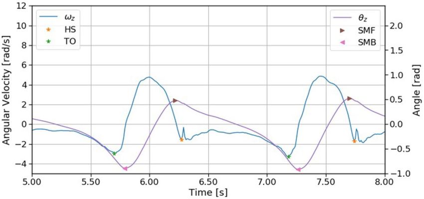
www.nature.com/scientificreports/
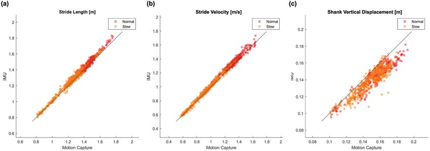
Figure 1. Scatter plots of (a) stride length, (b) stride velocity, and (c) shank vertical displacement extracted
from the proposed method and motion capture system. Each dot indicates the value in one stride. The black line
shows the best fit line.
positions for the IMUs involved bilateral shanks7,11, bilateral insteps12–15, and bilateral heels16,17. In terms of
ensuring attachment stability, the shank position seems to be a good choice because the soft tissue of the lower
shank has less movement than that at the other positions18. Further, when the IMU is fixed to the heel or instep
position on footwear, the moving artifact of the footwear affects the estimation accuracy. However, compared
to the heel or instep attachment positions closer to the ground, the shank position has room for improvement
in terms of estimating spatial parameters such as stride length and stride velocity. The shank-based method can
be used to obtain reliable gait parameters and visualise the 3D-trajectory of each s tride19,20. In a previous study,
zero-velocity-update (ZUPT) was introduced, which re-initialises the integrated velocity to zero at the segmenta-
tion point (mid-stance). However, the shank possesses a small velocity at the mid-stance2, which results in the
error being included in the estimated spatial gait parameters. Instead of assuming the velocity at the mid-stance
to be zero, the inverted pendulum model (IPM)2,3, which considers the IMU movement at the mid-stance as
a circular motion in the sagittal plane and estimates the velocity using angular velocity has the potential to
provide a more accurate result. In fact, Wu et al. showed that the total error of the walking distance estimated
using shank-mounted IMUs and an IPM was smaller than that estimated using the same IMUs and a ZUPT19.
However, it remains unclear if stride-by-stride estimation using shank-mounted IMUs and the IPM is superior
to that using ZUPT. As mentioned above, some variability in the spatial gait parameters is important for the gait
assessment of people with gait disorders, and to investigate such variability in gait parameters, stride-by-stride
estimation of gait parameters is necessary. This study aimed to validate the stride-by-stride estimation method
for spatial gait parameters using shank-mounted IMUs and the IPM. In addition, we investigated whether the
stride-by-stride estimation of the spatial gait parameters using the IPM was superior to that using the ZUPT.
A modified IPM that considered the posture of the IMU for shank trajectory estimation was implemented. For
evaluating the proposed method, we performed a concurrent validation experiment using an optical motion
capture system with a high spatial resolution. Next, we compared the proposed method to a ZUPT method to
investigate whether the IPM improved the accuracy of the stride-by-stride estimation. We used a previously
reported method20 as the ZUPT method because this method had been evaluated for stride-by-stride spatial
gait parameters.
Results
All 16 participants completed both tasks; the data for the normal speed task of one of the participants could not
be analysed because of synchronisation issues (the motion capture system did not capture the stamp event), and
therefore, it was excluded. The motion capture system suffered from loss of data because of the reflective mark-
ers; these invalid data were excluded, and a total of 695 strides were extracted from the motion capture system,
with 283 strides for the normal speed task and 412 strides for the slower speed task.
First, we validated the proposed method compared to the results from the motion capture system. Fig-
ure 1 shows scatter plots for the stride length, stride velocity, and shank vertical displacement between the data
extracted from the proposed method and those obtained from the motion capture system. The stride length and
velocity decreased when the participants walked slowly. Pearson’s correlation coefficient and the error distribution
are summarised in Table 1. All parameters achieve high correlation with Pearson correlation coefficient r > 0.90.
Thus, the proposed method estimated the parameters appropriately.
Second, we investigated whether the proposed method estimated the parameters more accurately than the
previous method. The Bland–Altman plots for the parameters estimated using the proposed method and a previ-
ous method are shown in Fig. 2. The biases of stride length, stride velocity, and shank vertical displacement for
the proposed and previous methods were 0.006 m and −0.059 m, 0.007 m/s and −0.047 m/s, and −0.010 m and
−0.009 m, respectively. The stride length and stride velocity estimated using the proposed method achieved a
very small bias compared with those estimated using the previous method. The 95% confidence intervals of stride
length, stride velocity, and shank vertical displacement for the proposed and previous methods were 0.099 m
Scientific Reports | (2021) 11:1391 | https://doi.org/10.1038/s41598-021-81009-w 2
Vol:.(1234567890)www.nature.com/scientificreports/
Parameters r E |E| |E|%
Stride length (m)
Normal 0.98 0.012 (0.026) 0.024 (0.016) 1.7% (1.1%)
Slow 0.99 0.002 (0.025) 0.020 (0.015) 1.6% (1.2%)
Overall 1.00 0.007 (0.025) 0.020 (0.016) 1.9% (1.4%)
Shank vertical displacement (m)
Normal 0.93 − 0.011 (0.007) 0.011 (0.006) 6.9% (3.9%)
Slow 0.91 − 0.009 (0.007) 0.009 (0.006) 6.3% (4.0%)
Overall 0.92 − 0.010 (0.007) 0.010 (0.006) 6.5% (4.0%)
Stride velocity (m/s)
Normal 0.98 0.014 (0.028) 0.026 (0.018) 2.0% (1.4%)
Slow 0.99 0.002 (0.021) 0.016 (0.013) 1.8% (1.4%)
Overall 1.00 0.007 (0.025) 0.020 (0.016) 1.9% (1.4%)
Table 1. Pearson’s correlation coefficient (r), the mean (SD) of error (E), absolute error (|E|), and relative
absolute errors (|E|%) for the gait parameters extracted from the proposed method and motion capture system.
and 0.115 m, 0.095 m/s and 0.137 m/s, and 0.026 m and 0.030 m, respectively. Thus, the error variability for all
parameters estimated using the proposed method was smaller than that using the previous method.
Discussion
This study aimed to validate stride-by-stride gait estimation using IMUs attached to the shank and an IPM. The
parameters were extracted from the walking data of 16 participants, and they were compared with those obtained
using a motion capture system as reference. The results showed high correlation and good agreement between
the two systems for stride length, stride velocity, and shank vertical displacement, which verifies the technical
effectiveness of the proposed method.
In terms of the Bland–Altman analysis, the proposed method achieved a −0.044 to 0.057 m limit of agreement
for the stride length, which is comparable to that achieved using the heel- or instep-based m ethod14,15,17,21. The
relative absolute error of the shank vertical displacement is slightly worse than other parameters with an overall
value of 6.5% (Table 1). When comparing the spatial parameters in the forward (stride length) and vertical direc-
tions (shank vertical displacement), the magnitude of the error tended to be different. The value of movement in
the vertical direction was smaller than that in the forward direction, and therefore, the shank vertical displace-
ment would be susceptible to noise. However, the shank vertical displacement still achieved good agreement
with a mean of -0.010 m and the limit of agreement of −0.023 m and 0.003 m.
Compared to the previous method20 as shown in Fig. 2, the proposed method achieved a considerably smaller
bias with a stride length of 0.005 m and a stride velocity of 0.007 m/s. This is because the modified IPM used in
this study compensates the velocity estimation error at each segmentation point. Further, this result demonstrated
that the IPM achieves good performance in terms of 3D-trajectory estimation. The previous IPM required an
event assumption that the shank tilt angle in the sagittal plane is zero; however, this was difficult to guarantee22.
The the proposed method combines orientation estimation that computes the update velocity in three dimensions
and does not require an event assumption. The estimated shank vertical displacement from both methods still
have a close bias, which indicates that the vertical direction has a very small velocity at the segmentation point
and does not gain considerable benefit from the IPM. The bias of the shank vertical displacement that appears
in both methods can be affected by IMU calibration where the linear acceleration in the vertical direction is
calculated by subtracting the gravity c omponent23,24.
The above results indicates that the IPM contributes to spatial gait parameter estimation with sufficient accu-
racy compared to the motion-capture system. The limitation of the current study is that it does not use patient
data or elderly data. However, although measurement targets can walk such that the sole of their foot contacts
the ground and the feasibility of the pendulum model for abnormal gait assessed in a prior research2 indicates
that the proposed method can be applied to patients or the elderly, this still needs to be proved. In particular,
the IPM may be strict in estimating the gait parameters of people with severe gait disorders. For example, the
IPM may work well when people limp or shuffle because their gait trajectories would not fit to the pendulum
model. Future research needs to address the gait events detection problem for abnormal gait because it is the
prerequisite for most segmentation-algorithm-based gait trajectory estimation methods. However, the IPM
would be useful in distinguishing people with slight gait disorders from healthy people. For example, some
studies have attempted to classify early PD patients and healthy elders using gait parameters to develop an early
diagnosis method for PD patients25,26. Because the gait of early PD patients is similar to that of healthy people,
it is necessary to estimate the walking trajectory as accurately as possible. Therefore, the IPM would work well
to classify early PD patients and healthy elders.
For data processing, we did not use high- or low-pass filters for the IMU data because we initially considered
that the proposed method could almost eliminate the drift. In fact, the proposed method showed high accuracy
in trajectory estimation. However, such filters would theoretically improve the estimation accuracy. Some studies
developed a filtering method for IMU data in gait trajectory estimation23,24. In the future, such filters would be
applied or added to the proposed method.
Scientific Reports | (2021) 11:1391 | https://doi.org/10.1038/s41598-021-81009-w 3
Vol.:(0123456789)www.nature.com/scientificreports/
Figure 2. Bland–Altman plot for stride length, stride velocity, and shank vertical displacement estimated by (a)
the proposed method and (b) the previous method20 for 283 strides under the normal speed task (◦) and 412
strides under the slower speed task (+). The Bland–Altman plot provides information about the mean difference,
which indicates the bias between two systems, and the 95% confidence interval, which is known as the limit of
agreement (LOA) that shows the difference between the values measured by two systems for most i ndividuals27.
Scientific Reports | (2021) 11:1391 | https://doi.org/10.1038/s41598-021-81009-w 4
Vol:.(1234567890)www.nature.com/scientificreports/
Figure 3. Configuration of the IMUs. Two IMUs are attached to the shank position right above the malleolus
at a distance of r. The axes x, y, z are the coordinate system of the IMU, where the z-axis is perpendicular to the
sagittal plane formed by the y and z-axes.
Figure 4. Samples of angular velocity, angle in the sagittal plane, and gait events. The heel-strike (HS) and toe-
off (TO) events were defected from the angular velocity.
Although we could not discuss gender-related difference for the limitation number of the participants, it
is possible to increase the accuracy of trajectory estimation using gender differences in the gait. In fact, some
studies investigated gender differences in the g ait28–30. For example, women’s foot progression angle tends to be
more internally rotated than those of men in the stance p hase28. This difference can affect the trajectory and
estimation accuracy of the trajectory.
Conclusions
In this study, an IMU-based stride-by-stride gait analysis method was validated with an optical motion capture
system. The method explored the possibility of using the IPM to analyse the shank trajectory that estimates the
stride length, stride velocity, and shank vertical displacement. The accuracy of each parameter estimated by the
IPM method was compared with that estimated using a previous method based on the ZUPT. Using the proposed
method, the average error of the extracted stride length achieved a small bias of 0.006 m. Overall, this study is
a step toward the development of a shank-based gait analysis system that will serve as a convenient objective
measurement tool for future clinical diagnoses.
Methods
System setups. In this study, two IMUs (accelerometer and gyroscope) were mounted on the shanks on
both sides, immediately above the malleolus at a distance of r. The attachment position and coordinate system of
the IMUs are shown in Fig. 3. The x, y, and z axes represented inferior/superior, posterior/anterior, and medial/
lateral directions, respectively.
Gait event detection and data segmentation via angular velocity. Heel-strike (HS) and toe-off
(TO) events were first detected based on the angular velocity in the sagittal plane ωz7 (Fig. 4). The search regions
for HS and TO events were defined based on the shank tilt angle in the sagittal plane θz20 calculated using the
integration of ωz . Then, each HS was defined as the first peak that appears after the local maximum of θz (shank
Scientific Reports | (2021) 11:1391 | https://doi.org/10.1038/s41598-021-81009-w 5
Vol.:(0123456789)www.nature.com/scientificreports/
max forward; SMF) and each TO was defined as the minimum of ωz that appears before the local minimum of θz
(shank max backward; SMB). After the HS and TO in each gait cycle were detected, the data were segmented by
the mid-stance (MS), which is defined as the maximum point of ωz between HS and TO11.
Orientation estimation from acceleration and angular velocity. The quaternion system was intro-
duced to describe orientation information in this study. We use superscripts to represent the coordinate frame
wherein a variable is located and the rotation direction of a quaternion. Superscripts S and E represent the
IMU coordinate frame and the laboratory coordinate frame, respectively. Further, we use (k) to represent the
kth sample of an instantaneous variable and (i) to represent a variable in the ith gait cycle. For example, qSE (k)
represents the instantaneous quaternion that can convert a vector from frame S to frame E. In addition, ms(i) is
the mid-stance event in the ith gait cycle.
At each ms(i), we assumed that the IMU is reset and the accelerometer only detects gravity. Therefore,
the
rota-
T
tion quaternion qSE (k) at ms(i) is computed using the accelerometer output aS (k) and gravity g E = 1 0 0 as
qSE (k) = cos θ (k) θ (k) , k = ms(i)
2 n(k) sin 2 (1)
with
θ (k)
1 aS (k)
cos =
1+ E
aS (k) · g , k = ms(i)
(2)
2 2
θ (k)
1 aS (k)
sin =
aS (k) · g , k = ms(i)
1− E (3)
2 2
aS (k) E
n(k) =
aS (k) × g , k = ms(i)
(4)
where ∥ ∥ represents the L2-norm, · is the dot product, and × is the cross product.
The remaining rotation quaternions in each segment were computed via the integration of angular velocity
ωS (k) for each sample as
qSE (k − 1) + q̇SE (k)�t
qSE (k) = SE , k ∈ (ms(i), ms(i + 1)) (5)
q (k − 1) + q̇SE (k)�t
with
1 SE
q̇SE (k) = q (k − 1) ⊗ 0 ωS (k) , k ∈ (ms(i), ms(i + 1)) (6)
2
where ⊗ denotes the quaternion product and t represents the sampling interval.
Using qSE (k), we can transform the measured acceleration into the laboratory coordinate frame as
0 a (k) = qSE (k) ⊗ 0 aS (k) ⊗ (qSE (k))∗ (7)
E
where (qSE (k))∗ is the conjugate of qSE (k).
Finally, the linear acceleration ãE (k) is obtained by removing the gravitational component from aE (k).
ãE (k) = aE (k) − g E (8)
Velocity estimation and drift removal via inverted pendulum model. After linear acceleration is
determined, the velocity v E (k) is computed using the trapezoidal integral with the sampling interval as
ãE (k) + ãE (k − 1)
v E (k) = v E (k − 1) + �t (9)
2
However, this integral result contains significant drift. This drift occurs from the accumulation of sensor
errors such as bias in the gyroscope and jitter in the accelerometer. To solve this problem, a modified IPM was
introduced in this phase. At each ms(i), we assume the movement of the shank to be rotational motion with the
malleolus as a fulcrum (Fig. 5). Thus, the velocity at ms(i) can be calculated as the cross product between the
angular velocity in the laboratory coordinate frame ωE (k) and the position r(k) of the IMU
v̆ E (k) = ωE (k) × r(k), k = ms(i) (10)
with
Scientific Reports | (2021) 11:1391 | https://doi.org/10.1038/s41598-021-81009-w 6
Vol:.(1234567890)www.nature.com/scientificreports/
Figure 5. Motion of the IMU at the mid-stance can be modelled as a rotational motion in a three-dimensional
space. The position vector r and angular velocity in laboratory coordinate frame ωE were computed from the
estimated orientation of IMU. Thus, the update velocity v̆ E can be recovered as the tangential velocity associated
with r and ωE .
ωE (k) = qSE (k) ⊗ ωS (k) ⊗ (qSE (k))∗ . (11)
We assume that aS (k) contains the gravitational component only at ms(i), and therefore, r(k) is defined as the
vector in the aS (k) direction with a magnitude of the distance between the IMU and the malleolus r as
aS (k)
r(k) = r
aS (k) , k = ms(i).
(12)
If the IMU sensor is attached at a certain distance from the ankle, r is known in advance and there is no need
to measure it each time.
Then, we model the drift error e(k) as a linear variation31 that occurs over time with a constant slope and
intercept in each segment as
e(k) = α(i)(k − ms(i)) + β(i), k ∈ [ms(i), ms(i + 1)] (13)
where α(i) and β(i) are the slope and the intercept of the error model in the ith gait cycle, respectively.
Using the velocity v̆ E (k) estimated from the IPM, α(i) and β(i) are computed as
v E (ms(i + 1)) − v̆ E (ms(i + 1)) − v E (ms(i)) + v̆ E (ms(i))
α(i) = (14)
ms(i + 1) − ms(i)
β(i) = v E (ms(i)) − v̆ E (ms(i)) (15)
Finally, the drift error is removed from velocity v E (k) by subtracting the modelled error, and the correction
result ṽ E (k) is obtained as
ṽ E (k) = v E (k) − α(i)(k − ms(i)) − β(i), k ∈ [ms(i), ms(i + 1)] (16)
Trajectory estimation and coordinate frame transformation. First, the trajectory pE (k) is esti-
mated by the direct integration of the corrected velocity ṽ E (k) via a trapezoidal rule first as
ṽ E (k) + ṽ E (k − 1)
pE (k) = pE (k − 1) + �t (17)
2
Then, a new coordinate frame P is introduced for visualising the stride trajectory and computing the spatial
parameters. In frame P, the y axis direction is aligned to the stride forward direction and the x axis is aligned
along the vertical direction. The rotation matrix REP (i) between the frames P and E is computed by solving the
equation
I 3 = REP (i) · P E (i) (18)
where
1 0 0
I3 = 0 1 0 (19)
0 0 1
and each column of matrix P E (i) = x E (i) y E (i) z E (i) is defined as
Scientific Reports | (2021) 11:1391 | https://doi.org/10.1038/s41598-021-81009-w 7
Vol.:(0123456789)www.nature.com/scientificreports/
Figure 6. Typical ankle trajectory before (in frame E) and after transformation (in frame P). This
transformation allows visualising the trajectory and computing the spatial gait parameters. Stride length is
defined as the displacement in the anterior-posterior direction; shank vertical displacement is defined as the
maximum displacement in the superior-inferior direction.
pE (ms(i + 1)) − pE (ms(i))
y E (i) =
pE (ms(i + 1)) − pE (ms(i))
(20)
T
1 0 0 × y E (i)
z E (i) =
T
(21)
1 0 0 × y E (i)
x E (i) = y E (i) × z E (i) (22)
The final estimate trajectory pP (k) in each gait cycle is transformed using the rotation matrix applied to pE (k):
pP (k) = REP (i) · pE (k), k ∈ [ms(i), ms(i + 1)) (23)
The example of the stride before and after the transformation is shown in Fig. 6.
Spatial gait parameter computation. The definitions of stride length and shank vertical displacement
are shown in Fig. 6. Stride length during one gait cycle is computed as the displacement in the y direction pyP (k)
between two successive mid-stance events.
Stride length(i) = pyP (ms(i + 1)) − pyP (ms(i)) (24)
Shank vertical displacement is calculated as the maximum displacement value in the x direction pxP (k).
Shank vertical displacement(i) = max pxP (k), k ∈ (ms(i), ms(i + 1)) (25)
Stride velocity is defined as the division of the stride length and stride duration.
Stride length(i)
Stride velocity(i) = (26)
Stride duration(i)
with
Stride duration(i) = hs(i + 1) − hs(i) (27)
Evaluation experiment
In this study, six females and ten males (age: 23 ± 2; height: 164 ± 7 cm) participated in the concurrent valida-
tion experiment. This experiment was conducted in accordance with the Declaration of Helsinki and approved
by the ethics committee of the Tokyo Institute of Technology. Written informed consent was obtained from all
participants.
Scientific Reports | (2021) 11:1391 | https://doi.org/10.1038/s41598-021-81009-w 8
Vol:.(1234567890)www.nature.com/scientificreports/
The participants completed a 4 × 10 m walking tasks at two different self-selected walking speeds: normal
and a slower speed, in a fixed order. In the future, we assume elders or patients with gait disorder such as PD
patients as the target for our system. Aging and disorders decrease people’s gait v elocity32,33, and therefore, we
employed the slow walking condition. The participants conducted one trial under each condition. Two IMUs
(TSND121, ATR-Promotions, Japan) with features of an accelerometer (±8 g ) and a gyroscope (±1000◦ /s) were
used to implement the proposed method. The size of the TSND121 is 37 mm × 46 mm × 12 mm and the weight
is approximately 22 g . Each IMU was placed into a housing pocket with an elastic band, and it was attached to
the shank in the position 0.03 cm above the malleolus.
A motion capture system with 12 cameras (VENUS3D, NOBBYTECH, Japan) and optical motion capture
software (Motive:Tracker, NaturalPoint, Inc.) was used as the reference system. The motion capture system was
calibrated well to ensure that the overall displacement error was under 1 mm. The sampling frequencies were set
to 100 Hz for both the IMU and the motion capture system. Before the start of the experiment, participants were
asked to stamp their left and right foot once to synchronise events between the IMUs and the motion-capture
system. We used Python (Python Software Foundation) for data processing and analysis.
For the statistical analysis, we compute the difference in the stride-by-stride gait parameter results extracted
using the IMU and the motion-capture system as the error for the proposed method. We computed the mean
and standard deviation of the error, the absolute error, and the relative absolute error for each parameter. Further,
Bland–Altman analysis34 was introduced to assess the agreement between the IMU and the motion-capture
measurement system for the previous20 and proposed methods.
One participants’ data in normal speed was excluded because the motion capture data cannot be synchro-
nized with the IMU data. Finally, 15 normal speed data and 16 slower speed data were analyzed. After removing
invalid data resulting from the reflective markers loss in the invisible area, a total of 722 strides were extracted
from the motion capture system, with 289 strides (19.27 strides per one participant) in the normal speed task
and 433 strides (27.06 strides per one participant) from the slower speed task. The number of strides analyzed
is not less than that measured in previous studies13,14,20. All strides can be found in the IMU estimation results
without missing detection. Thus, we analyzed these data to validate the proposed method.
Received: 21 January 2020; Accepted: 30 December 2020
References
1. Chen, S., Lach, J., Lo, B. & Yang, G.-Z. Toward pervasive gait analysis with wearable sensors: A systematic review. IEEE J. Biomed.
Health Inform. 20, 1521–1537. https://doi.org/10.1109/JBHI.2016.2608720 (2016).
2. Yang, S., Zhang, J. T., Novak, A. C., Brouwer, B. & Li, Q. Estimation of spatio-temporal parameters for post-stroke hemiparetic
gait using inertial sensors. Gait Posture 37, 354–358. https://doi.org/10.1016/j.gaitpost.2012.07.032 (2013).
3. Wu, X., Wang, Y. & Pottier, G. A non-zupt gait reconstruction method for ankle sensors. in 36th Annual International Conference
of the IEEE Engineering in Medicine and Biology Society, 5884–5887. https://doi.org/10.1109/EMBC.2014.6944967 (2014).
4. Sutherland, D. H. The evolution of clinical gait analysis. Part II kinematics. Gait Posture 16, 159–79. https://doi.org/10.1016/s0966
-6362(02)00004-8 (2002).
5. Morris, M. E., Iansek, R., Matyas, T. A. & Summers, J. J. Stride length regulation in Parkinson’s disease. Brain 119, 551–568. https
://doi.org/10.1093/brain/119.2.551 (1996).
6. Montero-Odasso, M. et al. Gait velocity as a single predictor of adverse events in healthy seniors aged 75 years and older. J. Gerontol.
Series A Biol. Sci. Med. Sci. 60, 1304–1309. https://doi.org/10.1093/gerona/60.10.1304 (2005).
7. Salarian, A. et al. Gait assessment in Parkinson’s disease: Toward an ambulatory system for long-term monitoring. IEEE Trans.
Biomed. Eng. 51, 1434–1443. https://doi.org/10.1109/TBME.2004.827933 (2004).
8. Sabatini, A. M. Quaternion-based strap-down integration method for applications of inertial sensing to gait analysis. Med. Biol.
Eng. Comput. 43, 94–101. https://doi.org/10.1007/BF02345128 (2005).
9. Barth, J. et al. Stride segmentation during free walk movements using multi-dimensional subsequence dynamic time warping on
inertial sensor data. Sensors 15, 6419–6440. https://doi.org/10.3390/s150306419 (2015).
10. Hannink, J. et al. Benchmarking foot trajectory estimation methods for mobile gait analysis. Sensors 17, 1940. https://doi.
org/10.3390/s17091940 (2017).
11. Li, Q., Young, M., Naing, V. & Donelan, J. M. Walking speed estimation using a shank-mounted inertial measurement unit. J.
Biomech. 43, 1640–1643. https://doi.org/10.1016/j.jbiomech.2010.01.031 (2010).
12. Mariani, B., Rochat, S., Büla, C. J. & Aminian, K. Heel and toe clearance estimation for gait analysis using wireless inertial sensors.
IEEE Trans. Biomed. Eng. 59, 3162–3168. https://doi.org/10.1109/TBME.2012.2216263 (2012).
13. Kitagawa, N. & Ogihara, N. Estimation of foot trajectory during human walking by a wearable inertial measurement unit mounted
to the foot. Gait Posture 45, 110–114. https://doi.org/10.1016/j.gaitpost.2016.01.014 (2016).
14. Tunca, C. et al. Inertial sensor-based robust gait analysis in non-hospital settings for neurological disorders. Sensors 17, 825. https
://doi.org/10.3390/s17040825 (2017).
15. Zhou, L. et al. Validation of an IMU gait analysis algorithm for gait monitoring in daily life situations. in 2020 42nd Annual Inter-
national Conference of the IEEE Engineering in Medicine Biology Society (EMBC), 4229–4232. https://doi.org/10.1109/EMBC4
4109.2020.9176827 (2020).
16. Bamberg, S. J., Benbasat, A. Y., Scarborough, D. M., Krebs, D. E. & Paradiso, J. A. Gait analysis using a shoe-integrated wireless
sensor system. IEEE Trans. Inf. Technol. Biomed. 12, 413–423. https://doi.org/10.1109/TITB.2007.899493 (2008).
17. Kluge, F. et al. Towards mobile gait analysis: Concurrent validity and test-retest reliability of an inertial measurement system for
the assessment of spatio-temporal gait parameters. Sensors 17, 1522. https://doi.org/10.3390/s17071522 (2017).
18. Catalfamo, P., Ghoussayni, S. & Ewins, D. Gait event detection on level ground and incline walking using a rate gyroscope. Sensors
10, 5683–5702. https://doi.org/10.3390/s100605683 (2010).
19. Washabaugh, E. P., Kalyanaraman, T., Adamczyk, P. G. & Claflin, E. S. Validity and repeatability of inertial measurement units for
measuring gait parameters. Gait Posture 55, 87–93. https://doi.org/10.1016/j.gaitpost.2017.04.013 (2017).
20. Ono, Y. et al. Inertial measurement unit-based estimation of foot trajectory for clinical gait analysis. Front. Physiol. 10, 1530. https
://doi.org/10.3389/fphys.2019.01530 (2020).
21. Mariani, B. et al. 3D gait assessment in young and elderly subjects using foot-worn inertial sensors. J. Biomech. 43, 2999–3006.
https://doi.org/10.1016/j.jbiomech.2010.07.003 (2010).
Scientific Reports | (2021) 11:1391 | https://doi.org/10.1038/s41598-021-81009-w 9
Vol.:(0123456789)www.nature.com/scientificreports/
22. Yang, S., Laudanski, A. & Li, Q. Inertial sensors in estimating walking speed and inclination: An evaluation of sensor error models.
Med. Biol. Eng. Comput. 50, 383–393. https://doi.org/10.1007/s11517-012-0887-7 (2012).
23. Benoussaad, M., Sijobert, B., Mombaur, K. & Coste, C. A. Robust foot clearance estimation based on the integration of foot-
mounted IMU acceleration data. Sensors 16, 12. https://doi.org/10.3390/s16010012 (2015).
24. Fan, B., Li, Q. & Liu, T. Accurate foot clearance estimation during level and uneven ground walking using inertial sensors. Meas.
Sci. Technol. 31, 055106. https://doi.org/10.1088/1361-6501/ab6917 (2020).
25. Klucken, J. et al. Unbiased and mobile gait analysis detects motor impairment in Parkinson’s disease. PLOS ONE 8, e56956. https
://doi.org/10.1371/journal.pone.0056956 (2013).
26. Cuzzolin, F. et al. Metric learning for Parkinsonian identification from IMU gait measurements. Gait Posture 54, 127–132. https
://doi.org/10.1016/j.gaitpost.2017.02.012 (2017).
27. Giavarina, D. Understanding bland Altman analysis. Biochem. Med. 25, 141–51. https://doi.org/10.11613/BM.2015.015 (2015).
28. Røislien, J. et al. Simultaneous estimation of effects of gender, age and walking speed on kinematic gait data. Gait Posture 30,
441–445. https://doi.org/10.1016/j.gaitpost.2009.07.002 (2009).
29. Nigg, B. M., Tecante, G. K. E., Federolf, P. & Landry, S. C. Gender differences in lower extremity gait biomechanics during walking
using an unstable shoe. Clin. Biomech. 25, 1047–1052. https://doi.org/10.1016/j.clinbiomech.2010.07.010 (2010).
30. Chiu, M.-C., Wu, H.-C. & Chang, L.-Y. Gait speed and gender effects on center of pressure progression during normal walking.
Gait Posture 37, 43–48. https://doi.org/10.1016/j.gaitpost.2012.05.030 (2013).
31. Rampp, A. et al. Inertial sensor-based stride parameter calculation from gait sequences in geriatric patients. IEEE Trans. Biomed.
Eng. 62, 1089–1097. https://doi.org/10.1109/TBME.2014.2368211 (2015).
32. Bohannon, R. W. Comfortable and maximum walking speed of adults aged 20–79 years: Reference values and determinants. Age
Ageing 26, 15–19. https://doi.org/10.1093/ageing/26.1.15 (1997).
33. Hass, C. J. et al. Quantitative normative gait data in a large cohort of ambulatory persons with Parkinson’s disease. PLoS One 7,
e42337. https://doi.org/10.1371/journal.pone.0042337 (2012).
34. Martin Bland, J. & Altman, D. G. Statistical methods for assessing agreement between two methods of clinical measurement. Lancet
327, 307–310. https://doi.org/10.1016/S0140-6736(86)90837-8 (1986).
Acknowledgements
This work was supported by JST CREST Grant Number JPMJCR1433.
Author contributions
Y.M. and H.O. developed the gait measurement system. Y.M. and N.T. conducted the evaluation experiment.
Y.M., T.O., H.O., N.T., and Y.M. discussed and interpreted the results. Y.M. and T.O. drafted the manuscript.
Competing interests
The authors declare no competing interests.
Additional information
Correspondence and requests for materials should be addressed to T.O.
Reprints and permissions information is available at www.nature.com/reprints.
Publisher’s note Springer Nature remains neutral with regard to jurisdictional claims in published maps and
institutional affiliations.
Open Access This article is licensed under a Creative Commons Attribution 4.0 International
License, which permits use, sharing, adaptation, distribution and reproduction in any medium or
format, as long as you give appropriate credit to the original author(s) and the source, provide a link to the
Creative Commons licence, and indicate if changes were made. The images or other third party material in this
article are included in the article’s Creative Commons licence, unless indicated otherwise in a credit line to the
material. If material is not included in the article’s Creative Commons licence and your intended use is not
permitted by statutory regulation or exceeds the permitted use, you will need to obtain permission directly from
the copyright holder. To view a copy of this licence, visit http://creativecommons.org/licenses/by/4.0/.
© The Author(s) 2021
Scientific Reports | (2021) 11:1391 | https://doi.org/10.1038/s41598-021-81009-w 10
Vol:.(1234567890)You can also read