Variability of the lunar semidiurnal tidal amplitudes in the ionosphere over Brazil - ANGEO
←
→
Page content transcription
If your browser does not render page correctly, please read the page content below
Ann. Geophys., 39, 151–164, 2021
https://doi.org/10.5194/angeo-39-151-2021
© Author(s) 2021. This work is distributed under
the Creative Commons Attribution 4.0 License.

Variability of the lunar semidiurnal tidal amplitudes
in the ionosphere over Brazil
Ana Roberta Paulino1 , Fabiano da Silva Araújo1 , Igo Paulino2 , Cristiano Max Wrasse3 , Lourivaldo Mota Lima1 ,
Paulo Prado Batista4 , and Inez Staciarini Batista4
1 Departamento  de Física, Universidade Estadual da Paraíba, Campina Grande, Brazil
2 Unidade  Acadêmica de Física, Universidade Federal de Campina Grande, Campina Grande, Brazil
3 Divisão de Clima Espacial, Instituto Nacional de Pesquisas Espaciais, São José dos Campos, Brazil
4 Divisão de Heliofísica, Ciências Planetárias e Aeronomia, Instituto Nacional de Pesquisas Espaciais,

São José dos Campos, Brazil

Correspondence: Ana Roberta Paulino (arspaulino@gmail.com)

Received: 17 May 2020 – Discussion started: 26 May 2020
Revised: 29 November 2020 – Accepted: 29 December 2020 – Published: 17 February 2021

Abstract. The variability in the amplitudes of the lunar           are responsible for most of the temporal and spatial varia-
semidiurnal tide was investigated using maps of total electron     tion in the stratosphere, and they also contribute substantially
content over Brazil from January 2011 to December 2014.            to the variability of the mesosphere and lower thermosphere
Long-period variability showed that the annual variation is        (MLT). Basically, planetary waves have been classified into
always present in all investigated magnetic latitudes, and it      three types: (1) quasistationary midlatitude Rossby waves,
represents the main component of the temporal variability.         (2) normal modes and (3) equatorial waves (Smith and Perl-
Semiannual and triannual (two and three times a year, respec-      witz, 2015).
tively) oscillations were the second and third components, re-        Quasistationary Rossby waves are important to the mid-
spectively, but they presented significant temporal and spatial    latitude dynamics, because they can largely influence the at-
variability without a well-defined pattern. Among the short-       mospheric fields like wind and temperature, and they are re-
period oscillations in the amplitude of the lunar tide, the most   sponsible for the distribution of ozone and other trace gases.
pronounced ones were concentrated between 7–11 d. These            Rossby normal modes, also known as free modes, are pre-
oscillations were stronger around the equinoxes, in particular     dicted by the theory as oscillatory solutions of Laplace’s tidal
between September and November in almost all latitudes. In         equation without forcing. Laplace’s theory is constructed
some years, as in 2013 and 2014, for instance, they appeared       over an isothermal and non-damping atmosphere; thus, the
with a large power spectral density in the winter hemisphere.      real conditions of the atmosphere can produce normal modes
These observed short-period oscillations could be a result of      with some similarities to the theoretical ones. The class
a direct modulation of the lunar semidiurnal tide by plane-        of planetary waves which occur near the equator and the
tary waves from the lower atmosphere and/or due to electro-        most commonly observed in the MLT region are the Kelvin
dynamic coupling of E and F regions of the ionosphere.             waves, which are classified as low Kelvin waves (periods of
                                                                   10–15 d), fast Kelvin waves (periods of 6–10 d) and ultra-
                                                                   fast Kelvin waves (periods of 2.5–6 d) (Chen and Miyahara,
                                                                   2012).
1   Introduction                                                      Dissipative processes act significantly in the upward prop-
                                                                   agation of planetary waves in the atmosphere, producing a
Planetary waves are produced by large-scale perturbations in       pronounced damping above 100 km altitude. Among sev-
the atmosphere that can have horizontal wavelengths up to          eral mechanisms, cooling by emission of heat and interac-
40 000 km around the equator. Those waves can have periods         tion with small-scale waves have been pointed out as the
which vary from a couple of days to weeks. Planetary waves

Published by Copernicus Publications on behalf of the European Geosciences Union.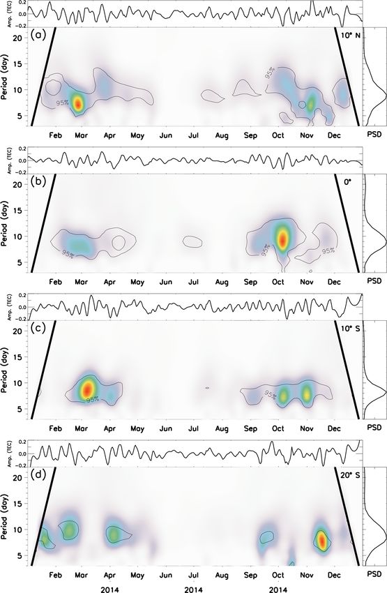
152                                                                A. R. Paulino et al.: Variability of the lunar tidal amplitudes

most important (e.g., Smith and Perlwitz, 2015, and refer-            ual was determined by dividing the residual variation of TEC
ences therein). However, in the last decades, a large num-            by the TEC average.
ber of studies have shown evidence of oscillations with peri-           In the relative residual data, a least-square analysis in a
ods compatible with planetary waves in the thermosphere–              window of 29 d was applied using the following equation:
ionosphere (e.g., Forbes, 1996; Pancheva and Laštovička,
1998; Pancheva et al., 2002; Laštovička, 2006; Abdu et al.,                    3
                                                                                X
2006, 2015; Jonah et al., 2015; Gan et al., 2015; Mo and              y(τ ) =         An cos (nτ + φn ) ,                         (1)
                                                                                n=1
Zhang, 2020, and references therein). The understanding of
how planetary waves can penetrate into the thermosphere–              where τ is the lunar time given by τ = t − ν, and ν is the
ionosphere system has been raised as one of the most im-              age of the Moon, which is set to be 0 at the new Moon. The
portant topics of research in the coupling of the atmospheric         solar time is represented by t, and the amplitudes and phases
layers. Recent studies have given some insights into this topic       of the lunar tide components are represented by An and φn ,
(e.g., Forbes et al., 2014; Gasperini et al., 2017), but further      respectively.
observations and investigations are necessary in order to un-
derstand this coupling.                                               2.2   Filtering
   The lunar semidiurnal tide with period of ∼ 12.424 solar
hours is the most important Moon oscillation for the atmo-            A further description of the methodology to calculate the
sphere in terms of amplitudes. Although the generation of             TEC maps over Brazil was provided by Takahashi et al.
the lunar semidiurnal tides comes from the lower levels of the        (2016). TEC maps have also been used to calculate the am-
atmosphere due to the Moon’s gravitational attraction and in-         plitude and phases of the lunar semidiurnal tide from 2011 to
teraction with vertical motion of the oceans and solid Earth,         2014 over Brazil (Paulino et al., 2017). In the present study,
the lunar tide can propagate to the thermosphere with less in-        the variability due to low and high frequencies in the lunar
fluence by the dissipative process. As the source of the lunar        semidiurnal tide amplitudes observed in those TEC maps is
tide is well known, variations associated with the sources are        investigated in detail.
predictable. Then, the lunar tide can be used as an important            Figure 1 shows the filtering process in the amplitudes of
trace to observe changes in the atmosphere as it propagates           the lunar semidiurnal tide calculated at 10◦ S (magnetic).
vertically. Furthermore, modulation of the lunar semidiurnal             Figure 1a shows the raw amplitudes in TEC units from
tidal amplitudes by planetary waves can be used to explain            2011 to 2014. One can see that there are low- and high-
the presence of these waves in the thermosphere–ionosphere            frequency oscillations in the amplitudes retrieved from the
system, which is the main purpose of the present work. Addi-          TEC. Figure 1b shows the filtered amplitudes considering pe-
tionally, variability of a long period in the lunar semidiurnal       riods greater than 30 d, and Fig. 1c shows the high frequen-
tidal amplitudes is also investigated.                                cies greater than 1/30 d−1 . This filtering process was done
   Data from a network of Global Navigation Satellite Sys-            using a Butterworth kernel low-pass filter of order 1. Mathe-
tem (GNSS) receivers over Brazil were used to calculate the           matically this filter can be written as:
amplitudes and phases of the lunar semidiurnal tide in the
total electron content (TEC) of the ionosphere from 2011 to                             1
                                                                      filter = r                 2n ,                            (2)
2014 (Paulino et al., 2017). In the present work, the tempo-

ral variability of the lunar semidiurnal tidal amplitudes was                      1−       c
extensively investigated showing long- (> 60 d) and short-
period (< 25 d) oscillations.                                         where  is the frequency, c is the cutoff frequency and n is
                                                                      the order (Roberts and Roberts, 1978). This filter is applied
                                                                      to the signal in the domain of the frequency, and then the
2     Analysis and results                                            filtered signal is recovered to the domain of time.
                                                                          Another important point to be analyzed is the possible in-
2.1    Determination of the lunar tide in TEC maps                    fluence of the semidiurnal solar tide in the present results
                                                                      since this oscillation is very close to the semidiurnal lunar
The determination of the lunar semidiurnal tides in TEC               tide. TEC data collected from February to April 2014 at
maps was done according to the Pedatella and Forbes (2010)            30◦ S, 54◦ W were used to validate the present analysis. Fig-
methodology, and only quiet days were considered (Kp < 3)             ure 2 shows the original TEC (panel a), amplitudes of the
in the analysis. After eliminating the geomagnetic influences,        semidiurnal solar tide (panel b), Lomb–Scargle periodogram
a Fourier analysis was performed to extract the subharmonics          for the amplitudes of the solar tide (panel c), amplitudes of
of the solar day (diurnal, semidiurnal and terdiurnal oscilla-        the semidiurnal lunar tide (panel d) and Lomb–Scargle peri-
tions). Effects of the solar rotation were removed using a 27 d       odogram for the amplitudes of the lunar tide. This time inter-
window moving it forward 1 d at time to calculate the mean            val was chosen because it presents a strong quasi 8 d oscilla-
solar day centered in the window. In addition, relative resid-        tion in the amplitudes of the semidiurnal lunar tide, which is

Ann. Geophys., 39, 151–164, 2021                                                            https://doi.org/10.5194/angeo-39-151-2021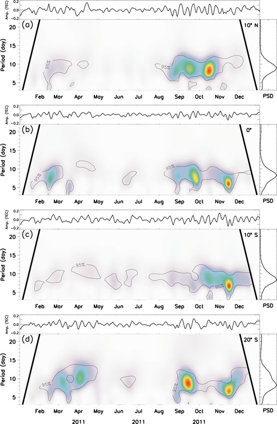
A. R. Paulino et al.: Variability of the lunar tidal amplitudes                                                                      153

Figure 1. (a) Amplitudes of the lunar semidiurnal tide from 2011 to 2014 calculated at 10◦ S (magnetic latitude). (b) Low frequencies
(< 1/30 d−1 ) calculated using a Butterworth kernel filter from amplitudes of (a). (c) Same as (b) but for high frequencies (> 1/30 d−1 ).

going to be discussed later in the text. Furthermore, these ge-        plitudes from 2011 to 2014 for the magnetic latitudes 10◦ N,
ographic coordinates correspond to one of the most southern            0◦ and 10◦ S and 20◦ S.
points of Brazil, where, in general, the solar semidiurnal tide            Figure 3a shows the strong power spectral density (PSD)
is strong compared to the equatorial latitudes.                        associated with the annual and semiannual variations. One
   Figure 2a shows an oscillation roughly around 8 d in the            can also observe that there is a third peak around 120 d, i.e.,
whole data, besides the well pronounced diurnal (24 h) and             a triannual variation. Similar patterns to what are observed at
semidiurnal (12 h) oscillations. Figure 2b shows that there is         10◦ N can be observed at 10◦ S (Fig. 3c) and 20◦ S (Fig. 3d)
no significant oscillation of around 8 d in the amplitude of           as well. At 0◦ (Fig. 3b), annual and semiannual variations
the solar semidiurnal tide, and this is confirmed in Fig. 2c.          were strong; additionally, the triannual variation was weak
Additionally, Fig. 2d shows that the amplitude of the semid-           compared to the other latitudes. Comparing 10◦ N to 10◦ S,
iurnal lunar tide has a well-defined quasi-8 d oscillation, in         it is clear that there are more significant peaks of oscillation
which the confidence level in Fig. 2e appears. These results           in the south, indicating that the long oscillations are not sym-
are very relevant and show that there is no leakage from the           metrical with respect to the magnetic equator.
semidiurnal solar tide in the present results, and the proposed            In order to investigate when the periodicities shown in
methodology satisfactorily separates the solar and lunar com-          Fig. 3 appear more frequently in the dataset, a wavelet anal-
ponents.                                                               ysis was performed, and the results are shown in Fig. 4 with
                                                                       the respective magnetic latitudes. These wavelet charts were
                                                                       calculated based on the methodology of Torrence and Compo
2.3   Long-period oscillations                                         (1998).
                                                                           Figure 4 shows that the annual variation is always present
                                                                       in the amplitude of the lunar tide. Figure 4a shows that the
Considering the filtered amplitudes for periods longer than
                                                                       semiannual variation was present in the two first years, and
30 d, a spectral analysis was performed, and the results are
                                                                       the triannual variation appears more pronounced in the be-
shown in Fig. 3. The Lomb–Scargle periodograms (Lomb,
                                                                       ginning of 2013, which can be composed of oscillations from
1976; Scargle, 1982) were calculated using the filtered am-

https://doi.org/10.5194/angeo-39-151-2021                                                         Ann. Geophys., 39, 151–164, 2021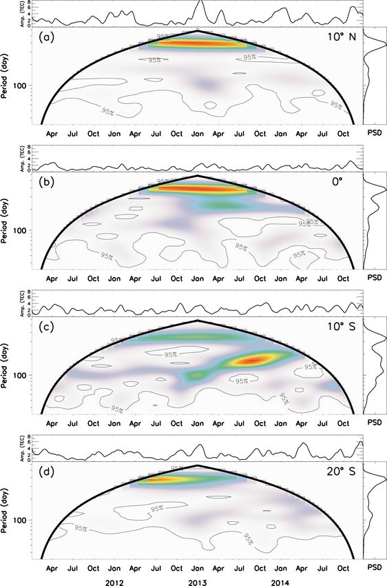
154                                                                    A. R. Paulino et al.: Variability of the lunar tidal amplitudes

                                                                          Figure 3. Lomb–Scargle periodogram for (a) 10◦ N, (b) 0◦ ,
                                                                          (c) 10◦ S and (d) 20◦ S. The horizontal dashed lines represent the
                                                                          confidence level of 99 %, i.e., false alarm probability of 0.01.

                                                                          80 to 120 d. In the beginning of 2014, the triannual variation
                                                                          appeared as well.
                                                                             Figure 4b (magnetic equator) shows that the semiannual
                                                                          variations were strong in the end of 2012 and beginning of
                                                                          2013 with spreading out of this peak to over 200 d. Figure 3b
                                                                          also shows this behavior in the Lomb–Scargle chart. One can
                                                                          also observe short oscillations of 70–80 d in the beginning of
                                                                          2013 and 2014.
                                                                             Figure 4c shows that the semiannual oscillation in the am-
                                                                          plitude of the lunar tide becomes stronger than the annual os-
                                                                          cillation in the second half of 2013. It is important to observe
                                                                          that the triannual oscillation was present in the amplitude of
                                                                          the lunar tide from 2011 to March 2013 and became very
                                                                          strong at the end of this time range, compared to the other
                                                                          latitudes and times. Figure 4c also shows oscillations with
                                                                          periods shorter than 100 d along the whole observed time.
                                                                             Figure 4d shows that the triannual oscillation appeared in
                                                                          2013 and 2014, and at this magnetic latitude, the semiannual
                                                                          oscillation was weaker than the triannual. Oscillations of 70–
                                                                          80 d have the same occurrence observed at 10◦ N.

                                                                          2.4   Short-period oscillations

                                                                          The short-period oscillations observed in the amplitudes of
Figure 2. (a) TEC collected at 30◦ S and 54◦ W from February to           the lunar tide were also investigated in this work. These
April 2014. (b) Amplitudes of the semidiurnal solar tide calculated       oscillations are important, because they can be associ-
from (a). (c) Periodogram for the amplitudes of the semidiurnal           ated with planetary waves revealing relevant aspects in the
solar tide. (d) Amplitudes of the semidiurnal lunar tide calculated       atmosphere–ionosphere coupling from below.
from (a). (e) Periodogram for the amplitudes of the semidiurnal lu-
                                                                             Figure 5 shows the Lomb–Scargle periodogram for the
nar tide. The horizontal dashed line represents the confidence level
                                                                          same latitudes used in Fig. 3 but considering only periods
of 99 %.
                                                                          shorter than 25 d. These periodograms were calculated using
                                                                          the high frequencies in the amplitudes of the lunar semidi-
                                                                          urnal tide as exemplified in Fig. 1c. Figure 5a to d, which

Ann. Geophys., 39, 151–164, 2021                                                           https://doi.org/10.5194/angeo-39-151-2021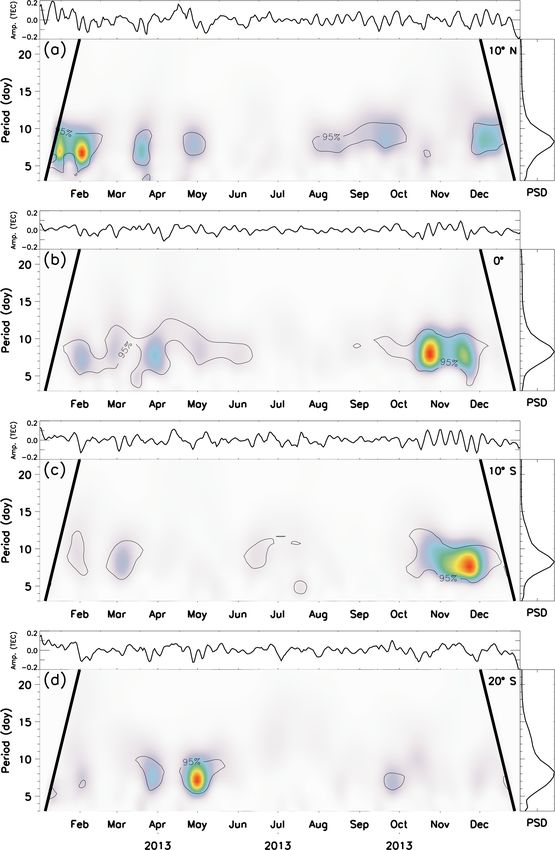
A. R. Paulino et al.: Variability of the lunar tidal amplitudes 155
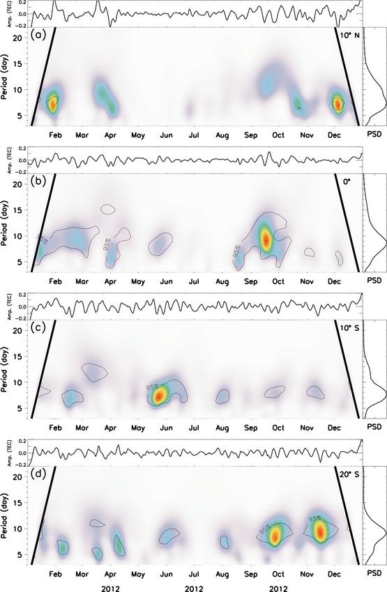
Figure 4. Wavelet analysis for (a) 10◦ N, (b) 0◦ , (c) 10◦ S and (d) 20◦ S. The heavy black lines in the contours represent the cone of influence.
The light black lines show confidence levels of 95 %.
represent the magnetic latitudes from 10◦ N to 20◦ S, shows observed above the significance levels, but they were more
significant periodicities of 7–12 d from 2011 to 2014. Here- sporadic than the Q8D oscillation as will be shown later.
after, we are going to refer to these oscillations as quasi-8 d In order to further investigate the temporal evolution of the
(Q8D) oscillations, although sometimes they can be either short-period oscillation in the amplitudes of the lunar semid-
shorter or longer than 8 d. Similar assumption were used by iurnal tide, wavelet analysis was performed for each year of
Ahlquist (1982). Please note that other long periods were also observations, and the results are shown in Figs. 6, 7, 8 and 9.
One can observe that Q8D is the dominant oscillation along
https://doi.org/10.5194/angeo-39-151-2021 Ann. Geophys., 39, 151–164, 2021156 A. R. Paulino et al.: Variability of the lunar tidal amplitudes
3 Discussion and summary
It is well known that the lunar semidiurnal tide has a pre-
dictable source. Thus, short and long variations observed in
the amplitudes must reveal changes in the atmosphere where
this tidal component is propagating. For instance, annual and
semiannual variations in the amplitudes of the lunar tide have
also been observed in the mesosphere and lower thermo-
sphere (MLT) neutral wind (Paulino et al., 2015). Triannual
variations have been observed and simulated in some atmo-
spheric fields as well (e.g., Pedatella et al., 2012; Pedatella,
2014). However, more investigation is necessary to better un-
derstand the reason for that variability.
The results from Figs. 3 and 4 show that the annual vari-
ation is always present in the amplitudes of the lunar semid-
iurnal tide in the TEC. At the magnetic equator, the PSD of
the annual variation is comparable to the semiannual varia-
Figure 5. Same as Fig. 2 but considering only periods shorter than tion, for instance. However, far from the equator, the annual
25 d. Note that at 0◦ , all periodicities were below the confidence variation is stronger. Furthermore, it seems that the annual
level since the amplitudes were smaller compared to the other lati- variation is out of phase at this latitude compared to the an-
tudes. nual variation observed in MLT winds (Fig. 3, bottom row
of Paulino et al., 2015); i.e., the annual variation maximizes
around January for all latitudes in the TEC, and it maximizes
the whole period of observation. Some particularities are also
around November in the MLT winds. This reinforces the idea
observed in each year, mainly regarding the epoch of the year
that the lunar tide obeys the changes in the atmosphere, and
in which the Q8D wave is stronger.
the observed variability is not due to changes in the sources.
Figure 6 shows the wavelet results for the amplitudes of
Although the semiannual oscillation arose as the second
the lunar semidiurnal tide in 2011. The Q8D oscillation was
peak in the Lomb–Scargle periodogram (Fig. 3) from 2011
stronger from September to November in almost all latitudes.
to 2014, it appeared sporadically and with more intensity
There was a secondary peak of this oscillation from mid-
in lower latitudes. In contrast, the TEC observed in Brazil
February up to April, except at 10◦ S.
shows a semiannual variation and has maxima around the
Figure 7 shows the results for 2012. Again the Q8D os-
equinox during both low and high solar activities (Jonah
cillation was the most important oscillation, but it appeared
et al., 2015).
more frequently through the year, especially out of the mag-
The triannual variation with a period of around 120 d, on
netic equator. One different aspect was that the Q8D oscilla-
average, was the third peak found in the amplitudes of the
tion was strong in February at 10◦ N and in May at 10◦ S.
semidiurnal tide. It was sporadic at 10◦ N; 0◦ ; and 20◦ S. At
In 2013 (Fig. 8), the strength of the Q8D oscillation was
10◦ S, it was present in almost the whole period of observa-
more concentrated in a few months. At 10◦ N, the Q8D os-
tion and it was stronger than the semiannual oscillation dur-
cillation had a larger power spectral density in January and
ing the first two years of observations, except at 20◦ S. Os-
February. At 0 and 10◦ S, the oscillation appeared with more
cillations with 70–80 d period were also observed in all lati-
intensity from late October to December. At 20◦ S, there
tudes sporadically, mainly in the beginning of 2013 and 2014.
were two peaks of the Q8D oscillation in April and May.
In Paulino et al. (2017), it is possible to see that the trian-
Figure 9 shows the power spectral density contour for
nual oscillation appears evident at magnetic latitudes out of
2014. One can observe a regular behavior of the Q8D os-
the equator. It is probable that the combination of the annual
cillation with two peaks around the equinox months.
variation with maximum in the austral summer months and
An important result revealed from the observations is that
semidiurnal variation with maximums around the equinoxes
the Q8D oscillation is always present in the equinox months.
(matching with the TEC maximums) is producing the trian-
From September to November in almost all latitudes and
nual variation in the amplitudes of the lunar semidiurnal tide.
years it was the dominant oscillation. One can also observe
Figure 1a shows roughly a short-period oscillation in the
that the Q8D oscillation appears strong during the winter in
amplitudes of the lunar tide which can be observed in all
2012 and 2013 for some magnetic latitudes.
studied latitudes over Brazil. Sometimes, this short-period
oscillation is stronger and sometimes it is very tenuous. This
behavior is quite interesting, because it was also observed
before (see Fig. 3 of Paulino et al., 2017).
Ann. Geophys., 39, 151–164, 2021 https://doi.org/10.5194/angeo-39-151-2021A. R. Paulino et al.: Variability of the lunar tidal amplitudes 157
Figure 6. Same as Fig. 3 but considering only periods shorter than 25 d during 2011.
An interesting aspect reveled in this work was the peri- Fast Kelvin waves have been observed with periods of typ-
odicity close to 8 d. Based on the literature, there are two ically 6–10 d. It is a kind of wave trapped in the equatorial re-
kinds of large-scale waves with periods close to 8 d: (1) fast gion which has characteristics of gravity waves; i.e., it obeys
Kelvin waves (e.g., Abdu et al., 2015, and references therein) the dispersion relation of gravity waves. Fast Kelvin waves
and (2) quasi-10 d planetary waves (e.g., Forbes and Zhang, are typically observed with large amplitude in the zonal wind
2015; Yamazaki and Matthias, 2019). component and insignificant amplitudes in the meridional
one. As the present Q8D oscillation was observed close to
https://doi.org/10.5194/angeo-39-151-2021 Ann. Geophys., 39, 151–164, 2021158 A. R. Paulino et al.: Variability of the lunar tidal amplitudes Figure 7. Same as Fig. 5 but for 2012. the equator as well as at 20◦ magnetic latitude, which can be and in the MLT winds and associated that oscillation to Fast out of the tropics in the western part of Brazil, this modu- Kelvin waves. Abdu et al. (2015) also observed a Q8D os- lation can have a contribution of other oscillations as well. cillation in the vertical drift of the F region which modulated Some observations have shown that the amplitudes of the the spread-F development. Fast Kelvin wave dominate in altitudes below 90 km (e.g., Figure 10 shows the zonal (solid line) and meridional Lieberman and Riggin, 1997). Dhanya et al. (2012) found (dashed line) thermospheric mean wind at 00:00 UT mea- periodicities close to 8 d in the equatorial electrojet current sured by two Fabry–Pérot interferometers deployed at Ca- Ann. Geophys., 39, 151–164, 2021 https://doi.org/10.5194/angeo-39-151-2021
A. R. Paulino et al.: Variability of the lunar tidal amplitudes                                                             159

Figure 8. Same as Fig. 5 but for 2013.

jazeiras (6.9◦ S, 38.5◦ W) and São João Cariri (7.4◦ S,              Figure 11 shows the Lomb–Scargle periodogram for those
36.5◦ W) during November 2013. Further details about the          data. A strong oscillation of ∼ 6 d can be observed, and it is
operations of those instruments can be found in Makela et al.     likely associated with the presence of fast Kelvin waves in
(2009). One can observe that there is an almost in-phase os-      the equatorial zone. One can also observe a peak of around
cillation of about 1 week in the wind field, possibly suggest-    10 d in both components; however, it was below the confi-
ing the same origin as the observed Q8D oscillation in the        dence level.
amplitude of the lunar tide during this epoch.

https://doi.org/10.5194/angeo-39-151-2021                                                  Ann. Geophys., 39, 151–164, 2021
160                                                               A. R. Paulino et al.: Variability of the lunar tidal amplitudes

Figure 9. Same as Fig. 5 but for 2014.

   In the past years, interest in studying the quasi-10 d wave       ation and spatial (latitude × longitude × altitude) dependen-
(Q10DW) has recovered, primarily due to its association with         cies (Forbes and Zhang, 2015; John and Kumar, 2016).
polar sudden stratospheric warmings (SSWs) (Yamazaki and                Although the present results concentrate on the oscilla-
Matthias, 2019; Mo and Zhang, 2020). Another motiva-                 tions around 8 d in the amplitudes of the semidiurnal lunar
tion was the long-term observation from satellites that al-          tide, these oscillations have some characteristics that are sim-
lows researchers to investigate seasonality, year-to-year vari-      ilar to the Q10DWs as pointed out by Forbes and Zhang
                                                                     (2015). For instance, in some years, they have large ampli-

Ann. Geophys., 39, 151–164, 2021                                                     https://doi.org/10.5194/angeo-39-151-2021
A. R. Paulino et al.: Variability of the lunar tidal amplitudes 161 Figure 10. Zonal (solid line) and meridional (dashed line) mean Figure 12. Zonal (solid line) and meridional (dashed line) wind wind components measured by two Fabry-Pérot interferometers components at 93 km height over Cachoeira Paulista, measured at over Cajazeiras and São João do Cariri, measured at 00:00 UT dur- 02:00 UT during November 2013. ing November 2013. Figure 11. Lomb–Scargle periodogram for (a) zonal and (b) merid- Figure 13. Lomb–Scargle periodogram for (a) zonal and (b) merid- ional wind during November 2013 in the thermosphere over the ional wind during November 2013 at 93 km altitude over Cachoeira equatorial region. Horizontal dotted line represents a significance Paulista. Horizontal dotted line represents a significance level of level of 95 %, i.e., false alarm probability of 0.05. 95 %, i.e., false alarm probability of 0.05. tudes during the equinox and winter months in both hemi- region. Jonah et al. (2015) also observed 8–10 d oscillations spheres. in TEC over Brazil, primarily around the equinoxes. More Observation of waves or oscillations with periods of recently, comprehensive studies on Q10DWs using satellite 8–10 d has been made in the thermosphere–ionosphere. data presented some important temporal and spatial char- For example, Forbes (1996) found Q10DW oscillations in acteristics of these waves below 110 km altitude (Forbes the mesopause and lower thermosphere region using data and Zhang, 2015; John and Kumar, 2016). Additionally, Ya- from medium-frequency (MF) radar and a magnetometer. mazaki and Matthias (2019) and Mo and Zhang (2020) pre- Pancheva and Laštovička (1998) observed fluctuations of sented results associating the Q10Ws to sudden stratospheric 7–8 d from November to December 1994 during an inter- warming events. national campaign. Abdu et al. (2006) studied variation in It is important to note that the observations above showed the equatorial electrojet (EEJ) current and in the MLT wind periods varying from 8 to 10 d in both the mesosphere and and showed the presence of an 8–12 d oscillation around the thermosphere–ionosphere. Forbes and Zhang (2015) showed equinox of 1999 in the equatorial region. Jacobi et al. (2007) slight variation (0.4 d) in the period of Q10W (9.7 to 9.9 d) observed 7–12 d waves in the TEC maps over the European and concluded that the Doppler shift produced by the hori- https://doi.org/10.5194/angeo-39-151-2021 Ann. Geophys., 39, 151–164, 2021
162                                                                 A. R. Paulino et al.: Variability of the lunar tidal amplitudes

zontal wind can change the period of the wave. The present             i.e., the Q8D oscillation, it is clear that there is a discrep-
study uses amplitudes of the lunar semidiurnal tide in lunar           ancy between the observed Q8D oscillation and other os-
time; i.e., the lunar day is about 0.036 d longer than solar day.      cillations observed in the wind. Additionally, according to
Assuming that the observed oscillation has a period of 8.5 d           the theory of planetary waves, the dissipative process into
in lunar time, it corresponds to 8.806 d in solar time. How-           the thermosphere does not allow for direct propagation of
ever, this is not enough to explain the discrepancy between            these wave into high levels. Then, an explanation for obser-
the observed period of the Q10DW in the lower atmosphere               vation of planetary waves in the thermosphere–ionosphere
and the present results.                                               has been suggested, which is basically based on two possi-
   Figure 12 shows the horizontal wind at 93 km altitude               bilities: (1) modulation of the tidal amplitudes, especially the
over Cachoeira Paulista (22.7◦ S, 45.0◦ W) during Novem-               semidiurnal components which can propagate to higher al-
ber 2013 measured at 02:00 UT (universal time). Further de-            titudes into the thermosphere, and/or (2) through the theory
tails about the wind measurements using meteor radar have              of dynamo on the electrodynamics of the ionosphere. The
been published elsewhere (e.g., Paulino et al., 2012). The             present results suggest that maybe a combination of these
temporal evolution of the winds shows some periodic oscil-             two possibilities would be necessary to explain the observed
lations.                                                               modulation in the amplitude of the lunar semidiurnal tide.
   Figure 13 shows the Lomb–Scargle periodogram of the                 However, further investigations are necessary to understand
wind including all temporal measurements at 93 km. A quasi-            this coupling mechanism.
10 d oscillation is shown in both zonal and meridional com-
ponents of the horizontal wind. In the zonal component the
peak of the oscillation was concentrated at 9.7 d, while in the        Data availability. The TEC maps used in this work
meridional one the peak was at ∼ 9 d. The presence of this             are available online on the EMBRACE website (http:
simultaneous oscillation in the MLT wind strongly suggests             //www2.inpe.br/climaespacial, last access: 10 February 2021).
that the observed oscillation in amplitude of the lunar tide           Meteor winds can be requested from Lourivaldo Mota Lima
                                                                       (lourivaldo_mota@yahoo.com.br). Thermospheric winds for São
during November 2013 could have a contribution of this os-
                                                                       João do Cariri and Cajazeiras can be downloaded from the CEDAR
cillation, at least, out of the equator. But the coupling mech-        Madrigal Database (http://cedar.openmadrigal.org, last access:
anism needs further investigations.                                    10 February 2021).
   The main results of this investigation can be summarized
as follows:
  – There is a strong temporal variability in the amplitudes           Author contributions. ARP wrote the article and performed the
    of the lunar semidiurnal tides calculated in the TEC               analysis in the database. FdSA worked on the Lomb–Scargle pe-
    maps over Brazil from 2011 to 2014.                                riodograms. IP revised the article and helped with some analysis
                                                                       of the data. CMW provided the TEC maps. LML provided the me-
  – Annual variation in the lunar semidiurnal tide is always           teor winds. PPB is responsible for the meteor winds and revised the
    present in all observed latitudes, and it is dominant in           article. ISB also revised the article.
    lower latitudes.
  – Semiannual and triannual (∼ 120 d) oscillations were,              Competing interests. The authors declare that they have no conflict
    respectively, the second and third most important long-            of interest.
    period oscillations observed in the amplitudes of the lu-
    nar tide. However, it was observed that there is temporal
    and spatial variability in these oscillations, which allow         Acknowledgements. Ana Roberta Paulino thanks Coordenação
    them to become dominant in a given time interval and               de Aperfeiçoamento de Pessonal de Nível Superior (CAPES)
    latitude range.                                                    for the scholarship. Ana Roberta Paulino, Igo Paulino, Cris-
                                                                       tiano Max Wrasse and Inez Staciarini Batista thank Conselho Na-
  – The observed dominant short-period oscillations in the             cional de Desenvolvimento Científico e Tecnolóligo (CNPq) for the
    amplitudes of the lunar semidiurnal tide had periods be-           financial support. Ana Roberta Paulino and Igo Paulino thank the
    tween 8–11 d, with maxima around the equinoxes. In                 Fundação de Amparo à Pesquisa do Estado da Paraíba. Wavelet
    some years, such as 2013 and 2014, the peaks occurred              software was provided by Christopher Torrence and Gilbert Compo
    in the winter.                                                     and is available at: http://paos.colorado.edu/research/wavelets/ (last
                                                                       access: 10 February 2021). The authors thank Ricardo A. Buriti,
  – Coincident measurements of the horizontal wind during              Jonathan J. Makela and John W. Meriwether for kindly providing
    November 2013 show the presence of a quasi-10 d os-                the Fabry–Pérot interferometer data.
    cillation in MLT at low latitudes (23◦ S) and quasi-6 d
    oscillation in the equatorial thermosphere.
                                                                       Financial support. This research has been supported by the
   Based on the present main results for the short-period os-
                                                                       Conselho Nacional de Desenvolvimento Científico e Tec-
cillations in the amplitudes of the lunar semidiurnal tide,

Ann. Geophys., 39, 151–164, 2021                                                         https://doi.org/10.5194/angeo-39-151-2021
A. R. Paulino et al.: Variability of the lunar tidal amplitudes 163
nológico (grant nos. 460624/2014-8, 303511/2017-6, 307653/2017- stratosphere to the mesosphere-lower thermosphere, Clim. Dy-
0, 405555/2018-0 and 306844/2019-2), Coordenação de Aper- nam., 47, 3863–3881, https://doi.org/10.1007/s00382-016-3046-
feiçoamento de Pessoal de Nível Superior (Prêmio CAPES de tese 2, 2016.
2014) and Fundação de Amparo à Pesquisa do Estado da Paraíba Jonah, O. F., de Paula, E., Muella, M. T. A. H., Dutra, S.
(PRONEX grant 002/2019). L. G., Kherani, E. A., Negreti, P. M. S., and Otsuka, Y.:
TEC variation during high and low solar activities over
South American sector, J. Atmos. Sol.-Terr. Phy., 135, 22–35,
Review statement. This paper was edited by Ana G. Elias and re- https://doi.org/10.1016/j.jastp.2015.10.005, 2015.
viewed by Federico Gasperini and one anonymous referee. Laštovička, J.: Forcing of the ionosphere by waves
from below, J. Atmos. Sol.-Terr. Phy., 68, 479–497,
https://doi.org/10.1016/j.jastp.2005.01.018, 2006.
Lieberman, R. S. and Riggin, D.: High resolution Doppler im-
References ager observations of Kelvin waves in the equatorial mesosphere
and lower thermosphere, J. Geophys. Res.-Atmos., 102, 26117–
Abdu, M., Ramkumar, T., Batista, I., Brum, C., Takahashi, H., 26130, https://doi.org/10.1029/96JD02902, 1997.
Reinisch, B., and Sobral, J.: Planetary wave signatures in the Lomb, N. R.: Least-squares frequency analysis of un-
equatorial atmosphere-ionosphere system, and mesosphere- E- equally spaced data, Astrophys. Space Sci., 39, 447–462,
and F-region coupling, J. Atmos. Sol.-Terr. Phy., 68, 509–522, https://doi.org/10.1007/BF00648343, 1976.
https://doi.org/10.1016/j.jastp.2005.03.019, 2006. Makela, J. J., Meriwether, J. W., Lima, J. P., Miller, E. S.,
Abdu, M. A., Brum, C. G., Batista, P. P., Gurubaran, S., Pancheva, and Armstrong, S. J.: The Remote Equatorial Nighttime Ob-
D., Bageston, J. V., Batista, I. S., and Takahashi, H.: Fast and ul- servatory of Ionospheric Regions Project and the Interna-
trafast Kelvin wave modulations of the equatorial evening F re- tional Heliospherical Year, Earth Moon Planets, 104, 211–226,
gion vertical drift and spread F development, Earth Planet. Space, https://doi.org/10.1007/s11038-008-9289-0, 2009.
67, 1, https://doi.org/10.1186/s40623-014-0143-5, 2015. Mo, X. and Zhang, D.: Quasi-10 d wave modulation of an equa-
Ahlquist, J. E.: Normal-Mode Global Rossby torial ionization anomaly during the Southern Hemisphere
Waves: Theory and Observations, J. Atmos. stratospheric warming of 2002, Ann. Geophys., 38, 9–16,
Sci., 39, 193–202, https://doi.org/10.1175/1520- https://doi.org/10.5194/angeo-38-9-2020, 2020.
0469(1982)0392.0.CO;2, 1982. Pancheva, D. and Laštovička, J.: Planetary wave activity in
Chen, Y.-W. and Miyahara, S.: Analysis of fast and ultrafast Kelvin the lower ionosphere during CRISTA I campaign in autumn
waves simulated by the Kyushu-GCM, J. Atmos. Sol.-Terr. Phy., 1994 (October-−November), Ann. Geophys., 16, 1014–1023,
80, 1–11, https://doi.org/10.1016/j.jastp.2012.02.026, 2012. https://doi.org/10.1007/s00585-998-1014-9, 1998.
Dhanya, R., Gurubaran, S., and Sundararaman, S.: Planetary wave Pancheva, D., Mitchell, N., Clark, R. R., Drobjeva, J., and Las-
coupling of the mesosphere-lower thermosphere-ionosphere tovicka, J.: Variability in the maximum height of the ionospheric
(MLTI) region during deep solar minimum 2005-2008, Indian F2-layer over Millstone Hill (September 1998–March 2000); in-
J. Radio Space, 41, 271–284, 2012. fluence from below and above, Ann. Geophys., 20, 1807–1819,
Forbes, J. M.: Planetary Waves in the Thermosphere- https://doi.org/10.5194/angeo-20-1807-2002, 2002.
Ionosphere System, J. Geomagn. Geoelectr., 48, 91–98, Paulino, A., Batista, P., and Clemesha, R.: Lunar tides in the
https://doi.org/10.5636/jgg.48.91, 1996. mesosphere and lower thermosphere over Cachoeira Paulista
Forbes, J. M. and Zhang, X.: Quasi-10-day wave in the (22.7◦ S; 45.0◦ W), J. Atmos. Sol.-Terr. Phy., 78–79, 31–36,
atmosphere, J. Geophys. Res.-Atmos., 120, 11079–11089, https://doi.org/10.1016/j.jastp.2011.04.018, 2012.
https://doi.org/10.1002/2015JD023327, 2015. Paulino, A. R., Batista, P. P., Lima, L. M., Clemesha, B. R., Buriti,
Forbes, J. M., Zhang, X., and Bruinsma, S. L.: New perspectives R. A., and Schuch, N.: The lunar tides in the mesosphere and
on thermosphere tides: 2. Penetration to the upper thermosphere, lower thermosphere over Brazilian sector, J. Atmos. Sol.-Terr.
Earth Planet. Space, 66, 122, https://doi.org/10.1186/1880-5981- Phy., 133, 129–138, https://doi.org/10.1016/j.jastp.2015.08.011,
66-122, 2014. 2015.
Gan, Q., Yue, J., Chang, L. C., Wang, W. B., Zhang, S. D., and Paulino, A. R., Lima, L. M., Almeida, S. L., Batista, P. P., Batista,
Du, J.: Observations of thermosphere and ionosphere changes I. S., Paulino, I., Takahashi, H., and Wrasse, C. M.: Lunar tides in
due to the dissipative 6.5-day wave in the lower thermosphere, total electron content over Brazil, J. Geophys. Res.-Space, 122,
Ann. Geophys., 33, 913–922, https://doi.org/10.5194/angeo-33- 7519–7529, https://doi.org/10.1002/2017JA024052, 2017.
913-2015, 2015. Pedatella, N. M.: Observations and simulations of the ionospheric
Gasperini, F., Forbes, J. M., and Hagan, M. E.: Wave coupling lunar tide: Seasonal variability, J. Geophys. Res.-Space, 119,
from the lower to the middle thermosphere: Effects of mean 5800–5806, https://doi.org/10.1002/2014JA020189, 2014.
winds and dissipation, J. Geophys. Res.-Space, 122, 7781–7797, Pedatella, N. M. and Forbes, J. M.: Global structure of the lunar
https://doi.org/10.1002/2017JA024317, 2017. tide in ionospheric total electron content, Geophys. Res. Lett.,
Jacobi, C., Jakowski, N., Pogoreltsev, A., Fröhlich, K., Hoffmann, 37, l06103, https://doi.org/10.1029/2010GL042781, 2010.
P., and Borries, C.: The CPW-TEC project: Planetary waves in Pedatella, N. M., Liu, H.-L., and Richmond, A. D.: Atmospheric
the middle atmosphere and ionosphere, Adv. Radio Sci., 5, 393– semidiurnal lunar tide climatology simulated by the Whole At-
397, https://doi.org/10.5194/ars-5-393-2007, 2007. mosphere Community Climate Model, J. Geophys. Res.-Space,
John, S. R. and Kumar, K. K.: Global normal mode planetary wave 117, a06327, https://doi.org/10.1029/2012JA017792, 2012.
activity: a study using TIMED/SABER observations from the
https://doi.org/10.5194/angeo-39-151-2021 Ann. Geophys., 39, 151–164, 2021164 A. R. Paulino et al.: Variability of the lunar tidal amplitudes Roberts, J. and Roberts, T. D.: Use of the Butterworth low-pass fil- Torrence, C. and Compo, G. P.: A Practical ter for oceanographic data, J. Geophys. Res.-Oceans, 83, 5510– Guide to Wavelet Analysis, B. Am. Meteo- 5514, https://doi.org/10.1029/JC083iC11p05510, 1978. rol. Soc., 79, 61–78, https://doi.org/10.1175/1520- Scargle, J. D.: Studies in astronomical time series analysis. II. Sta- 0477(1998)0792.0.CO;2, 1998. tistical aspects of spectral analysis of unevenly spaced data, As- Yamazaki, Y. and Matthias, V.: Large-Amplitude Quasi- trophys. J., 263, 835–853, https://doi.org/10.1086/160554, 1982. 10-Day Waves in the Middle Atmosphere During Final Smith, A. K. and Perlwitz, J.: Middle Atmosphere|Planetary Warmings, J. Geophys. Res.-Atmos., 124, 9874–9892, Waves, pp. 1–11, Academic Press, Oxford, https://doi.org/10.1029/2019JD030634, 2019. https://doi.org/10.1016/B978-0-12-382225-3.00229-2, 2015. Takahashi, H., Wrasse, C. M., Denardini, C. M., Pádua, M. B., de Paula, E. R., Costa, S. M. A., Otsuka, Y., Shiokawa, K., Monico, J. F. G., Ivo, A., and Sant’Anna, N.: Ionospheric TEC Weather Map Over South America, Adv. Space Res., 14, 937– 949, https://doi.org/10.1002/2016SW001474, 2016. Ann. Geophys., 39, 151–164, 2021 https://doi.org/10.5194/angeo-39-151-2021
You can also read