Comparisons of Real-World Vehicle Energy Efficiency with Dynamometer-Based Ratings and Simulation Models - MDPI
←
→
Page content transcription
If your browser does not render page correctly, please read the page content below

Article

Comparisons of Real-World Vehicle Energy Efficiency with
Dynamometer-Based Ratings and Simulation Models
Karim Hamza 1,*, Kang-Ching Chu 1, Matthew Favetti 2, Peter Keene Benoliel 2, Vaishnavi Karanam 2,
Kenneth P. Laberteaux 1 and Gil Tal 2

                                          1 Toyota Motor North America R&D; Ann Arbor, MI 48105, USA; jean.chu@toyota.com (K.-C.C.);
                                            ken.laberteaux@toyota.com (K.P.L.)
                                          2 Institute of Transportation Studies, University of California at Davis, Davis, CA 95616, USA;

                                            mpfavetti@ucdavis.edu (M.F.); pkbenoliel@ucdavis.edu (P.K.B.); vckaranam@ucdavis.edu (V.K.);
                                            gtal@ucdavis.edu (G.T.)
                                          * Correspondence: karim.hamza@toyota.com; Tel.: +1-734-546-2423

                                          Abstract: Software tools for fuel economy simulations play an important role during design stages
                                          of advanced powertrains. However, calibration of vehicle models versus real-world driving data
                                          faces challenges owing to inherent variations in vehicle energy efficiency across different driving
                                          conditions and different vehicle owners. This work utilizes datasets of vehicles equipped with
                                          OBD/GPS loggers to validate and calibrate FASTSim (software originally developed by NREL) ve-
                                          hicle models. The results show that window-sticker ratings (derived from dynamometer tests) can
                                          be reasonably accurate when averaged across many trips by different vehicle owners, but success-
                                          fully calibrated FASTSim models can have better fidelity. The results in this paper are shown for
Citation: Hamza, K.; Chu, K.-C.;
                                          nine vehicle models, including the following: three battery-electric vehicles (BEVs), four plug-in
Favetti, M.; Benoliel, P.K.; Karanam,
V.; Laberteaux, K.P.; Tal, G.
                                          hybrid electric vehicles (PHEVs), one hybrid electric vehicle (HEV), and one conventional internal
Comparisons of Real-World Vehicle         combustion engine (CICE) vehicle. The calibrated vehicle models are able to successfully predict
Energy Efficiency with                    the average trip energy intensity within ±3% for an aggregate of trips across multiple vehicle own-
Dynamometer-Based Ratings and             ers, as opposed to within ±10% via window-sticker ratings or baseline FASTSim.
Simulation Models. World Electr.
Veh. J. 2021, 12, 161. https://doi.org/   Keywords: electrified powertrains; vehicle modeling and simulation; vehicle energy efficiency
10.3390/wevj12040161

Academic Editor: Joeri Van Mierlo

                                          1. Introduction
Received: 8 August 2021
Accepted: 15 September 2021
                                                Many software tools exist for modeling the fuel economy of vehicles, as surveyed in
Published: 25 September 2021              [1]. Depending on the underlying modeling approach, one may classify the tools into the
                                          following: (i) direct simulation models that are physics-based (termed “White-box” in [1]),
Publisher’s Note: MDPI stays neu-         (ii) empirical models that are primarily data-inference-based (termed “Black-box” in [1]),
tral with regard to jurisdictional        and (iii) hybrid models that combined some traits of both empirical and physics-based
claims in published maps and institu-     models (termed “White-box” in [1]). Examples of physics-based models include Autono-
tional affiliations.                      mie [2] and FASTSim [3], which are endorsed by the U.S. Department of Energy [4]. Ex-
                                          amples of empirical models include MOVES [5], which is developed and maintained by
                                          the U.S. Environmental Protection Agency (EPA) and EMFAC [6], which is utilized by the
                                          California Air Resources Board. Furthermore, categorically speaking, window-sticker rat-
Copyright: © 2021 by the authors. Li-     ings published by the EPA [7] are another form of a (simple) black-box model.
censee MDPI, Basel, Switzerland.                Black-box models have the advantage of being grounded to real-world data, but their
This article is an open access article
                                          shortcomings include (i) the possibility of reduced accuracy when applied to smaller sub-
distributed under the terms and con-
                                          populations of vehicles, (ii) the need for large amounts of data in order to properly cali-
ditions of the Creative Commons At-
                                          brate, and (iii) the difficulty in predicting the performance of vehicle models that do yet
tribution (CC BY) license (http://crea-
                                          not exist in the real-world. White-box models (physics-based) on the other hand can be
tivecommons.org/licenses/by/4.0/).
                                          easily modified to explore new design parameter settings, but validity of the model (i.e.,
                                          whether a new prototype will perform as predicted by the software) remains an important

World Electr. Veh. J. 2021, 12, 161. https://doi.org/10.3390/wevj12040161                                              www.mdpi.com/journal/wevj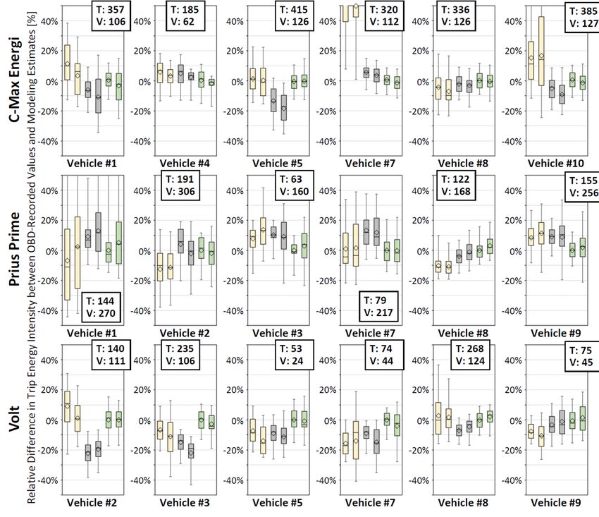
World Electr. Veh. J. 2021, 12, 161                                                                                         2 of 13

                                      issue. As new vehicle designs are of primary interest, the current work focuses on physics-
                                      based models, and more specifically FASTSim [3], owing to it being (relatively) computa-
                                      tionally-light, open-source, and freely accessible to the general public.
                                            While detailed physics-based models such as Autonomie are becoming popular for
                                      future transportation systems simulation, such as autonomous vehicles [8], data-based
                                      approaches also appear to remain popular in recent literature [9,10]. Previous work by the
                                      authors in [11] aimed to strike a balance between the attractive features of a computation-
                                      ally light physics-based model (FASTSim) along with the calibration capability of data-
                                      based approaches. The previous work by the authors in [11] proposed three tunable pa-
                                      rameters that constitute correction terms for passenger and cargo weight, as well as aux-
                                      iliary and traction power. The results of the approach in [11] were shown for three battery-
                                      electric vehicle (BEV) models (Leaf, Bolt, Model S) and three plug-in hybrid electric vehi-
                                      cle (PHEV) models (C-Max Energi, Prius Prime, Volt).
                                            The current paper extends the previous work into an additional minivan PHEV
                                      model (Pacifica Hybrid), a non-plug-in hybrid electric vehicle (HEV) model (Prius HEV),
                                      as well as an SUV conventional internal combustion engine (CICE) vehicle model (CR-V).
                                      The current paper also delves deeper (for all nine considered vehicle models) into exam-
                                      ining how the driving conditions from different vehicle owners of the same vehicle model
                                      can pose challenges to the construction of “useful” calibrated models capable of generali-
                                      zation across multiple owners.
                                            The rest of the paper is organized as follows. Section 2 provides an overview of the
                                      source for real-world vehicles trip data and conducts an analysis that highlights variations
                                      in trip energy intensity (energy per distance travelled), Section 3 provides a summary of
                                      the vehicle models’ calibration approach and results of the optimized values for the tuning
                                      parameters, and Section 4 showcases the performance of the calibrated vehicle simulation
                                      models. The paper then ends with a brief summary of conclusions and future work.

                                      2. Real-World Vehicles Trip Data
                                            Datasets of real-world driving analyzed in this work are but a subset of large-scale
                                      data collection effort by UC-Davis Institute of Transportation Studies, the eVMT Project
                                      [12]. Part of the eVMT project involves OBD/GPS monitoring of all vehicles in survey par-
                                      ticipant households that own a BEV or PHEV. To maintain privacy for survey participants,
                                      only the following second-by-second trip information was utilized within the current
                                      work for simulation of energy/fuel consumption: (i) vehicle speed, (ii) road slope, and (iii)
                                      cabin heating or air-conditioning power. In order to compare/validate simulation models,
                                      OBD record of energy/fuel utilization parameters are also examined, but only totals for
                                      whole trips. Furthermore, for additional privacy consideration, even after removal of sen-
                                      sitive parts of the data, computational analysis involving individual trips is carried out in
                                      a secured environment, with only bulk results presented.
                                            Box-plots for trip energy intensity, defined as vehicle energy usage per distance trav-
                                      elled (with units of kWh/mile or gal/mile), are shown in Figure 1. The analyzed dataset
                                      includes trips from up to 10 (fewer real-world vehicles were available for some models)
                                      different real-world vehicles per vehicle model. For PHEVs, whose trips can include both
                                      electricity and gasoline usage, all gasoline amounts were transformed into equivalent elec-
                                      tric energy (kWh) by multiplying by the fuel heating value and average vehicle efficiency
                                      in charge sustaining mode, thus allowing trip energy intensity of PHEVs to be visualized
                                      via single box-plots (as opposed to splitting electricity and gasoline, which could have
                                      created biases due to differences in driving patterns for trips that involve gasoline usage).
                                      Box-plots provide a convenient and compact way of visualizing data that include statisti-
                                      cal variations. The bottom and top lines of the box correspond to the 25th and 75th per-
                                      centiles, respectively, of the cumulative distribution, while the middle line corresponds to
                                      the median value. The bottom and top extension lines mark the 5th and 95th percentiles,
                                      respectively, while the average value for the distribution is marked by a diamond shape.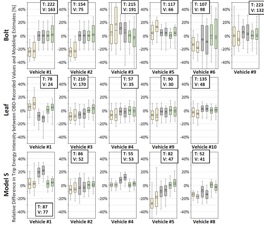
World Electr. Veh. J. 2021, 12, 161                                                                                     3 of 13

                                      Aside from individual vehicle-household box plots, a combined “zone-wide” (darker
                                      tone) box-plot is shown in Figure 1 for all trips by all vehicles of a given model.

                     Figure 1. Baseline estimated costs of CICE and various plug-in vehicle models for 2018 and 2030.
World Electr. Veh. J. 2021, 12, 161                                                                                      4 of 13

                                           Additional data provided in Figure 1 include the number of trips in the data sample
                                      for each vehicle, which is shown between brackets below the vehicle ID on the horizontal
                                      axis, as well as equivalent EPA widow-sticker kWh/mile or gal/mile value for the com-
                                      bined cycle (as obtained from [7]), which is marked via a horizontal dashed line. The sec-
                                      ondary vertical axis in Figure 1 (with red text) showcases the relative difference in trip
                                      energy intensity when referenced to the OBD average value for all trips by all vehicle
                                      samples of a vehicle model.
                                           Keeping in mind that OBD readings can have their own error margin, and that ac-
                                      counting for such errors is beyond the scope of current work, some notable observations
                                      about Figure 1 include the following:
                                      •   For the vast majority of the considered individual vehicle owners, some of their trips
                                          have higher energy intensity than the window-sticker value, while some other trips
                                          have lower energy intensity (other than a few cases such as the Bolt owner #2 and
                                          Model S owner #5, the dashed line in Figure 1 lies between the 5th and 95th percen-
                                          tiles marked by the extension lines of box-plots);
                                      •   Window-sticker values can be reasonably good (within approximately ±10%) at pre-
                                          dicting the average energy intensity across multiple vehicle owners (comparing the
                                          average value for darker tone box plots with the dashed line in Figure 1), but the
                                          average energy intensity for some individual vehicle owners can be off from the win-
                                          dow-sticker value by more than 20%, such as the Model S owner #4 in Figure 1;
                                      •   Individual trips by vehicle owners may occasionally be different than the average
                                          across owners (reading the 5th and/or 95th extension lines on the secondary vertical
                                          axis in Figure 2) by more than 50%. By extent, the window-sticker values can also be
                                          off by more than 50% for some individual trips.
World Electr. Veh. J. 2021, 12, 161         5 of 13

                                      (a)
World Electr. Veh. J. 2021, 12, 161 6 of 13
(b)World Electr. Veh. J. 2021, 12, 161 7 of 13
(c)
Figure 2. (a) Individual vehicle samples (Prius HEV, CR-V, Pacifica Hybrid) validity assessment of trip energy intensity.
(b) Individual vehicle samples (C-Max Energi, Prius Prime, Volt) validity assessment of trip energy intensity. (c) Individ-
ual vehicle samples (Bolt, Leaf, Model S) validity assessment of trip energy intensity.
The main insights from such observations could be summarized as highlighting that
variations in trip energy intensity do exist across different vehicle owners and within dif-
ferent trips by same vehicle owners. Some of those variations (attributed to variations in
trip speed, acceleration aggressiveness, or road slope) may be possible to reproduce in
software simulations, while other sources of variation (such as unknown passenger/cargo
weight or head wind speed) can be very difficult to predict and account for. As such, tun-
ing of software models compared with real-world energy recording is done with a mind-
set of error reduction, but with the understanding that errors cannot be completely elimi-
nated.World Electr. Veh. J. 2021, 12, 161 8 of 13
3. Model Calibration
A calibration approach using three tuning parameters for physics-based simulation
models (applied to FASTSim) was previously introduced by the authors. For details (in-
cluding mathematical derivation), readers are referred to [11]. An overview of the three
parameters is explained as follows:
αT is a scaling factor that adjusts the total traction power at every time instant (calcu-
lated by FASTSim to account for acceleration, wind drag, rotational inertia, road
slope, and tire rolling resistance).
αM is a correction mass (in (kg)) to account for differences across vehicle owners in pas-
senger and cargo weight from the default (136 kg) value in FASTSim.
αA is a constant additional power (in (kW)) that takes the form of a correction term for
auxiliary power, but is intended to also account for other unknown effects.
An estimation of appropriate values for the tuning parameters is conducted via an
optimization procedure that seeks to minimize a weighed error function for differences
between OBD energy records and simulation predictions, for several trips across multiple
vehicle owners. The results of the optimized tuning parameters are summarized in Table
1. As with typical meta-modeling approaches [13], tuning of the models is conducted on
a subset of data (referred to as the set of trips “T”), then verification is conducted on a
different set of trips that were not included in the optimization (referred to as the set of
trips “V”). For that reason, only a subset of vehicles from Figure 1 (ones that have a suffi-
cient number of trips that can be partitioned into sets T and V) are included in Table 1.
Table 1. Annual VMT and UF based on the CHTS dataset.
Tuning Parameter Values
Vehicle Model Vehicle Sample ID αT αM [kg] αA [kW]
1 0.94 173.9 0.071
2 0.94 −14.2 2.084
3 0.94 −50.0 0.009
Bolt 5 0.94 60.3 0.689
6 0.94 205.8 1.108
9 0.94 29.3 0.823
(Group) 0.94 36.9 0.899
1 0.98 243.2 0.839
3 0.98 217.5 0.878
4 0.98 238.8 0.832
Leaf
9 0.98 −5.5 0.741
10 0.98 −8.1 0.382
(Group) 0.98 144.3 0.746
1 0.96 −50.0 0.000
2 0.96 224.1 0.782
4 0.96 198.6 0.308
Model S
5 0.96 167.6 2.765
8 0.96 248.6 1.803
(Group) 0.96 117.4 0.947
1 0.92 154.9 0.655
4 0.92 105.7 0.000
5 0.92 155.5 1.247
C-Max Energi 7 0.92 −50.0 0.000
8 0.92 181.5 1.008
10 0.92 194.5 0.310
(Group) 0.92 118.0 0.486World Electr. Veh. J. 2021, 12, 161 9 of 13
1 0.96 −18.1 0.545
2 0.96 26.1 0.933
3 0.96 69.1 0.053
Prius Prime 7 0.96 −27.6 0.000
8 0.96 106.6 1.177
9 0.96 82.4 0.150
(Group) 0.96 54.7 0.445
2 1.02 155.7 1.024
3 1.02 122.8 1.567
5 1.02 226.8 0.670
Volt 7 1.02 257.8 0.605
8 1.02 73.2 0.364
9 1.02 58.7 0.000
(Group) 1.02 131.6 0.830
1 1.00 218.4 0.216
2 1.00 104.9 0.001
Pacifica Hybrid 3 1.00 221.3 0.954
5 1.00 316.3 1.359
(Group) 1.00 209.3 0.605
1 1.02 −47.3 0.993
2 1.02 −41.2 0.479
Prius HEV
3 1.02 −10.7 0.559
(Group) 1.02 −44.9 0.889
1 1.02 57.6 0.212
2 1.02 159.1 2.295
CR-V
3 1.02 40.3 2.020
(Group) 1.02 71.7 1.445
In the design philosophy of the calibration approach, αT is intended to account for
minor discrepancies in the modelled powertrain components such as engine, motor, and
transmission. As such, in a properly constructed physics-based model, when conducting
optimization in order to estimate values for (αT, αA, αM), the optimized value for αT should
be close to 1 (and its value is considered a sanity-check). Furthermore, only one value for
αT per vehicle model is considered in the optimization, while (αA, αM) are permitted by the
optimization to have different values for each individual vehicle owner. After conducting
the optimization, a final step includes averaging of the parameter values across different
owners in order to provide a more generic “group-wide” estimate, as shown in Table 1.
4. Results and Discussion
One of the key philosophies in the development of FASTSim by its original authors
at NREL was to emphasize reasonable accuracy (within ±10% per [14]) in favor of fast
computations that allow the simulation of large sets of real-world driving. In that sense,
the key advantage of “baseline” FASTSim may not so much be its ability to provide better
predictions than window-sticker ratings (which are also in the same ball-park of ±10%
when examining averages across multiple vehicle owners in Figure 1), but in its ability to
provide predictions about vehicle designs that do not exist in the market yet. For example,
FASTSim could simulate a 150-mile electric range version of C-Max or change the power-
train of a conventional ICE pickup truck model into a 300-mile range BEV. For that reason,
the validity assessment of fuel economy models in this section will examine the statistical
distribution (via box plots) for the relative difference in trip energy intensity (per Equation
(1)) for three predictors:World Electr. Veh. J. 2021, 12, 161 10 of 13
• Window-sticker-based prediction, in which the prediction for every trip is simply the
combined cycle rating from the fuel economy guide [7].
• Baseline FASTSim models, as published by NREL in the 2018 public version of
FASTSim [3]. It should be noted, however, that the public version of FASTSim does
not include all vehicle models considered in the current study (Table 1). Thus, a
“baseline” FASTSim model could not be examined for Pacfica Hybrid, Prius HEV, or
CR-V.
• FASTSim models with tuning, per the adopted calibration approach.
The relative difference in trip energy intensity (λ), whose statistics are used as an
error metric for comparison between fuel economy prediction models, is defined as fol-
lows:
λ jm =
(E m
j − Eoj )
, j ∈{T , V } (1)
Eoj
where E is the equivalent energy intensity (in (kWh/mile) or (gal/mile)) for some trip j,
with the superscript o indicating the OBD-logged value for the trip, while the superscript
m indicates some other model for estimation, with T and V indicating the tuning and val-
idation sets of trips, respectively.
A comparison of trip energy intensity estimation models for each of the individual
vehicle samples (as listed in Table 1) is shown in Figure 2. As trips of each vehicle sample
are split into tuning and verification subsets of trips, the box-plots in Figure 2 are shown
in pairs, with same color tone with the color tone indicating the model that was used for
the estimation of trip energy intensity. In each pair of box-plots, the first (to the left) is for
the tuning set of trips, while the second (to the right) is for the verification set of trips. It
should be noted that window-sticker-based estimates and baseline FASTSim involve no
optimization-based tuning, thus their performance should not differ much between the
tuning and verification sets of trips. However, as the trip sets are different, they are still
reported in separate box-plots in Figure 2.
Notable observations from Figure 2 include the following:
• The average value (diamond marker) for tuned FASTSim models for the tuning set
of trips (left box-plot in the green color tone pairs) remains within ±1% for all vehicle
samples of all considered vehicle models. This is an indication of success for the op-
timization process being able to find a good solution for the tuning parameter values,
but not necessarily an indication that the tuned FASTSim models can generalize well.
• The average value for tuned FASTSim models for the verification set of trips (right
box-plot in the green color tone pairs) is mostly within ±5%, with the exception of
Bolt vehicle #1, CR-V vehicle #2, and Prius Prime vehicle #1, which have errors of
−6.6%, +6.0%, and +5.2%, respectively.
• The average value for window-sticker based estimates (diamond marker in either of
the yellow color tone box-plot pairs) is outside the bounds of ±10% on some vehicle
samples across different vehicle models, with a few cases outside ±15% and one ex-
treme case (C-Max Energi vehicle #7) exceeding 40%.
• The average value for baseline FASTSim (diamond marker in either of the gray color
tone box-plot pairs) is mostly within ±15%, with the exception of Model S vehicle #1,
Volt vehicles #2 and #3, C-Max Energi vehicle #5, which have errors of +22.0%,
−22.3%, −22.0% and −19.4% respectively.
Observations from Figure 2 further highlight the limitation of window-sticker-based
predictions when it comes to individual vehicle owners, which is consistent with the gen-
eral message in the fuel economy guide that individual mileage can vary [7]. Baseline
FASTSim models are mostly at the same level of accuracy as window-sticker-based pre-
dictions, and may have a bit of an advantage in being able to avoid large errors in extreme
case samples (such as C-Max Energi vehicle #7 in Figure 2). Tuned FASTSim models onWorld Electr. Veh. J. 2021, 12, 161 11 of 13
the other hand are observed to exhibit superior prediction performance of trip energy in-
tensity (even on trips that were not part of the model tuning process), and this predictive
capability was observable across all vehicle samples in all considered vehicle models. In-
dividually calibrated vehicle models, however, imply that each vehicle (for each owner)
can have a different value for correction mass and auxiliary power, which poses a chal-
lenge when the goal is to construct vehicle models that generalize across multiple owners.
For vehicle models that are capable of generalizing across different vehicle owners,
we test the “group-wide” estimate for the tuning parameters (αT, αA, αM) in Table 1. The
group-wide estimate for (αT, αA, αM) is essentially a weighted average (by total miles
driven) for the vehicles that have been individually tuned (per Figure 2). The test set of
trips for the group-wide tuned models includes trips in the tuning set, verification set, as
well as trips by vehicles samples in Figure 1 that were not included in the tuning process
at all. The results of the group-wide validity assessment are shown in Figure 3, in which
notable observations include the following:
• The average value (diamond shape) for both window-sticker-based estimates (yellow
color tone box plots in Figure 3) and baseline FASTSim (gray color tone box plots)
remains mostly within ±10% error bounds, with the exception of C-Max Energi, and
CR-V for window-sticker-based estimates, and Volt for baseline FASTSim.
• The average value for tuned FASTSim models (diamond shape of green color tone
box plots in Figure 3) remains within ±3% error for all the studied vehicle models.
The worst observed cases were for Prius Prime and CR-V, at +2.8% and +2.2%, re-
spectively.
Figure 3. Validity assessment for trip energy intensity estimation models for whole groups of vehicle samples.
It ought to be noted that a limitation of the overall calibration approach (where three
tuning parameters adjust the FASTSim model for a group of vehicle owners) is that indi-
vidual usage conditions by some owners or certain trips by some owners may vary sig-
nificantly from the “typical” expectation of the calibrated models. For example, one trip
may involve a heavier than normal load of passengers and cargo (thus not adhering to the
expected value for correction mass parameter) and/or take place during significantly
worse than normal weather conditions. Such unusual trips do show up in Figure 3 when
examining the 5th and 95th percentile trips (extension lines of the box plots), which, evenWorld Electr. Veh. J. 2021, 12, 161 12 of 13
for the calibrated models, can extend up to nearly ±30% error (as observed for models of
the Bolt and Prius Prime in Figure 3).
5. Conclusions
This paper adopted a calibration approach for FASTSim and tested its validity for
nine vehicle models including a variety of powertrains (three BEVs, four PHEVs, one
HEV, and one CICE). The accuracy in predicting the average energy intensity was within
±7% in verification set of trips by individual vehicle owners (compared with more than
±15% for baseline FASTSim and window-sticker-based estimation), and within ±3% when
combining trips across multiple vehicle owners (compared with ±10% for baseline
FASTSim and window-sticker-based estimation). It was thus demonstrated that the pro-
posed calibration approach (with only three tuning parameters), while requiring some
additional optimization work compared with baseline FASTSim, can improve the fidelity
of the vehicle models for representative groups of vehicle owners. Achieving high accu-
racy in the simulation of individual trips, however, remains a challenge owing to various
unforeseeable uncertainties that some trips may have.
It also ought to be noted that the calibration approach is not necessarily specific to
FASTSim, thus future work may include implementation and testing with other physics-
based models for vehicle fuel economy simulations. Future work may also consider com-
parison with other black-box type estimators (besides window-sticker-based estimation),
such as MOVES and EMFAC.
Author Contributions: Conceptualization, methodology K.H.; software, data cleaning, M.F. and
K.H.; formal analysis, K.H.; M.F., P.-K.B., V.K., K.-C.C., K.P.L., and G.T.; writing—original draft
preparation, K.H. and K.C.C.; writing—review and editing, K.C.C., K.P.L., and G.T. All authors
have read and agreed to the published version of the manuscript.
Funding: This research received no external funding.
Data Availability Statement: Due to data handling privacy agreements, restrictions apply to ac-
cessing the eVMT survey dataset utilized in this study. For limited access, please contact the Uni-
versity of California at Davis Institute of Transportation Studies.
Acknowledgments: The authors would like to thank the researchers at NREL whose work contrib-
uted to bringing FASTSim out to the world. Special thanks are also due to Jeff Gonder and Aaron
Brooker at NREL for insightful discussions about the methodology proposed in this work.
Conflicts of Interest: The authors declare no conflict of interest.
References
1. Zhou, M.; Jin, H.; Wang, W. A Review of Vehicle Fuel Consumption Models to Evaluate Eco-Driving and Eco-Routing. Transp.
Res. Part D 2016, 49, 203–218.
2. Argonne National Laboratory. Autonomie: Automotive System Design. Available online: https://www.autonomie.net/ (ac-
cessed on 18 October 2019).
3. National Renewable Energy Laboratory. Future Automotive Systems Technology Simulator. Available online:
http://www.nrel.gov/transportation/fastsim.html (accessed on 18 October 2019).
4. US Department of Energy; Vehicle Technologies Office. Modeling and Simulation. Available online: https://energy.gov/eere/ve-
hicles/vehicle-technologies-office-modeling-and-simulation (accessed on 18 October 2019).
5. US Environmental Protection Agency. MOVES and Other Mobile Source Emissions Models. Available online:
https://www.epa.gov/moves (accessed on 18 October 2019).
6. California Air Resources Board. MSEI - Modeling Tools. Available online: https://ww2.arb.ca.gov/our-work/programs/mobile-
source-emissions-inventory/msei-modeling-tools (accessed on 18 October 2019).
7. US Department of Energy; Environmental Protection Agency. The official U.S. Government source for fuel economy infor-
mation. Available online: https://www.fueleconomy.gov/ (accessed on 18 October 2019).
8. Islam, E.; Moawad, A.; Kim, N.; Rousseau, A. Vehicle Electrification Impacts on Energy Consumption for Different Connected-
Autonomous Vehicle Scenario Runs. World Electr. Veh. J. 2020, 11, 9.
9. Kim, H.; Pyeon, H.; Park, J.; Hwang, J.; Lim, S. Autonomous Vehicle Fuel Economy Optimization with Deep Reinforcement
Learning. Electronics 2020, 9, 1911.World Electr. Veh. J. 2021, 12, 161 13 of 13
10. Luo, Y.; Xiang, D.; Zhang, S.; Liang, W.; Sun, J.; Zhu, L. Evaluation on the Fuel Economy of Automated Vehicles with Data-
Driven Simulation Method. Energy AI 2021, 3, 100051.
11. Hamza, K.; Chu, K.C.; Favetti, M.; Benoliel, P.; Karanam, V.; Laberteaux, K.; Tal, G. Validity Assessment and Calibration Approach
for Simulation Models of Energy Efficiency of Light-Duty Vehicles; SAE World Congress: Detroit, MI, USA, 2020.
12. UC-Davis ITS. eVMT Project. Available online: https://phev.ucdavis.edu/project/evmt-project/ (accessed on 18 October 2019).
13. Jin, R.; Chen, W.; Simpson, T.W. Comparative studies of metamodelling techniques under multiple modelling criteria. Struct.
Multidiscip. Optim. 2001, 23, 1–13.
14. Brooker, A.; Gonder, J.; Wang, L.; Wood, E.; Lopp, S.; Ramroth, L. FASTSim: A Model to Estimate Vehicle Efficiency, Cost and
Performance; SAE World Congress: Detroit, MI, USA, 2015.You can also read