CompaSO: A new halo finder for competitive assignment to spherical overdensities - arXiv

MNRAS 000, 1–21 (2019) Preprint 25 October 2021 Compiled using MNRAS LATEX style file v3.0

 CompaSO: A new halo finder for competitive assignment to spherical
 overdensities
 Boryana Hadzhiyska,1★ Daniel Eisenstein,1 Sownak Bose,1,2
 Lehman H. Garrison3 , and Nina Maksimova1
 1 Harvard-Smithsonian Center for Astrophysics, 60 Garden St., Cambridge, MA 02138, USA
 2 Institutefor Computational Cosmology, Department of Physics, Durham University, Durham DH1 3LE, UK
 3 Center for Computational Astrophysics, Flatiron Institute, 162 Fifth Avenue, New York, NY 10010, USA
arXiv:2110.11408v1 [astro-ph.CO] 21 Oct 2021

 Accepted XXX. Received YYY; in original form ZZZ

 ABSTRACT
 We describe a new method (CompaSO) for identifying groups of particles in cosmological -body simulations. CompaSO builds
 upon existing spherical overdensity (SO) algorithms by taking into consideration the tidal radius around a smaller halo before
 competitively assigning halo membership to the particles. In this way, the CompaSO finder allows for more effective deblending
 of haloes in close proximity as well as the formation of new haloes on the outskirts of larger ones. This halo-finding algorithm is
 used in the AbacusSummit suite of -body simulations, designed to meet the cosmological simulation requirements of the Dark
 Energy Spectroscopic Instrument (DESI) survey. CompaSO is developed as a highly efficient on-the-fly group finder, which is
 crucial for enabling good load-balancing between the GPU and CPU and the creation of high-resolution merger trees. In this
 paper, we describe the halo-finding procedure and its particular implementation in Abacus, accompanying it with a qualitative
 analysis of the finder. We test the robustness of the CompaSO catalogues before and after applying the cleaning method described
 in an accompanying paper and demonstrate its effectiveness by comparing it with other validation techniques. We then visualise
 the haloes and their density profiles, finding that they are well fit by the NFW formalism. Finally, we compare other properties
 such as radius-mass relationships and two-point correlation functions with that of another widely used halo finder, ROCKSTAR.
 Key words: methods: data analysis – methods: -body simulations – galaxies: haloes – cosmology: theory, large-scale structure
 of Universe

 1 INTRODUCTION halo exists. As a consequence, the particular model through which
 we assign halo membership determines the properties we extract
 One of the central goals of cosmological -body simulations is to
 from these objects. There are many existing methods up to date for
 be able to associate clumps of simulation particles with real-world
 dividing a set of particles into groups, and all of them come with
 objects, be they galaxies, dark matter haloes, or clusters, in a way
 their advantages and drawbacks, depending on the applications for
 which provides a framework for testing cosmological models (Park
 which they are employed.
 1990; Gelb & Bertschinger 1994; Evrard et al. 2002; Bode & Ostriker
 2003; Dubinski et al. 2004). For this reason, simulation data are There are a number of popular group-finding algorithms such as
 generally packaged into physical objects that have their counterparts friends-of-friends (FoF, Davis et al. 1985; Barnes & Efstathiou 1987),
 in observations. Examples of simulation objects are large virialised DENMAX (Bertschinger & Gelb 1991; Gelb & Bertschinger 1994),
 structures, known as dark matter haloes and halo clusters, which AMIGA Halo Finder (AMF, Knollmann & Knebe 2009), Bound
 are often assumed to be (biased) tracers of the observable galaxies Density Maxima (BDM, Klypin et al. 1999), HOP (Eisenstein & Hut
 and galaxy clusters. This is motivated by the idea that galaxies are 1998), SUBFIND (Springel et al. 2001), spherical overdensity (SO,
 known to form in the potential wells of haloes, and therefore, the Warren et al. 1992; Lacey & Cole 1994; Bond & Myers 1996) and
 evolution of galaxies might be closely related to that of their halo ROCKSTAR (Behroozi et al. 2013). Most relevant for this work are
 parents. Thus, the potential of numerical cosmology hinges upon FoF, SO, and ROCKSTAR. In the FoF algorithm (Davis et al. 1985;
 our ability to identify collapsed haloes in a cosmological simulation Audit et al. 1998), two particles belong to the same group if their
 by assigning sets of simulation particles to virialised dark matter separation is less than a characteristic value known as the linking
 structures (also known as groups, or haloes). However, oftentimes, length, FoF . This characteristic length is usually about 0.2 mean ,
 the objects identified as groups have fuzzy edges which may overlap where mean is the mean particle separation. The resulting group of
 with other such groups, so no perfect algorithmic definition of a linked particles is considered a virialised halo. The advantages of
 the FoF method is that it is coordinate-free and that it has only one
 parameter. In addition, the outer boundaries of the FoF haloes tend to
 ★ E-mail: boryana.hadzhiyska@cfa.harvard.edu roughly correspond to a density contour related to the inverse cube of

 © 2019 The Authors

2 B. Hadzhiyska et al.
the linking length. The typical choice of FoF = 0.2 mean corresponds In addition, we demand that the particle proposed to become halo
roughly to an overdensity contour of 178 times the background den- center (nucleus) has the highest density among all of its immediate
sity using the percolation theory results of More et al. (2011). How- neighbors. In this way, we ensure that the CompaSO haloes have cen-
ever, sometimes groups identified by this method appear as two or ters corresponding to “true” density peaks. A point of contention in
more clumps, linked by a small thread of particles. Computing the recent halo finder discussions has been the idea of overlapping halo
halo properties of such dumbbell-like structures, e.g. the centre-of- boundaries. While the process of drawing clear cuts between is some-
mass, virial radius, rotation, peculiar velocity, and shape parameters, what arbitrary and artistic by nature particularly for merging objects,
is a challenge, as they are completely blended. In addition, the FoF our method does impose stark boundaries between haloes resulting
method is not well-suited for finding subhaloes embedded in a dense from our competitive assignment of particles. This decision is taken
hosting halo. so as to ensure mass conservation within the halo catalogue, which
 Another popular halo-finding method is the spherical overdensity is a central requirement for our particular application – namely, the
method, or SO (Warren et al. 1992; Lacey & Cole 1994). It adopts a creation of halo occupation distribution (HOD) mock catalogues.
criterion for a mean overdensity threshold in order to detect virialised To estimate the statistical and physical properties of the haloes
haloes. In a simple implementation of the SO method, the particle obtained with the competitively assigning SO algorithm (CompaSO),
with the largest local density is selected and marked as the center of we run a variety of comparison tests with ROCKSTAR. Because of
a halo. The distance to all other particles is then computed, and the its robust approach to halo finding, we consider the ROCKSTAR
radius of the sphere around the halo center is increased until the en- halo catalogues as the norm in our comparative evaluations against
closed density satisfies the virialisation criterion. Particles inside the CompaSO.
sphere are assumed to be members of the spherical halo. The search This paper is organised as follows. In Section 2, we introduce
for a new halo center usually stops past a chosen minimum threshold the CompaSO algorithm (Section 2.2) and mention particular details
density so as to avoid O ( 2 ) distance calculations between all of the of its implementation and of the optimization techniques employed
remaining lower-density particles in the parent group. However, this (Section 2.3). In Section 3, we summarise the cleaning technique
choice must be made carefully, as otherwise, one might miss viable adopted to weed out unphysical haloes from the CompaSO cata-
SO haloes. logues and compare it with other commonly used cleaning tech-
 Similarly to FoF, the SO method fails to resolve subhaloes in highly niques. In Section 4, we describe various characteristics of the Com-
clustered regions. It also makes a number of other assumptions. For paSO haloes such as halo density and mass profiles, mass-radius
example, the search begins from the particle with the highest density, relationships, halo center definitions, and auto- and cross-correlation
but that particle may not be at the center which would maximise the functions, comparing it with the ROCKSTAR catalogues wherever
mass. An over-conservative choice for the density threshold crite- feasible. We further outline additional consistency checks we have
rion often leads to spherically truncated haloes. Moreover, the SO done including particle visualizations and merger tree associations to
method does not consider any competition between centers for the test the persistence of haloes through time. Finally, in Section 5, we
membership of a particle. In many cases, it is possible that a particle summarise the features of our method and point out its most useful
would have had a higher overdensity if it belonged to another halo areas of application for large-scale cosmology.
that had a smaller maximum density at its center. For this reason,
an implementation of the SO method allowing for more competitive
choices might produce memberships similar to tidal radii and thus 2 METHODOLOGY
more physical.
 Rockstar is a temporal, phase-space finder that uses information In this section, we introduce the CompaSO halo-finding algorithm,
both about the phase space distribution of the particles and also about which has been employed to create halo catalogues for the Aba-
their temporal evolution (Behroozi et al. 2013). Phase-space halo cusSummit suite of simulations. We first describe the procedure
finders take into consideration information about the relative motion for competitively assigning particles to haloes and then go into
of two haloes, which makes the process of finding tidal remnants and specifics about the particular implementation and optimization strate-
determining halo boundaries substantially more effective. Having gies adopted.
temporal information also helps maximise the consistency of halo
properties across time, rather than just within a single snapshot.
 2.1 AbacusSummit
For this reason Rockstar is considered to be highly accurate in
determining particle-halo membership. This halo finding algorithm was developed in anticipation of the Aba-
 In this paper, we describe a new halo-finding method, dubbed Com- cusSummit suite of high-performance cosmological -body simu-
paSO, which builds on the SO algorithm but differs significantly in lations, designed to meet the Cosmological Simulation Requirements
its implementation. Most notably, the CompaSO halo finder takes of the Dark Energy Spectroscopic Instrument (DESI) survey and run
into consideration the tidal radius around a smaller halo in order to on the Summit supercomputer at the Oak Ridge Leadership Comput-
assign halo membership to the particles, instead of simply truncat- ing Facility. The simulations are run with Abacus (Garrison et al.
ing the haloes at the overdensity threshold as typically done by SO 2019), a high-accuracy cosmological -body simulation code, which
methods. That is necessary to address, as a traditional weak point of is optimised for Graphics Processing Unit (GPU) architectures and
position-space halo finders has been deblending haloes during major for large-volume, moderately clustered simulations. Abacus is ex-
mergers. In most existing halo finders, the assignment of particles tremely fast, performing 70 million particle updates per second on
to haloes becomes essentially random in the overlap region. Excep- each node of the Summit supercomputer, and also extremely accurate,
tion to that rule are phase-space halo finders such as ROCKSTAR with typical force accuracy below 10−5 . The near-field computations
(Behroozi et al. 2013). Another long-standing problem is the iden- run on a GPU architecture, whereas the far-field computations run
tification of haloes close to the centers of larger haloes. To alleviate on CPUs.
this issue, our finder allows for the formation of new haloes within The production of halo catalogs was a core requirement of Aba-
the density threshold radius, i.e. on the outskirts of forming haloes. cusSummit, and the sheer size of the data set requires that this be

MNRAS 000, 1–21 (2019)

CompaSO 3
done as on-the-fly, as part of the simulation code itself. This is partic- values of the local density, Δ > ΔL0,min , where ΔL0,min = 60. We
ularly true given the desire to output halos at a few dozen redshifts to note that FoF = 0.25 mean normally would percolate at a noticeably
support the creation of merger trees. We therefore sought to augment lower density, Δ ≈ 41 (More et al. 2011), so the kernel density
beyond the FOF algorithm with an SO-based algorithm. However, limit (Δ > 60) imposes a physical smoothing scale. The reason we
the conditions of AbacusSummit are quite demanding: the Abacus choose this density cut is that the bounds of the L0 halo set are
code is evolving the simulation very quickly because of the powerful determined by the kernel density estimate, which has lower variance
GPUs on each Summit node, and even though group finding is hap- than the nearest neighbor method of FoF and imposes a physical
pening only on a few percent of time steps, we need to have the group smoothing scale (see Appendix B2 for discussion of the choice of
finding be comparably fast, lest we find that an undue amount of total smoothing scale for the weighting kernel). We discuss the choice of
allocation on a GPU-based supercomputer is being consumed with linking length, FoF , smoothing scale, kernel , and density threshold,
CPU-bound work. High speed was a priority, driving a number of ΔL0,min , in Appendix B1 and find that their effect on halo properties
algorithmic choices and optimizations; we ended up achieving a rate is negligible.
of about 30 million particles/second/node (Maksimova et al. 2021).
 It also is a requirement of the larger simulation code and in par-
ticular the parallelization method that the group-finding algorithm 2.2.2 The CompaSO method
rely on a strict segmentation of the simulation volume that could Within each L0 halo, we construct L1 and L2 haloes by the CompaSO
be defined uniquely regardless of data further away. We also had to algorithm as follows:
assure that we could use many cores efficiently, as we were using
Summit with 84 threads. This drove us to do the initial segmentation 1. We select the particle with highest kernel density (Δ) in the L0
with the FoF algorithm, and then proceed with CompaSO with an group to be the first halo nucleus. We then search outward to find the
embarrassingly parallel application of threads to the list of FoF halos. innermost radius at which the enclosed density dips below the L1
 threshold density, ΔL1 . This L1 radius ( L1 ) determines the absolute
 outer bound on the eventual member particles. Particles interior to
2.2 The algorithm that radius are tentatively assigned to that group. For large haloes,
 the local density at the boundary will be considerably less than the
In this section, we describe our new hybrid algorithm CompaSO. overdensity interior to the boundary (roughly 3 times lower, assuming
There are three levels of group finding performed on the particle that the halo profile resembles that of a singular isothermal sphere),
sets of the AbacusSummit simulations: Level 0 (L0) which uses so it is possible that some of the large haloes have satellite haloes
a modified FoF algorithm (see following paragraph), Level 1 (L1) orbiting on their outskirts (but still within the density threshold).
which adopts the competitive assignment to spherical overdensities For this reason, while we mark the particles interior to L1,elig as
algorithm CompaSO, and Level 2 (L2) which also uses CompaSO, “ineligible” to be future halo nuclei, the rest of the particles are
but sets the density threshold to a much higher value. These halo “eligible” to become new nuclei. We set L1,elig / L1 = 0.8.
finding steps are performed in a nested fashion, starting with the L0 The choice of 80% was made after testing several different cases
(modified FoF) group finding. Thus, the main halo catalogue output between 70% and 100% and finding that smaller values lead to
from the simulation boxes contains the L1 haloes, the L0 groups are wedge-like gouges out of the large haloes, while larger values are not
large “fluffy” sets of particles that usually contain several L1 haloes, as efficient at deblending haloes in close proximity (see Appendix B1
and the L2 subhaloes correspond to the substructure within the L1 for more details).
haloes, but they do not have their own catalogue entries. 2. We then search the remaining “eligible” particles to find the
 Short descriptions of the relevant quantities for the CompaSO one with next highest kernel density that also meets a minimum local
algorithm are displayed in Table 1 along with the corresponding no- density criterion. This latter condition is that a particle must be denser
tation in the Abacus code. In Appendix B1, we discuss our particular than all other particles (“eligible” or not) within a radius of kernel of
choices for the halo-finding parameters used to create the Abacus- the interparticle spacing, where we have chosen kernel / mean = 0.4.
Summit suite of simulations. If the condition is satisfied, we initiate a new nucleus and again search
 outwards for the L1 radius L1 , using all L0 particles.
 3. A particle is attributed to the new group if it is previously
2.2.1 Pre-processing of the particles unassigned or if it is estimated to have an enclosed density with
 respect to the new group that is at least Roche times larger than that
Prior to the FoF group identification, an estimate of the “local den-
 of the enclosed density with respect to its currently assigned group,
sity,” Δ, is computed for each particle using the weighting kernel
 where we have selected Roche = 2. In this way, we allow for the
 particles to be divided into haloes by a principle similar to that of
 ( ; kernel ) = 1 − 2 / 2kernel , (1) the tidal radius. For two rigid spherical isothermal spheres truncated
 at the separation of their centers, the tidal radius lies at the point
where we have set kernel to be 0.4 of the mean interparticle spacing,
 between them for which the ratio of enclosed densities is Roche . The
 mean . Obtaining a measure of the local density makes it easier to
 value of Roche ranges from 1, if the two spheres have equal masses,
find substructure as well as identify the core of a halo. One of the
 to 2, if one sphere is much lighter (Binney & Tremaine 1987). For
advantages of choosing this kernel as opposed to a top-hat kernel is
 the CompaSO algorithm, we set the value of Roche to 2.
that it avoids a discontinuity at = kernel , thus reducing the noise
 4. The search for new centers of nucleation continues until we
from small perturbations in the particle positions. We note that since
 reach the minimum density threshold. This threshold is set by esti-
we need the squared distances for computing the near-field forces,
 mating what central density would be generated by a singular isother-
we can essentially obtain the local density for “free”.
 mal sphere consisting of new,min = 35 particles within a radius
 We then group the particles into L0 haloes, using a modified
 encompassing 200 times the mean background density, 200m .
FoF algorithm with linking length FoF , set to 0.25 of the mean
interparticle spacing, mean , but only for particles with high enough Finally, within each L1 halo, we repeat the competitive SO algo-

 MNRAS 000, 1–21 (2019)

4 B. Hadzhiyska et al.
rithm steps to find the L2 haloes (subhaloes) within the enclosed
radius L2 .
For the AbacusSummit suite, we only store the masses of the 5
largest subhaloes, as it may help to mark cases of over-merged L1
haloes. The main purpose of the L2 haloes is to use the center-of-
mass of the largest L2 subhalo to define a center for the output of the
L1 statistics.
 In Fig. 1, we present a visual description of the halo-finding proce-
dure, summarizing the steps taken to identify L0 groups and search
for the L1 CompaSO haloes within them. We do not perform any
unbinding of the particles, as is sometimes done through estimates
of the gravitational potential and resulting particle energy. This is be-
cause, in addition to the computational expense associated with the
procedure, in dynamically evolving situations, the energy of a single
particle is not conserved and the binding energy is not a guarantee of
long-term membership in a halo. For a detailed discussion and tests
of the effect of unbinding, see Section 3.3. For the AbacusSummit
simulations, we output properties for all L1 haloes with more than
 L1,min = 35 particles.

2.3 Optimization and implementation
In the following, we describe particular features of the implementa-
tion of our algorithm, which have helped us to significantly speed up
the halo finding process.

2.3.1 Density scaling with redshift
For Einstein deSitter cosmology, the density threshold for L1 and L2
haloes are ΔL1 = 200 and ΔL2 = 800, respectively. As the cosmology
departs from Einstein deSitter, we scale upward the density threshold
for L1, ΔL1 in order to keep in agreement with spherical collapse
estimates for low-density universes. The FoF linking length, FoF ,
is scaled as the inverse cube root of that change, while The kernel
density smoothing scale, kernel , remains unchanged. We make use
of the redshift scaling of the fitting function provided by Bryan &
Norman (1998), which defines the density with respect to the critical
density as:
Δbase ( ) = 18 2 + 82 − 39 2 , (2)
where = Ω ( ) − 1 and Ω ( ) is the matter energy density at
redshift and ΔL1 ( ) = (200/18 2 )Δbase ( ) is the corresponding
density threshold ΔL1 ( ) relative to the critical density at a given red-
shift 1 . Equivalently, in the case of L2 haloes, it is determined by the
relation ΔL2 = (800/18 2 )Δbase . Throughout the paper, we will refer
to overdensities defined using the Bryan & Norman (1998) scaling
relation as “virial.” The default mass definition of the ROCKSTAR
algorithm also adopts the Bryan & Norman (1998) fitting formula.

2.3.2 Density-radius relation
For our estimates of the enclosed density of a particle with respect
to an existing nuclei, we do not compute its exact value, but rather
use a fitted model of the relation between the density and radius.
This speeds up the code significantly for two main reasons: (a) it
avoids having to do a complete sort on the distances (which we never
do for finding the L1 radius), and consequently, (b) it avoids having

1 To obtain the value of ΔL1 ( ) (SODensityL1(z)) relative to the mean
density, one needs to divide by Ω ( ). Figure 1. Visualization of the CompaSO algorithm detailed in Section 2.2.

MNRAS 000, 1–21 (2019)

CompaSO 5
to permute those enclosed densities back into the original particle keep looking outwards. The innermost radial bin will always satisfy
order, which would incur disordered memory access. the condition for threshold searching.
 Our fitted model is as simple as assuming a flat rotation curve
based on the L1 radius, so the enclosed density is
 2.3.5 Comparative sweep and collection of particles into group
 2
 L1 order
Δencl. ( ) = ΔL1 2 . (3)
 In our algorithm, we need to have a way of denoting whether a given
We emphasize that this relation is only being used to deblend zones particle is eligible to become a halo center (nucleus) and also what its
between haloes. The actual halo boundary for any unblended region is current halo affiliation is (i.e. which existing halo it has been assigned
still taken to be the L1 enclosed density radius (based on all particles, to most recently). To do so, we create a single array that combines
not just members). the group identification number and active flag into one integer.
 The absolute value of the integer indicates the index of the halo
 nucleus it is assigned to and negative integer means that the particle
2.3.3 Distances computation is ineligible to become a halo nucleus. This saves computation time
 since we reduce the number of variables which need to be swapped
The algorithm is sped up by storing the position and original particle
 and sorted.
index in a compact quad of floats, aligned to 16 bytes to aid in the
 We finally sweep through the particles to segment them (by par-
vectorization (see Maksimova et al. 2021; Garrison et al. 2021, for
 titioning them based on their halo affiliation index) into groups. A
details on the implementation). We store the index as an integer;
 simple optimization we have applied is to first partition for the first
when interpreted bitwise as a float, it becomes a tiny number. We
 halo, as it is most likely to be the largest. Then before going to the
then compute the square distances in the 4-dimensional space, as this
 second, we partition to sweep all of the unassigned particles, so that
is faster with the vector instructions.
 we do not have to pass through them again. This is because in most
 Note that throughout the CompaSO algorithm, we work with
 cases the largest halo particles and the unassigned particles are the
square distances (rather than linear ones), so as to avoid taking many
 two biggest sets and getting those out of the way before we segment
square roots. Furthermore, we track the inverse enclosed density be-
 the other haloes helps save computation time.
cause we can compute it directly without having to take its reciprocal.
Searching for the enclosed density threshold is logically equivalent
to sorting the distance list and searching outwards until one finds the
element for which the index in the sorted array exceeds the cubed 3 CATALOGUE CLEANING
distance (assuming the particle mass is unity, the index number is In this section, we explore the robustness of the CompaSO halo cata-
equivalent to the enclosed mass). logues. As is the case for all configuration-space finders, CompaSO
 has to deblend haloes in close proximity to each other without using
 velocity information of the particles. In some cases, this results in
2.3.4 Threshold radius search using cells the algorithm defining unphysical objects as haloes (as illustrated in
The most straightforward implementation of the algorithm in Section Fig. 3), which should instead be merged into nearby haloes or alto-
2.2 involves sorting the whole list and looking for the threshold radius gether discarded. Some halo finders try to address this problem by
 L1/L2 , but usually we do not need to go far from the nucleus to find taking additional steps: e.g., performing particle unbinding or using
this radius. Therefore, sorting the entire list is unnecessary effort, merger tree information. In the case of CompaSO, we opt to per-
as it is a O ( log ) process, while doing a single partition is only form cleaning of the halo catalogues in post-processing, as detailed
O ( ). Instead, one can do a partitioning on a square radius and in Bose et al. (2021) and summarised below. In this section, we test
determine that the mass interior to that radius does not reach the how robust the cleaned catalogues are, comparing and complement-
density threshold, repeating that process until the threshold radius is ing them with additional consistency checks. In particular, we test
found. the persistence of haloes through time and the presence of particles
 This is precisely what we use to optimise the inside-out radius with excessively high velocities, as measures of their “trustworthi-
search. Internally, Abacus has already ordered the particles in terms ness”. We show that while the cleaning does not fix all issues, it
of their cell membership, i.e. their bounding boxes2 . We can thus certainly gets rid of the majority of problematic haloes. Additional
use the the cell boundaries positions to compute the minimum and cleaning of the catalogues can be performed using already existing
maximum bounds for each cell, and we halo statistics.
 √ also know the mass in each
group. Working outward in steps of 3/3 (radial bins), where 
is the cell size, yields at most 3 crossings (or two bisection passes)
 3.1 Cleaning method
per cell. Note that this needs to be done only for the cells that satisfy
the condition for threshold radius search. We determine this in the The choice of whether an object is identified as a halo by any halo-
following way: if we place the mass contained within the interior finding algorithm can be somewhat arbitrary. In the case of SO-based
edge of the radial bin under consideration at the exterior edge of methods, the halo boundary is set starkly by the SO threshold density,
that radial bin and find that it satisfies the density threshold, then we while for FoF-based finders, it is strongly dependent on the linking
know that the searched-for radius cannot be inside that radial bin. If length parameter. This choice becomes even more challenging in
the mass does not satisfy the threshold, then we have to search within dense regions of the simulation as well as during halo merging and
it. Note that in the case where the search fails, we simply need to splashback events. A frequent interaction between a satellite halo or-
 biting around a larger companion is the expulsion of the satellite after
 several time steps. This typically results in a significant reduction of
2 Abacus relies heavily on these cells to compute the forces and accelerations the mass of the expelled object, as it is stripped of its outermost
of the particles (Maksimova et al. 2021; Garrison et al. 2021). layer. The inner dense core of the halo, which is also expected to be

 MNRAS 000, 1–21 (2019)

6 B. Hadzhiyska et al.

 Code notation Paper notation Value Description
 BoxSize box 1 Gpc/ℎ Size of the simulation box
 NP part 34563 Number of particles in the box
 ParticleMassHMsun part 2.109 × 109 /ℎ Mass of each dark matter particle
 Omega_M Ω 0.315 Energy density of the total matter in the Universe at = 0
 FoFLinkingLength FoF 0.25 Linking length for the modified FoF
 MinL1HaloNP L1,min 35 Minimum number of particles in the L1 halo for including in halo catalogue
 L0DensityThreshold ΔL0,min 77.5 Minimum kernel density for a particle to be part of an L0 group (scaled to 60)
 SODensityL1 ΔL1 258.2 L1 halo density threshold at = 0.5 (scaled to 200)
 SODensityL2 ΔL2 1033.0 L2 halo density threshold at = 0.5 (scaled to 800)
 The scale over which a new nucleus must have highest
 kernel density Δ in units of the mean interparticle distance, mean /
 DensityKernelRad kernel 0.4 mean
 The smoothing scale of the weighting kernel ( ; kernel )
 used for computing the density of each particle
 Factor for attributing particle to new nucleus
 SO_RocheCoeff Roche 2
 motivated by the tidal radius condition
 SO_NPForMinDensity new,min 35 Kernel density criterion for ceasing to look for new nuclei
 Radius for determining the eligibility boundary of new
 SO_alpha_eligible L1,elig 80% of L1
 nuclei in units of the L1 threshold radius L1
 ParticleSubsampleB Subsample B 7% Percentage of particles output in Subsample B
 N — Number of particles in the L1 halo
 Radius within which XX% of the L1 halo particles
 r_XX_L2com XX —
 are contained wrt the particle center of the first L2 halo
 Radius within which 50% of the L1 halo particles
 r_50_L2com halfmass —
 are contained wrt the particle center of the first L2 halo
 Radius within which 98% of the L1 halo particles
 r_98_L2com halo , 98 —
 are contained wrt the particle center of the first L2 halo
 SO_central_particle L1 particle — Particle center of the L1 halo
 SO_L2max_central_particle L2max particle — Particle center of the first L2 halo
 x_com L1 com — Center-of-mass of the L1 halo
 x_L2com L2max com — Center-of-mass of the first L2 halo
 vcirc_max_L2com max — The maximum circular velocity any particle in the L1 halo attains
 rvcirc_max_L2com v,max — The radius at which the maximum circular velocity is reached

Table 1. Names of the variables as they appear in the Abacus code and in this paper, accompanied by short descriptions. The corresponding values are also
provided for the box used in this analysis, AbacusSummit_highbase_c000_ph100. The first set of variables can be found in the Header files of the individual
simulations, whereas the second set can be found in the field names of the halo catalogues.

the location that the baryons would occupy in a realistic full-physics If the number is unphysical, i.e. the present-day halo received most
setting, would be less prone to tidal stripping. However, an empirical of its particles from a much larger halo in the previous time step
population model such as the halo occupation distribution (HOD) and therefore cannot be its main descendant, we mark this halo as
model applied after the satellite gets expelled would underweight it a “potential split” (IsPotentialSplit flag in the merger tree cat-
and assign a galaxy to it based on its “present-day” mass. This could alogues). The second way in which we diagnose these halo-finding
clearly result in non-physical outcomes, where e.g. prior to a two- pathologies is by declaring unphysical all haloes for which the peak
halo interaction, the HOD prescription predicts two galaxies, but a mass exceeds the present day mass by more than a factor of = 2
few snapshots later, when the smaller halo gets expelled by the larger (see Bose et al. 2021, for details). We merge haloes that have failed
one and stripped of its outer shell, the HOD prescription attributes a either of the above criteria into other nearby haloes from which they
single galaxy to the two-halo system. have presumably split off and record the updated halo masses (the
 Since one of the main goals of the AbacusSummit project is to haloes that are merged donate their entire mass to the object they
provide the DESI collaboration with a suite of simulations for creat- are merged into). We show halo mass and correlation statistics of
ing mock catalogues via empirical models, our focus is on adapting the cleaned CompaSO catalogues in Section 4.1 and Section 4.3. In
the final products to suit those needs by ameliorating some of the very rare cases (∼ 0.1%), the MainProgenitor of a halo marked
aforementioned issues. To this end, we provide our users with a for cleaning may not be identified correctly, so we search for its true
“cleaned” version of the CompaSO catalogues. The procedure for main progenitor in the complete Progenitors list and merge it onto
cleaning the catalogues is detailed in Bose et al. (2021). and relies that object.
on utilizing merger-tree information about each halo. There are two
types of merger-tree outputs we have combined in an attempt to weed
 3.2 Persistence of haloes through time
out unhealthy haloes: a flag that marks “potential splits” and the ratio
between the peak halo mass and the present-day halo mass. The first A powerful test of the “reality” of the small haloes found on the
flag checks the consistency of the halo by tracing its main progeni- outskirts of big ones is their persistence between redshift slices. In
tors in previous steps and tracking what percentage of the particles other words, we can potentially track satellite haloes at = 0.5 and
are shared between the main progenitor and the present-day halo. check if they were present at earlier times. For these smaller haloes,

MNRAS 000, 1–21 (2019)

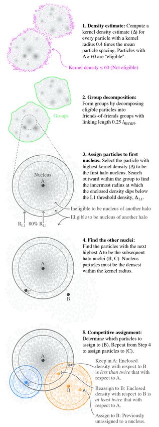
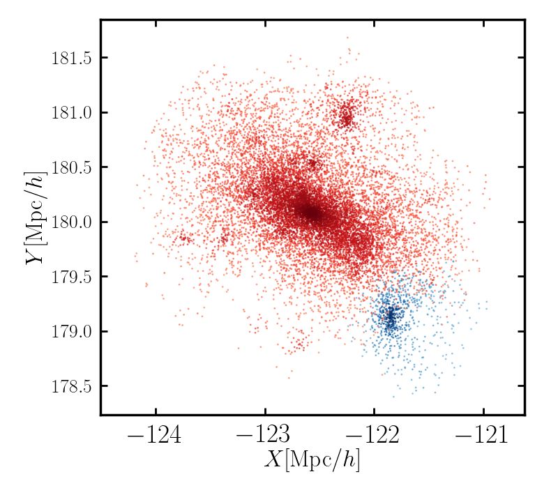
CompaSO 7

Figure 2. Scatter plots of haloes identified as “potential splits” (blue dots) and their central (largest) companions in the vicinity (red dots). The left panel shows
an example in which the “potentially split” halo does have a dense core, distinct from that of its companion. In this case, the smaller halo has been orbiting in
close proximity to the larger one for several snapshots (during which the algorithm has identified the two as a singular object) after which it has been expelled.
The right panel shows a case of a non-physical “potential split” for which the small halo is lacking a dense center of particles. A “potential split” is defined as an
object which in the previous time step, was considered part of a larger halo, but in the last time step, has been split by the CompaSO algorithm. Objects lacking
a well-defined core can be isolated by using diagnostics combining the merger tree flag IsPotentialSplit (see statistics for how often these occur in Table 2) and
the ratio of the radius containing all the particles to v,max (see Fig. 3). The scatter plots are using 3% of the halo particles.

the effects which contribute to their disruption and inconsistency
throughout the merger history are both physical as well as algorith- 6 CompaSO
mic. Smaller haloes are less likely to survive flybys past larger haloes
because their cores are less dense and thus more easily destructible. Potential splits
Another frequent interaction between a satellite and a central halo 5
is the expulsion of the satellite by the larger halo, which typically
 rhalo/rv,max

significantly reduces the mass of the expelled object, stripping it of
 4
its outermost layer. In addition, sometimes dark-matter substructure
on the outskirts of large haloes may have been identified as an au-
tonomous halo by the CompaSO algorithm at a given snapshot, but 3
this object might not have a distinct merger history. In this section,
we examine how often we find such occurrences by using statistics
output by the accompanying merger tree associations3 (Bose et al. 2
2021).
 In Fig. 2, we demonstrate two cases of haloes that have been
marked as “potential splits” (see Section 3.1 for a definition). On the 1013 1014
left panel, we show a case of a non-physical algorithmic split while Mhalo
on the right panel, the smaller halo has a healthy core and has only
spent a small portion of its history as part of its larger companion (but
otherwise has a distinct history). In Table 2, we show the percentage Figure 3. Ratio of the radius containing all halo particles to the radius where
of “potential splits” for different mass ranges in the third column. the maximum circular velocity is attained, v,max . We see that the haloes
We see that their numbers are very small in particular on the high- flagged as “potential splits” have a distinct halo / v,max distribution (blue
 shaded curve) compared with the typical CompaSO population (red shaded
mass end (log( ) > 13.7), where they are less than 0.004%. The
 curve). This indicates that looking at ratios of the inner and outer halo radii
overall percentage is around 12% and it is highly dominated by can help us diagnose problematic cases, since for these haloes their centers
the smallest haloes (log( ) ∼ 1011 ). The reason for this relatively are typically not correctly identified.
larger percentage is that for less massive objects flying through dense
regions, the boundary is harder to draw, as they have less dense cores
and are more difficult to distinguish from the background. This is
less and less frequent at higher halo masses. across longer periods of time. The simulation products include
 Another reliable diagnostic is to examine the persistence of haloes merger histories based upon stringing together consecutive snap-
 shots and thus obtaining a full merger tree, which we also dub as
 “fine.” Additionally, one can also utilise the “coarse” trees built over
3 These can also be found alongside the other products of the AbacusSummit non-adjacent time steps, spanning longer time epochs. To illustrate,
suite at https://abacussummit.readthedocs.io/en/latest/data-access.html the next two steps of the “coarse” merger trees for haloes at redshift of

 MNRAS 000, 1–21 (2019)

8 B. Hadzhiyska et al.

 log( ) range Number of haloes Main Prog. matching at = 0.875 Main Prog. matching at = 1.625 “Potential splits”
 11.5 ± 0.1 5096084 94.8% 73.1% 10.5%
 12.5 ± 0.1 610240 96.7% 91.4% 7.86%
 13.5 ± 0.1 46585 96.9% 89.9% 5.11%
 14.5 ± 0.3 2823 96.3% 85.3% 0.42%
 all haloes 24721876 89.7% 64.2% 12.8%

Table 2. Merger trees statistics for the haloes at = 0.5 using the AbacusSummit merger trees associations (Bose et al. 2021). The first two columns of the
table show the mass range selected as well as the number of CompaSO haloes in it at = 0.5. The next two columns show what percentage of these haloes’
main progenitors inferred through the “fine” tree associations agree with those inferred using the “coarse” tree ones at = 0.875 and = 1.625, respectively.
The last column displays what percentage of the haloes are identified as “potential splits” by the merger tree algorithm in each of the mass sets.

 = 0.5 are at = 0.875 and = 1.625. One of the “realness” criteria we opt not to perform particle unbinding because of both the speed
for the haloes at = 0.5 we propose is to compare their progenitors requirement of Abacus and the problems associated with it, some
at earlier times and note how often their “coarse” and “fine” histories of which we mention below. Instead, we adopt alternative strategies
point to the same progenitor. We do this at time steps = 0.875 and for cleaning the halo catalogues (see Section 3.1). In this section,
 = 1.625 and display the results in the first and second columns of we analyse the cleaned catalogues in terms of their effectiveness in
Table 2. At = 0.875, the progenitors of the haloes at = 0.5 match removing haloes with a large presence of high-velocity (“unbound”)
at & 95% at the mass scales typically of interest for creating mock particles. We verify that indeed after the cleaning, very few problem-
catalogues (i.e. log( ) ∼ 11.5 and higher) and close to 90% for atic haloes remain in the catalogues. In addition, we find alternative
the entire halo population. haloes for which we find a match can be statistics that help us weed out unphysical haloes that were missed in
certified as “healthy,” though we should not be discarding those for the cleaning.
which no match, as there could be multiple reasons for this (e.g., a Energy-based unbinding is typically done to discard particles that
halo has orbited inside a larger companion for a significant portion of are tentatively assigned to a particular (sub)structure, but do not ap-
its life and as a result has lost a substantial amount of mass, which has pear gravitationally bound to it. For subhaloes, removing unbound
caused the step-by-step merger tree to fail at tracing its history). At particles is of particular importance, since their particle lists are often
 = 1.625, the percentages are noticeably lower. For the high-mass contaminated with particles from the host halo due to the relatively
objects, they are close to 90%. However, we note that on the low-mass lower density of the subhalo. This can influence significantly the
end, oftentimes the haloes have not yet been formed at these earlier inferred subhalo properties such as its mass and dispersion veloc-
redshifts, so the merger tree “fine”-to-“coarse” comparison might not ity. Similarly, interacting haloes often acquire stray particles whose
be an accurate test of persistence. velocities are too high to keep them bound to their host. Standard
 There are potentially other ways to spot and diagnose unphysical unbinding treats every halo individually and removes all particles
haloes. As mentioned above, some objects are identified by the Com- whose kinetic energies exceed their potential energy.
paSO algorithm as distinct haloes while in reality they may lack a
 However, there are several well-known issues associated with
dense core and might simply be carved out of a nearby companion
 energy-based unbinding. The presence of particles with high ve-
due to the SO boundary. For these objects, the ratio between radial
 locities inside the boundaries of the halo is often a consequence of
quantities such as halo and v,max will most likely be atypical com-
 close fly-bys with other haloes. Therefore, the high-velocity parti-
pared with the rest of the population at that mass scale. In Fig. 3,
 cles should instead be assigned to a neighbour (which is also the
we demonstrate what the distribution looks like for haloes flagged
 spirit of the competitive assignment algorithm for CompaSO and
as “potential splits” by the merger tree algorithm and the rest of the
 the cleaning procedure). In standard unbinding, these particles are
population. We can notice that the ratios are particularly different for
 usually returned to the next level up the halo hierarchy, but when ap-
the lower halo masses, which is also where we expect to find most
 plying unbinding to halo hosts, the unbound are altogether deprived
of the unphysical algorithmic choices. On the higher mass end, the
 of halo membership rather than merged onto a close neighbour. The
“potential splits” are more consistent with the general population.
 unbinding procedure assumes that the halo is isolated, and any ef-
As discussed, some of the objects labelled “potential splits” may in
 fects that arise from outside, e.g. particles on the edges, interactions,
fact be “real” haloes expelled after orbiting a companion halo (par-
 tidal effects, are neglected. In particular, even particles in isolated
ticularly for haloes with denser cores and more particles), so a more
 haloes whose orbits take them outside of the arbitrarily defined “halo
robust way of “pruning” the merger tree would involve flagging ob-
 radius” have their ability to return underestimated because the mass
jects with odd ratios of their radial quantities which have also been
 contribution from the particles outside is neglected (we address this
identified as “splits.”
 below). In addition, in the case of interacting haloes (e.g, two haloes
 orbiting around each other, or falling into each other), calculating
 the potential of each particle with respect to a single halo would not
3.3 Presence of high-velocity particles
 be reflective of the gravitational forces experienced by the particle.
A problematic mode for many halo finders is the deblending of close Enlarging the scope and considering the global potential of the sim-
pairs of haloes with a large mass ratio, where particles get assigned ulation, on the other hand, is also not the correct quantity to use,
to one halo, even though they may not be bound to that halo. Neglect- as it is large-scale dominated and does not answer the question of
ing the presence of these particles may bias the inferred properties whether the particle is bound to a particular halo. The simplification
of the haloes such as their spins and velocity dispersions. A way of ignoring interactions is also motivated by the enormous computa-
to identify such failed cases is by locating particles with high infall tional expense that would arise from taking the entirety of structures
velocities. Some configuration-space-based finders address this issue in the computational domain into account for each structure anew. A
by performing energy-based unbinding, but in the case of CompaSO, more precise approach involves boosting the gravitational potential

MNRAS 000, 1–21 (2019)

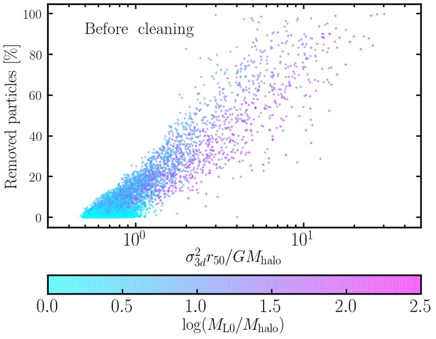
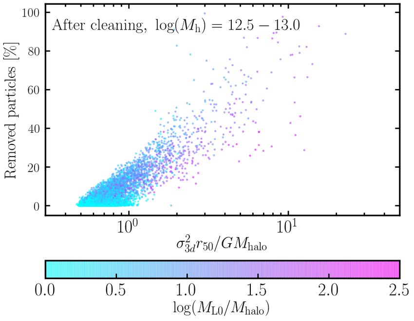
CompaSO 9
to make it a locally meaningful quantity, which can be used to define
 2.5
a binding criterion that incorporates the effect of tidal fields (Stücker f (c) = [ln(1 + c)(c−1 + 1) − 1]−1
et al. 2021).
 We test the effect of applying energy-based unbinding to the 2.0
CompaSO catalogues of a small test simulation with box size
 M∗

 f (c)
 box = 296 Mpc/ℎ and particle mass part = 2.1 × 109 /ℎ, 1.5
containing 1.3 million haloes. We also apply the ‘cleaning’ proce-
dure from Section 3.1 and Bose et al. (2021), which identifies 1.6%,
or 21000, of the haloes in the simulation as ‘unphysical’. We per-
 1.0
form the process of unbinding iteratively for each halo in its centre
of momentum frame of its core, i.e. subtracting xL2com and vL2com 0.5
from the position and velocity of each particle, x and v. All comoving
positions are converted into proper coordinates, and the Hubble flow
term is added to the particle velocities, ( )( − L2com ). We com-
 100 101 102
pute the spline potential adopted by Abacus (Garrison et al. 2021) at
 c
each iteration, discarding the particles with kinetic energies higher
than their potential energies. This process continues until no more Figure 4. Factor ( ) determining the magnitude of the extra potential term
particles are found to be unbound. as a function of concentration, as derived in Eq. 5. Less concentrated haloes
 In addition, we propose a simple, yet well-motivated modification receive a larger contribution to their potentials from particles lying outside vir
to the standard unbinding algorithm, which ameliorates the issue of compared with more highly concentrated haloes. The black vertical dashed
the arbitrary drawing of halo boundaries. Let us imagine an isolated line shows roughly the concentration of Mily-Way-like haloes. We note that
 halo concentration and halo mass are weakly anti-correlated.
halo whose density profile follows an NFW distribution. Typically,
we define the halo boundaries, vir , by requesting that the enclosed
density is × crit . In the case of CompaSO, the ‘virial mass’ is
defined using the Bryan & Norman (1998) scaling relation (see Sec- percentage of removed particles and the haloes that were cleaned
tion 2.3). Nevertheless, the particles outside vir still contribute to away. To test this, in the middle panel, we show the cumulative
deepening the potential well of the halo despite not strictly belonging percentage of haloes with more than X% “unbound particles” for
to it. Not accounting for this outside contribution would lead us to three mass bins and find that the majority of haloes have less than
falsely discard bound particles that, as a result of the deepening of the 0.1% removed particles, with higher mass bins performing better.
potential, are in thermal equilibrium despite their higher velocities. Overall, as also illustrated in the bottom of Fig. 5, the cleaning makes
This extra contribution to the potential, extra , assuming a spherical a big difference, removing very effectively haloes that have more
halo, is computed below for an NFW profile. than 10% “unbound particles”. For the higher masses, the cleaning
 ∫ ∞ is even more efficient and removes up to 100% of the haloes with
 4 NFW ( ) 2 vir /( + 1)
 extra = = − , (4) a large unbound particle population. If the cleaning procedure from
 vir vir NFW Section 3.1 is regarded as reliable, then this finding suggests that the
where NFW ≡ ln (1 + ) − /(1 + ), ≡ / vir , and is the halo unbinding procedure augmented with an extra potential term yields
concentration. Simplifying this, we get: a more robust halo catalogue compared with the standard unbinding
 procedure.
 vir vir
 extra = − [ln(1 + )( −1 + 1) − 1] −1 ≡ − ( ) (5) In addition, we test the conjecture that unphysical objects (e.g.,
 vir vir
 haloes with a bimodal profile or haloes lacking a nucleus) can be
 and show the function ( ) in Fig. 4. We note that in the case of identified through other internal halo properties that are already be-
elliptical haloes, the assumption of spherical shapes tends to un- ing output. In Fig. 6, we consider two such quantities. The first one is
derestimate the contribution of the outside potential and its ability 2 / , where 
 the virial ratio 3 50 vir 3 is the three-dimensional
to stabilise the particles on the edges of the halo. Nevertheless, to dispersion velocity. Fig. 6 indicates that there is a very strong corre-
approximately account for this effect, we add the term extra to the lation between haloes with a large percentage of unbound particles
potential energy of each halo when removing unbound particles. As and a large virial ratio. One can therefore imagine augmenting the
demonstrated in Fig. 8, the truncated NFW profile is a good ap- cleaning procedure with a requirement that the halo virial ratio does
proximation to the CompaSO halo profiles. We thus obtain the halo not exceed a certain threshold such as 2 or 3, which as seen in the
concentration by fitting an NFW profile to every halo. For haloes figure for the bin log( halo ) = 12.5 − 13.0, gets rid of the major-
for which a fit cannot be obtained (mostly small haloes, making up ity of offenders. In fact, after performing the cleaning, only 1.14%
less than 3%), we approximate the concentration as 100 / 10 . of the haloes with mass log( halo ) = 11.5 − 12.0, 0.63% of the
 In the top panel of Fig. 5, we show the averaged percentage of haloes with mass log( halo ) = 12.0 − 12.5, 0.37% of the haloes
removed particles as a function of halo mass when we apply the with mass log( halo ) = 12.5 − 13.0, 0.19% of the haloes with
standard unbinding procedure and the extra -augmented procedure mass log( halo ) = 13.0 − 13.5, 0.038% of the haloes with mass
(see Eq. 5). We see that the standard procedure removes 6.5% of the log( halo ) = 13.5 − 14.0, and none above log( halo ) = 14.0, are
particles in smaller haloes and 4% of the particles in higher-mass retained that have virial ratio above 3. All masses are reported in
haloes. These number are significantly reduced when including the units of /ℎ.
 extra term, to 3.5% and 0%. Additionally, we discard the haloes We conjecture that this is due to issues that CompaSO has with de-
considered ‘unphysical’ by the cleaning procedure of Section 3.1 blending haloes in close proximity and in particular, with determining
and Bose et al. (2021), noting that the average percentage of removed the boundaries of small haloes near larger ones. To test this, we have
particles is brought down by nearly 1-2% for halo < 1014 /ℎ. colour-coded the points in Fig. 6 by the logarithmic ratio of the “L0”
This implies that there is an overlap between haloes with a large parent group mass and the halo mass, log( L0 / halo ), with small

 MNRAS 000, 1–21 (2019)

10 B. Hadzhiyska et al.

 12 Unbinding, standard (before cleaning)
Removed particles [%]

 10 Unbinding, standard (after cleaning)
 Unbinding, extra potential (before cleaning)
 8 Unbinding, extra potential (after cleaning)
 6

 4

 2

 0
 1011 1012 1013 1014 1015
 Mhalo [M /h]
 40
Percentage haloes w/ ≥ X% removed

 Before cleaning
 After cleaning
 30 log Mh = 11.3 − 11.8
 log Mh = 12.3 − 12.8
 log Mh = 13.3 − 13.8
 20

 10

 0
 10−1 100 101 102
 Removed particles [%]
Discarded after cleaning [%]

 100
 log Mh = 11.3 − 11.8
 75 log Mh = 12.3 − 12.8
 log Mh = 13.3 − 13.8
 Percentage haloes [%]

 50 Before cleaning
 101 After cleaning
 25
 100
 0
 10−1 100 101 102
 10−1
 Removed particles [%]
 0.37%
Figure 5. Top panel: Average percentage of removed particles through un- 100 101
 2
binding as a function of halo mass. In blue, we show the result when per- σ3d r50/GMhalo
forming the standard cleaning procedure (see Section 3.1 and Bose et al.
(2021)), whereas in red, we show the outcome when adding an extra term
to the potential energy, extra (see Eq. 5). The percentage of removed parti- Figure 6. Coloured scatter plot of the percentage of removed particles
cles is significantly reduced (top panel) when including extra – by a factor due to unbinding as a function of the virialisation parameter, defined as
 2 / 
of ∼ 2 for smaller haloes and ∼ 10 for higher-mass haloes. Similarly, when 3 50 halo . The colour denotes the ratio of the mass of the “L0” parent
we remove the discarded haloes (dashed lines), the average percentage of group and the halo mass, log( L0 / halo ), with purple corresponding to a
removed haloes drops further. The objects that are cleaned away make up high ratio and blue corresponding to a low ratio. The plot shows all haloes
1.6% of all haloes in the simulation. Middle panel: Cumulative percentage of in the range log halo = 12.5 − 13.0, measured in units of /ℎ, before
haloes as a function of removed particles before and after cleaning for three applying the cleaning procedure (top panel) and after (middle panel). We see
different mass bins: log( halo ) = 11.3 − 11.8, log( halo ) = 12.3 − 12.8, a strong positive correlation between the virialisation ratio and the percent-
and log( halo ) = 13.3 − 13.8. We see that 38%, 36% and 30% of the before- age of removed particles, suggesting that a viable mechanism for cleaning
cleaning haloes for these mass bins have more than 0.1% of their particles the halo catalogues in addition to the default CompaSO cleaning may involve
removed, while 10%, 7% and 3$, respectively, have more than 10% removed. discarding haloes with a high virialisation parameter (& 2-3). Furthermore,
The cleaning reduces these numbers by several per cent. Bottom panel: Per- haloes with a high ratio log( L0 / halo ) tend to lose a higher percentage
centage of retained haloes after cleaning as a function of removed particles of their particles to unbinding, indicating that the most problematic mode of
for three different mass bins. It is encouraging to see that the cleaning weeds CompaSO is the assignment of particles to haloes in a cluster. In the bottom
out an increasingly larger number of haloes (close to 100% for the highest panel, we show the percentage of haloes as a function of virial ratio before
mass bin shown), as we consider haloes with an increasingly large number of and after cleaning. Haloes to the right of the dashed black line account for
“unbound” particles. 0.37% of all haloes after cleaning in the mass bin. This demonstrates that the
MNRAS 000, 1–21 (2019) cleaning takes care of the majority of bad actors and leftover objects can be
 discarded by combining output statistics such as the virialisation parameter
 and the cluster mass ratio.