A convolutional neural network for classifying cloud particles recorded by imaging probes - AMT
←
→
Page content transcription
If your browser does not render page correctly, please read the page content below
Atmos. Meas. Tech., 13, 2219–2239, 2020
https://doi.org/10.5194/amt-13-2219-2020
© Author(s) 2020. This work is distributed under
the Creative Commons Attribution 4.0 License.

A convolutional neural network for classifying cloud particles
recorded by imaging probes
Georgios Touloupas1, , Annika Lauber2, , Jan Henneberger2 , Alexander Beck2 , and Aurélien Lucchi1
1 Institute
         for Machine Learning, ETH Zurich, Zurich, Switzerland
2 Institute
         for Atmospheric and Climate Science, ETH Zurich, Zurich, Switzerland
 These authors contributed equally to this work.

Correspondence: Annika Lauber (annika.lauber@env.ethz.ch) and Jan Henneberger (jan.henneberger@env.ethz.ch)

Received: 17 May 2019 – Discussion started: 15 July 2019
Revised: 11 November 2019 – Accepted: 5 March 2020 – Published: 8 May 2020

Abstract. During typical field campaigns, millions of cloud      1   Introduction
particle images are captured with imaging probes. Our in-
terest lies in classifying these particles in order to compute   Clouds play an important role in our weather and climate sys-
the statistics needed for understanding clouds. Given the        tem. Nevertheless, our understanding of microphysical pro-
large volume of collected data, this raises the need for an      cesses, especially in mixed-phase clouds (MPCs), which are
automated classification approach. Traditional classification    a large source of precipitation in the mid-latitudes (Mülmen-
methods that require extracting features manually (e.g., de-     städt et al., 2015), is limited (Boucher et al., 2013; Korolev
cision trees and support vector machines) show reasonable        et al., 2017). Global climate models and satellite-based ob-
performance when trained and tested on data coming from a        servations show a large spread in the fraction of ice and
unique dataset. However, they often have difficulties in gen-    supercooled liquid in MPCs (McCoy et al., 2016). Phase-
eralizing to test sets coming from other datasets where the      resolved in situ observations can constrain the phase parti-
distribution of the features might be significantly different.   tioning in MPCs (Baumgardner et al., 2017). Furthermore,
In practice, we found that for holographic imagers each new      phase-resolved observations of MPCs are crucial to improve
dataset requires labeling a huge amount of data by hand using    the understanding of processes like primary and secondary
those methods. Convolutional neural networks have the po-        ice production. Yet, in particular, the measurements of ice
tential to overcome this problem due to their ability to learn   crystals below 100 µm remain a challenge (Baumgardner
complex nonlinear models directly from the images instead        et al., 2017).
of pre-engineered features, as well as by relying on powerful       For single-particle detection, there are two common mea-
regularization techniques. We show empirically that a convo-     surement instruments: imaging and light scattering probes.
lutional neural network trained on cloud particles from holo-    The latter (e.g., small ice detector – SID-2 – in Cotton et al.,
graphic imagers generalizes well to unseen datasets. More-       2010; backscatter cloud probe – BCP – in Beswick et al.,
over, fine tuning the same network with a small number           2014; cloud, aerosol and precipitation spectrometer – CAS –
(256) of training images improves the classification accuracy.   in Baumgardner et al., 2001) capture the scattered light of a
Thus, the automated classification with a convolutional neu-     single particle usually over a range of angles. Applying Mie
ral network not only reduces the hand-labeling effort for new    theory and scale factors, which are derived from calibrations,
datasets but is also no longer the main error source for the     information about the measured particle like the equivalent
classification of small particles.                               optical diameter (EOD) can be derived. However, this can be
                                                                 a major issue for nonspherical ice crystals, since the deriva-
                                                                 tion of the EOD assumes sphericity, and the exact shape of
                                                                 the captured particle is unknown (Baumgardner et al., 2017).

Published by Copernicus Publications on behalf of the European Geosciences Union.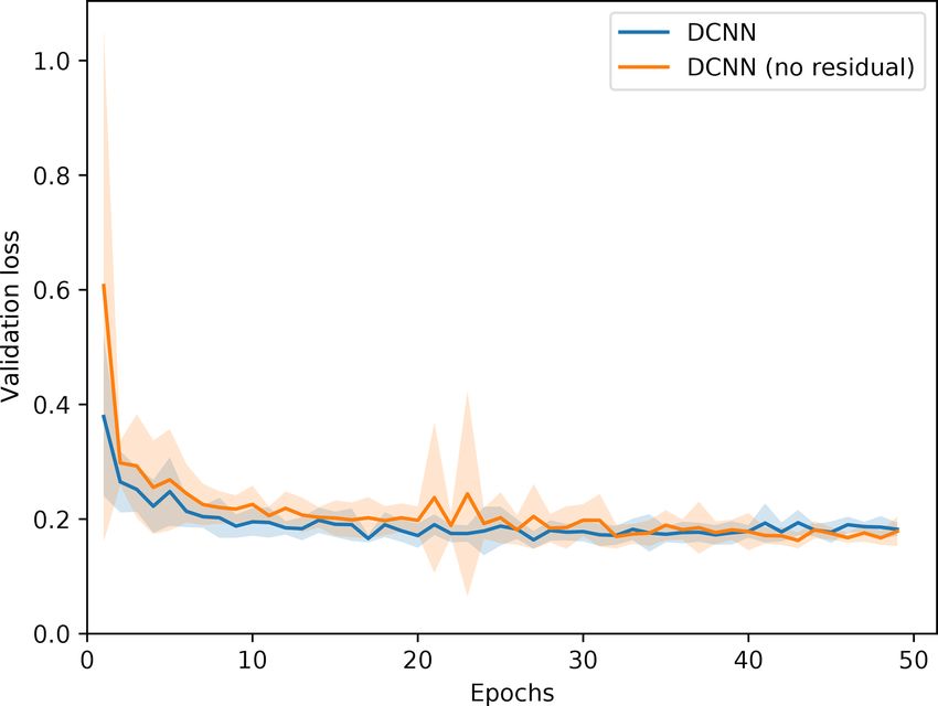
2220                                                                G. Touloupas et al.: A CNN for classifying cloud particles

   This issue is partly overcome with imaging probes, which         the existing approaches are not suitable for holographic im-
capture images of the particle itself. Assumptions about the        ages, since they do not account for artifacts. Finding good
shape have only to be made on the third dimension and if            features for artifacts is difficult because they do not have a
the resolution is low compared to the particle size like that       specific shape.
outlined later in this section. While cloud particle imaging           Therefore, classification methods that are commonly used
probes like the CPI (cloud particle imager; Lawson et al.,          for holographic imagers rely on supervised machine learning
2001), CIP (cloud imaging probe; Baumgardner et al., 2001)          approaches which learn to predict labels (a.k.a. classes) from
and PHIPS-HALO (Particle Habit Imaging and Polar Scat-              labeled training data. The algorithm is trained with input
tering probe; Abdelmonem et al., 2011, 2016) directly cap-          samples, called training data, which were labeled by humans
ture a 2D particle image of single cloud particles, digital         (i.e., hand-labeled) into a defined number of classes. For ex-
in-line holography (e.g., Holographic Detector for Clouds –         ample, the images can be divided into three classes, namely
HOLODEC – in Fugal and Shaw, 2009; HOLographic Im-                  liquid droplet, ice crystal and artifact. Many supervised ma-
ager for Microscopic Objects II – HOLIMO 2 – in Hen-                chine learning algorithms cannot directly handle particle im-
neberger et al., 2013; HOLIMO 3G in Beck et al., 2017; and          ages as inputs, but instead they require extracting a set of
HALOHolo in Schlenczek, 2018) captures the information              features from the images (e.g., sphericity and area). The per-
about an ensemble of cloud particles on a so-called holo-           formance of the algorithm describes how well these features
gram. From such a hologram 2D particle images of the ob-            can distinguish between the different classes. For instance,
served cloud particles are computationally reconstructed (see       decision trees and support vector machines (SVMs), which
Sect. 2). Based on these particle images, both techniques           were used for the classification of ice crystal shapes by Grazi-
offer information about the shape, size and concentration           oli et al. (2014) and Bernauer et al. (2016), use around 10 to
of cloud particles. The phase of cloud particles can be de-         30 extracted features as the input. Although these algorithms
termined by distinguishing between circular-shaped liquid           might achieve reasonable results when trained and tested on
droplets and non-circular-shaped ice crystals (Baumgardner          a single dataset, they often have difficulties in generalizing
et al., 2017). In addition, the particle images can be used         to different datasets whose features might follow a slightly
to classify different ice crystal habits (e.g., Lindqvist et al.,   different distribution. This problem is commonly referred to
2012). The differentiation of liquid droplets and ice crystals      as transfer learning in the machine learning community (see
by their shapes requires a minimum diameter which depends           details in Goodfellow et al., 2016).
on the complexity of the ice crystal. To identify needles, six         Deep learning (usually referred to as neural networks) has
pixels might be enough, whereas a minimum of 12 to 15 pix-          the potential to overcome transfer learning issues, which we
els is required to identify plates, while frozen droplets which     will show in this work. For the classification of cloud par-
are spherical cannot be detected regardless of their diameter       ticles, a feedforward neural network from Hagan and Men-
(Korolev and Sussman, 2000; Korolev et al., 2017).                  haj (1994) was used by O’Shea et al. (2016) to classify CPI
   During a typical field campaign, millions of images of           data into different ice particle shapes and liquid droplets. The
cloud particles are captured. For phase-resolved measure-           network is fed by different features, which are calculated be-
ments in MPCs, the cloud particles need to be classified into       forehand. Their results are promising with a total accuracy
liquid droplets, ice crystals and, in the case of holography,       of 88 % for classifying the images into six habits including
also artifacts, which are usually part of the interference pat-     liquid droplets for particles larger than 50 µm. This type of a
terns of larger particles (more details in Sect. 2). The clas-      neural network also requires feature extraction and does not
sification of such a large amount of images by hand is a            work for holographic images, because it does not account for
very time-consuming step, which raises the need for an auto-        a class without a specific shape like artifacts.
mated classification algorithm. Because ice crystals are very          In this paper, we suggest using a convolutional neural
variable in shape and their typical maximum dimensions of           network instead, which does not require any manual fea-
about 1–1500 µm overlap with the size range of cloud and            ture extraction but can instead use the particle images as in-
rain droplets (about 1 µm to a few millimeters) together with       puts directly. Automatically extracting features from image
artifacts, which can have any shape and size, it is difficult to    data allows for more reliable and robust predictions to be
develop a classification algorithm to perform well.                 made, which we will demonstrate empirically. Our experi-
   Imaging probes, which differentiate only ice from liquid,        mental setup consists of training a convolutional neural net-
usually extract features from the images that measure the cir-      work (CNN) on several real-world datasets of cloud particles
cularity of the particles (e.g., Korolev and Sussman, 2000;         with major-axis sizes larger than 25 µm (see Sect. 2) recorded
Crosier et al., 2011; Lawson et al., 2001). Korolev and Suss-       by different holographic imagers. This technique achieves
man (2000) state that there is an uncertainty for differenti-       higher accuracy and exceeds the generalization abilities of a
ating spheres from irregular particles of 20 % to 25 % for a        decision tree and SVM baseline (see Sect. 4.4). Nevertheless,
pixel number between 20 and 60 and a few percent for higher         we still have to account for varying accuracy over particle
pixel numbers. These values are comparable to our results for       size (see Sect. 4.5). We also introduce a fine tuning approach
holographic images, which we will introduce later. However,

Atmos. Meas. Tech., 13, 2219–2239, 2020                                               www.atmos-meas-tech.net/13/2219/2020/
G. Touloupas et al.: A CNN for classifying cloud particles                                                                       2221

Figure 1. Working principle of digital in-line holography. The laser
is collimated by a convex lens. Particles between the lens and the
camera scatter the light which interferes with the plane reference     Figure 2. Channels computed from an ice crystal complex image.
wave. The interference pattern is captured by the camera as a holo-    (a) Amplitude channel. (b) Phase channel.
gram from which images at different distances to the camera can be
reconstructed. Figure adapted from Beck et al. (2017).

                                                                       the CNN, only the amplitude and phase images of the focus
that can significantly improve the performance of the CNN              plane were used.
(see Sect. 4.2).                                                          Five different hand-labeled datasets from two different in-
                                                                       struments (HOLIMO 3M and HOLIMO 3G; Beck et al.,
                                                                       2017) were used for testing and training. The datasets were
2   Experimental data                                                  obtained at different measurement sites in different weather
                                                                       situations and were labeled by different people (Table 1).
The data used for training and validation of the classification           The class distributions vary strongly between the datasets,
algorithms presented in this paper were obtained in situ with          which is due to different environmental conditions but also
several holographic imagers utilizing digital in-line holog-           to different preprocessing routines of the data (Table 1). For
raphy. For this technique, a laser irradiates an ensemble of           example, a lower-amplitude threshold for particle detection
particles inside a cloud volume. The particles in this cloud           during the reconstruction results in a larger fraction of arti-
volume scatter the laser light, and the scattered wavefronts           facts. Furthermore, the more particles inside a measurement
interfere with the unscattered laser beam. The resulting in-           volume there are, the lower the signal-to-noise ratio is, and
terference pattern (hologram) is captured by a digital cam-            the higher the number of artifacts is. The pixel intensity dis-
era (see Fig. 1). From the hologram, 2D complex images are             tributions of the datasets give an indication of their different
numerically reconstructed at several planes within the cloud           noise levels. Because the distributions differ substantially be-
volume of a regular distance (usually 100 µm) using the soft-          tween the datasets (see Appendix B), it has been difficult to
ware HOLOSuite (modified version of Fugal et al., 2009)                develop an automated classification algorithm working for
and are depicted as amplitude and phase images (see Fig. 2).           all of them.
The software then detects images of the particles in different            The classes predicted by the CNN were evaluated against
planes within the reconstructed amplitude images by using              the hand-labeled classes, which are considered as the ground
an amplitude threshold and patches the images of the par-              truth. Nevertheless, some particles in the training datasets
ticles in adjacent planes which are at the same lateral posi-          can also have a wrong class or label. Because the classifi-
tion. Patched traces are assumed to be one particle. The focus         cation was done by humans, misclassification can have hap-
planes of particles within particle patches are determined by          pened by accidentally pressing the wrong button or by misin-
using an edge sharpness algorithm. A more detailed descrip-            terpreting the image. In some cases, it is not possible to dis-
tion of the measurement technique and software can be found            tinguish between two classes, e.g., circular or very small ice
in Henneberger et al. (2013) and Fugal et al. (2009).                  crystals cannot be separated from liquid droplets. In addition,
   To reduce the amount of data, only the particle pixels              optical distortion compromises the classification. Particles
and a few pixels of their surrounding were saved for the               far away from the camera have a blurry edge as the resolution
subsequent analyses. The data were hand-labeled into three             gets worse, and at the edges, the lens distortion deforms cir-
classes: liquid droplets (circular particles), ice crystals (non-      cular particle to an oval shape. The training dataset was con-
circular particles) and artifacts (parts of the interference pat-      strained to particles with a major-axis size larger than 25 µm,
tern, scratches on the windows, noise, etc.). The decision was         corresponding to 8 pixels, which is the empirical threshold
usually made based on the amplitude images in the focus                from which a reliable determination of the classes for most
and its neighboring planes, but also the traces of the am-             of the particles is possible.
plitude images within a particle patch (like the gradients of             For the estimation of the human bias, three different peo-
the maximum and minimum values) provide useful informa-                ple hand-labeled the same dataset consisting of 1000 parti-
tion. Traces of artifacts are rather fluctuating, while traces         cles. The number of particles hand-labeled as the considered
of particles show a clear maximum. For training and testing            class by at least one person is compared to the number of par-

www.atmos-meas-tech.net/13/2219/2020/                                                    Atmos. Meas. Tech., 13, 2219–2239, 2020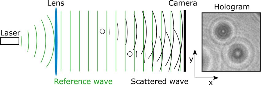
2222                                                                    G. Touloupas et al.: A CNN for classifying cloud particles

Table 1. Detailed information on the different datasets used for training and testing the CNN. The ’i’ in iHOLIMO stands for intercomparison,
as the datasets were collected to compare the HOLIMO 3G and HOLIMO 3M instruments. “JFJ” denotes Jungfraujoch and “SON” denotes
Sonnblick, which were the measurement sites for the datasets.

    Dataset         Instrument      Location                    Date               Total    Liquid         Ice   Artifacts   Labeled by
                                                                                   (no.)   droplets   crystals       (no.)
                                                                                              (no.)      (no.)
    iHOLIMO 3G      HOLIMO 3G       Jungfraujoch, Switzerland   November 2016     22 373    17 547        894       3932     Annika Lauber
    iHOLIMO 3M      HOLIMO 3M       Jungfraujoch, Switzerland   November 2016     20 253     4166         393      15 694    Sarah Barr
    JFJ 2016        HOLIMO 3G       Jungfraujoch, Switzerland   March 2016         7221      1744         516       4961     Jan Henneberger
    SON 2016        HOLIMO 3G       Hoher Sonnblick, Austria    March 2016        15 648     7056       2215        6377     Alexander Beck
    SON 2017        HOLIMO 3G       Hoher Sonnblick, Austria    February 2017     19 476       151     17 453       1872     Alexander Beck

                                                                         iar with deep learning to Appendix A, where they can find a
                                                                         general introduction about deep CNNs.

                                                                         3.1     Network architecture

                                                                         The CNN used during this work was adapted from the
                                                                         VGG (Visual Geometry Group) architecture of Simonyan
                                                                         and Zisserman (2014), as shown in Fig. 4. The first part of
                                                                         the architecture consists of multiple convolutional blocks,
                                                                         each having two or three convolutional layers followed by
                                                                         a max-pooling layer. The architecture was adjusted to accept
                                                                         32 × 32 × 2 pixels (amplitude and phase images) as inputs.
                                                                         For the convolutional part of the CNN, four convolutional
                                                                         blocks are used, with the first two containing two convolu-
                                                                         tional layers and the next two containing three convolutional
Figure 3. Evaluation of the human classification bias from three         layers. The convolutional layers use 3 × 3 filters with stride
people labeling the same dataset consisting of 1000 particles. The       S = 1, zero padding and ReLUs (rectified linear units) as the
upward pointing triangles are the total number of particles labeled      activation functions. The number of filters is the same for all
by all three people as the considered class (100 % agreement). The       convolutional layers inside the same convolutional block and
downward pointing triangles are the total number of particles clas-      increases throughout the convolutional part of the network,
sified by at least one person as the considered class (≥ 33 % agree-     from 64 to 128, 256 and eventually 512. The pooling layers
ment). The diamond is the average between the two points with the        perform max pooling with stride S = 2, each one reducing
percentage values as the deviation to them.                              the spatial dimensions by two. In total, 2048 features are ex-
                                                                         tracted in the convolutional blocks.
                                                                            For the classifier part of the network, three fully connected
ticles hand-labeled as the considered class by all three peo-            layers progressively reduce the dimensions from 1024 to 128
ple. Taking the average of these two numbers, the spread can             to 3 (artifact, liquid droplet and ice crystal). A ReLU is also
be given as the percentage deviation to the two values (see              used as the activation function for the fully connected layers.
Fig. 3). We have a deviation for liquid droplets of ±4 % and                To speed up training, dense residual connections are used
for ice crystals of ±5 %. However, this estimation does not              (Huang et al., 2017). Inside each convolutional block, con-
take into account that in some cases humans might just not               nections from every layer to all the following layers were
be able to recognize the correct class as outlined before.               added. Similarly to He et al. (2016), batch normalization is
                                                                         also performed right after each convolutional and fully con-
                                                                         nected layer and before the ReLU activations, as well as after
                                                                         the pooling layers and the input layer.
3   Network architecture, implementation and
    evaluation method                                                    3.2     Data preprocessing

In this section, we discuss the architecture of the CNN used             3.2.1    Normalizing the input
in our experiments and provide details about the training pro-
cedure as well as the fine tuning method. We also introduce              The images were preprocessed to a standard format before
the baselines used for comparison. We refer readers unfamil-             being given to the CNN (Fig. 5). Standard CNN architectures

Atmos. Meas. Tech., 13, 2219–2239, 2020                                                      www.atmos-meas-tech.net/13/2219/2020/
G. Touloupas et al.: A CNN for classifying cloud particles                                                                              2223

Figure 4. The VGG-based CNN architecture. Two preprocessed images (amplitude and phase) of a combined canonical size of 32 × 32 × 2
pixels are fed to the CNN architecture, which consists of a sequence of layers that implement various operations (see the detailed description
of each operation in Appendix C). The CNN processes the input image and outputs probabilities for each of the three classes considered
here. The class with the highest probability is then chosen as the prediction (the class with the green border in this figure with a softmax
probability of 0.83). Figure adapted from Cord (2016).

(including VGG) require a fixed square size image as the in-             transformations could have been applied to one image during
put. The size of the input image is a design choice that is typi-        training. This process was switched off after training.
cally determined by various restrictions. While larger images
slow down training and increase the amount of memory re-                 3.3    Training details
quired by the network, smaller input images reduce the reso-
lution and therefore the information available in the images.            The weight parameters of the network were initialized using
We empirically found that using an image size of 32 × 32                 the Xavier initialization scheme (Glorot and Bengio, 2010),
pixels leads to satisfying results. These images were created            while all biases were initialized to 0.1. The loss function
as follows. From the raw complex image data (see Sect. 2),               (see Appendix A2) used to train the network is a softmax
both the amplitude and phase images were extracted. Square               cross-entropy method which was modified to combat the is-
images were created by filling the unknown pixel values with             sue of having imbalanced classes. This problem arises when
black pixels (zero padding) and scaling the images to 32×32              a dataset contains significantly more labels of one class com-
pixels. The amplitude and phase images were fed to the CNN               pared to the other classes. Since the cross-entropy loss penal-
as two different channels.                                               izes the misclassification of all classes equally, the learned
                                                                         model will be biased towards the class with the highest class
                                                                         frequency. To avoid this behavior, the importance of each
3.2.2   Data augmentation
                                                                         class in the cross-entropy loss was weighted by its inverse
                                                                         class frequency. This reweighting results in an increase in
Techniques such as data augmentation help a CNN to achieve               performance for the rarer classes. In order to optimize the
lower generalization errors (measure of how accurately an al-            weights of the network, a variant of stochastic gradient de-
gorithm is able to predict outcome values for previously un-             scent named Adam (Kingma and Ba, 2014) was used. The
seen data), especially when the amount of data available for             learning rate was set to η = 10−3 , and the gradients were
training is limited. We augmented the training data by per-              computed using mini-batches of 256 samples.
forming transformations that preserve the shape of the par-                 In order to prevent overfitting to the training set, which
ticles such as vertical flip, horizontal flip, 90◦ rotation and          would increase the generalization error, a separate validation
transposition (see Fig. 6). Each transformation was applied              set was used to select the best set of parameters. This set
with a 50 % probability to every input image before it was               was created by splitting the data available for training (not
fed to the network during training. This means that multiple             including data for testing) into a training set and a validation

www.atmos-meas-tech.net/13/2219/2020/                                                        Atmos. Meas. Tech., 13, 2219–2239, 2020
2224 G. Touloupas et al.: A CNN for classifying cloud particles
Figure 5. Preprocessing steps for an ice crystal image (only the amplitude channel is shown). (a) Original image of 89 × 63 pixels. (b) Zero-
padded square image of 89 × 89 pixels. (c) Scaled image of 32 × 32 pixels used as an input to the network.
Figure 6. Data augmentation transformations applied on an ice crystal image; visualization of the amplitude channel. The transformations
are applied to the original image: (a) original image, (b) vertical flip, (c) horizontal flip, (d) 90◦ rotation and (e) transposition.
set. The training set was used for training the network as de- 3.4 Fine tuning
scribed so far, whereas the validation set was used to evalu-
ate the performance of the network on unseen data. Typically Using the CNN trained on a dataset with different character-
the loss of the network for the training set decreases steadily istics from the target dataset may lead to less good or even
during training, while the loss on the validation set will start poor results. A fine tuning approach that reuses the weights
to increase after a certain point. This is a sign that the net- of the pre-trained CNN as the initialization for a model be-
work starts to overfit to the training set, and therefore the ing trained on a sample of the target set may overcome this
training was stopped (this method is referred to as early stop- issue. This approach requires only a low number of training
ping). In our implementation, the loss of the validation set samples to be powerful (a few hundred as explained later),
was computed after each epoch (one pass over the training which speeds up training compared to training a model from
set). Every time the loss decreased, the current parameters scratch.
were retained. If the validation loss did not improve during In our experiments, we fine-tuned the weights of the CNN
the last 10 epochs, the training was stopped. using samples sizes between 32 and 2048. Each sample
In the first part of the experiments, the model was trained set was divided into a training and a validation set with
using data from a single dataset. Therefore, the datasets were an 80–20 split, and the data not used as the sample set
randomly divided into a training, a validation and a test set were used as the test set, on which the model was evalu-
with a 60–20–20 split, which means that we used 60 % of ated after fine tuning. A smaller learning rate of η = 10−4
the dataset as training, 20 % as validation and 20 % as test was used for fine tuning. Since the training sets used for
data. The same models trained in this way on a single dataset fine tuning are much smaller than the full datasets, we de-
were also tested on all other available single datasets. In the creased the mini-batch size to 4/8/16/32/64/128/128 for
second part of the experiments, the model was trained using sample size 32/64/128/256/512/1024/2048 and increased
data from merged datasets and tested on a different one. In the number of epochs without loss improvement before early
order to train the network, the merged dataset was divided stopping to 1600/800/400/200/100/50/50 for sample size
into a training and a validation set with a 90–10 split, since 32/64/128/256/512/1024/2048.
the merged dataset contains more data than the single dataset
used in the previous experiments, and the test set is an unseen
3.5 Baseline of classification algorithms used for
dataset in this case.
comparison
We compared the performance of the CNN to two other su-
pervised machine learning techniques (a decision tree and an
Atmos. Meas. Tech., 13, 2219–2239, 2020 www.atmos-meas-tech.net/13/2219/2020/G. Touloupas et al.: A CNN for classifying cloud particles 2225
SVM), which were trained and tested on the same datasets. gate this problem, we make use of a diverse set of evaluation
The details of these baselines are described below. metrics which are presented below.
3.5.1 Classification tree 3.6.1 Confusion matrix
A classification tree is a common classification method in One way to summarize the performance of a classification
machine learning that makes decisions about a given input model is the confusion matrix. In a confusion matrix C, each
image by performing a series of hierarchical binary tests on element Ci,j is equal to the number of particles labeled as
the features extracted from the input. This hierarchical struc- class i but predicted as class j . The correct predictions are
ture can be thought of as a tree where each node in the located on the diagonal of the matrix, while the classification
tree is a logical binary decision on one selected attribute, errors are represented by the elements outside the diagonal.
e.g., checking whether the diameter of a particle is larger or 3.6.2 Overall accuracy
smaller than 50 µm. Each input sample begins at the root of
the tree and ends at a leaf node which is associated with one The simplest metric to evaluate the performance of a classifi-
of the predefined classes. More information about classifica- cation model is the overall accuracy, which is defined as the
tion trees can be found in Breiman (1984). ratio of the number of correct predictions to the total number
We created our decision trees using the MATLAB func- of particles. By using the elements Ci,j of the confusion ma-
tion ClassificationTree.fit with a minimum leaf size of 40 trix, the overall accuracy (OA) can be computed in the case
(each leaf has to include at least 40 sample points of the of K classes as
training data). For training, we extracted 32 features (see Ap- PK
pendix G) for every particle in the training set. The datasets i, j =1, i=j Ci, j
OA = PK PK . (1)
were split into training, validation and test sets according to i=1 j =1 Ci,j
the experiments with the CNN. The validation set was used
to find the best pruning level. We also added a cost function 3.6.3 Overall false discovery rate
that penalizes the misclassification of a particle by its inverse
The overall FDR (false discovery rate) is defined as the ratio
class frequency to avoid a bias towards the largest class.
of the numbers of false predictions to the total number of
particles and is, therefore, equivalent to 1 − OA.
3.5.2 Support vector machine
3.6.4 Per-class accuracy
Support vector machines (SVMs) are a standard supervised
classification technique in machine learning. For each object A shortcoming of the overall accuracy metric is that it does
in an image, they require a set of feature vectors as well as a not show how well the classification model performs for the
corresponding label. Standard SVM training algorithms find individual classes. If the classes of the test set are imbal-
a hyperplane separating each pair of classes so that the dis- anced, the overall accuracy will give a very distorted pic-
tance between the closest data point and the hyperplane (mar- ture of the performance of a classifier, since the class with
gin) is maximized. This procedure leads to an optimization the highest frequency will have a dominating effect on the
problem that can be solved using a quadratic programming computed statistics. In this case, it is useful to compute the
(QP) solver. per-class accuracies to evaluate the performance of the model
In the results presented below, each SVM was trained separately for each class. The accuracy of a class is defined
on the same set of features as the decision tree (see Ap- as the ratio of the number of the correct predictions for this
pendix G). The datasets were split into training, validation class to the number of particles labeled as the same class. By
and test sets according to the experiments with the CNN, and using the elements Ci,j of the confusion matrix, the per-class
the validation set was used to find the best hyperparameters. accuracy ACCk for class k = 1, . . ., K can be computed as
We also used a radial basis function (RBF) kernel to increase the following.
the discriminative power of the features (Hsu et al., 2003).
PKCk, k , if
PK
C j =1 Ck, j 6 = 0
3.6 Evaluation metrics ACCk = j =1 k, j (2)
1, otherwise
For the evaluation of the results, different metrics were used, 3.6.5 Per-class FDR
each of them measuring different characteristics of interest.
For classes with very few samples, it may be important to The per-class FDR is the ratio of false predictions to the to-
detect all particles belonging to it (high accuracy) but also tal number of predictions of a class. It can take values be-
not to overestimate the frequency of the class by mistakenly tween 0 % (no particle was wrongly predicted as the con-
classifying a few percentages of a large class as being part sidered class) and 100 % (all predicted particles do not be-
of the small class (low false discovery rate). In order to miti- long to the considered class). It is especially important for
www.atmos-meas-tech.net/13/2219/2020/ Atmos. Meas. Tech., 13, 2219–2239, 20202226 G. Touloupas et al.: A CNN for classifying cloud particles
low-frequency classes where a few extra particles can lead
to a relatively high overestimation. The per-class FDR is
FDRk and can be computed as the following for the classes
k = 1, . . ., K.
( C PK
1 − PK k, k , if i=1 Ci, k 6 = 0
FDRk = i=1 C i, k (3)
0, otherwise
3.6.6 Deviation from ground truth
The deviation from ground truth (DGT) of a specific class
is the absolute number concentration of particles automati-
cally classified as the considered class to the manually clas-
sified (ground truth) number of particles of the same class. Figure 7. Evaluation metrics comparing the CNN trained with the
Mathematically, one has to subtract the percentage of misla- amplitude channel only and trained with both the amplitude and
beled particles described by the FDR value and add the miss- phase channels. Three runs of the CNN being trained and tested on
ing particles described by 1 − accuracy. The calculation can the iHOLIMO 3G dataset are shown.
be applied accordingly for the overall ground truth with the
overall FDR and accuracy. This metric is important if only
the total number concentration is of interest and not the class of artifacts and ice crystals, with an improvement of about
of the single particles; e.g., if 100 ice particles are classified 10 % regarding the median of the three runs. Therefore, we
as liquid droplets and 100 liquid droplets are classified as ice conclude that the phase images provide useful information
particles, the deviation from ground truth is zero. which is not visible to the human eye. Furthermore, the re-
DGTk = 1 − (1 − FDRk ) · (2 − ACCk ) (4) sults of the experiments where the phase channel was turned
on showed more robust results (less variation between the
different runs of the CNN). This is in particular important
4 Results if the CNN can be trained only once because more runs are
computationally more expensive.
In this section, the prediction performance ability of the CNN
being trained and tested on a single dataset and also tested
4.2 Fine tuning
on other single datasets (generalization ability) is demon-
strated (Sect. 4.3). In a third experiment, the generalization
ability of the CNN being trained on merged datasets (higher To evaluate the power of fine tuning of the pre-trained CNN
quantity of more diverse data) and tested on an independent to a new dataset, the fined-tuned CNN is compared to the
test dataset was tested (Sect. 4.4). All three experiments are CNN trained from scratch using different sample sizes. Both
compared to the results of a decision tree and an SVM ap- methods are compared to the results of the model trained on
proach (details of these approaches in Sects. 3.5.1 and 3.5.2). the merged datasets without fine tuning being applied. Only
Moreover, it is shown that using the phase images on top of the results of the iHOLIMO 3G dataset are discussed, as the
the amplitude images improves the performance of the CNN other four experiments showed similar results.
(Sect. 4.1) and how fine tuning the CNN improves its gener- Training the CNN with 2048 samples from scratch
alization ability (Sect. 4.2, 4.3, 4.4 and 4.5). For being able achieved overall better results than applying the trained CNN
to evaluate the uncertainty of the mass concentration, we also from the merged datasets (Fig. 8). An improvement of the
look at the prediction performance of the CNN over the par- FDR of ice crystals was already observed with 512 samples.
ticle size (Sect. 4.5). This is probably due to the fact that the relative amount of
ice crystals varies the most between the different datasets
4.1 Input channels compared to the other classes. The more different the dis-
tributions of datasets are, the harder it is to find an algorithm
As described in Sect. 3.2, the input channels fed to the CNN working for all of them.
were the amplitude and phase images of each particle. Since Fine tuning was performing better than training from
the phase channel did usually not help to classify the images scratch over all shown sample sizes. Fine tuning with 256
by hand, it was tested if the prediction ability of the CNN or more samples outperformed the initial models. Since the
changed by turning the phase channel on and off. Therefore, overall accuracy did not obviously improve for a higher num-
the iHOLIMO 3G dataset was trained and tested with and ber of samples, it seems that using 256 samples is a good
without the phase images in three runs (Fig. 7). All evalua- trade-off between the hand-labeling effort and performance
tion metrics improved using both channels, which was es- gain. In the following comparisons we therefore always use
pecially pronounced in the per-class accuracies and FDRs the fine tuning results for a sample size of 256.
Atmos. Meas. Tech., 13, 2219–2239, 2020 www.atmos-meas-tech.net/13/2219/2020/G. Touloupas et al.: A CNN for classifying cloud particles 2227
Figure 8. Evaluation metrics for predicting the iHOLIMO 3G dataset. The blue lines show the CNNs trained on the other four datasets.
A sample of the iHOLIMO 3G dataset was used to either fine-tune these CNNs (blue asterisks) or train the CNNs from scratch (red filled
circles). For each sample size, three runs were performed. If not all classes were present in the training and validation sets due to the limited
sample size, the results are excluded.
4.3 Single-dataset experiments improved. The overall accuracy reached again values above
90 %, and the per-class accuracies all rose to median val-
ues above 80 %, while the per-class FDRs dropped to values
A model was trained using data from a single dataset and
mostly below 20 %. Additionally, the maximum and mini-
tested on separate data from the same single dataset (Fig. 9)
mum values of the metrics were less spread compared to the
and on the four other single datasets (Fig. 10). The predic-
algorithms without fine tuning being applied. Therefore, we
tion performance of three classification algorithms (decision
conclude that fine tuning is a very effective method when the
trees, SVMs and CNNs) are compared.
model is trained only on a single dataset and used for datasets
When trained and tested on data extracted from the same
with different distributions of the classes. We do not exclude
single dataset, the CNN, decision tree and SVM all yield
that this statement most likely also applies to fine tuning the
median values above 90 % for the overall accuracy and the
decision tree or SVM.
per-class accuracies and below 10 % for the per-class FDRs
(Fig. 9). The interquartile range of the decision tree is re-
markably larger for the accuracy of ice and the FDR of wa- 4.4 Merged-dataset experiments
ter compared to the SVM and the CNN. Apart from that, all
three methods yield similar values. In order to improve the generalization ability of the CNN, it
When testing the same models on the other four datasets was trained using data from multiple datasets. We selected
(which were not used for training), all metrics worsened the dataset that the network was evaluated on and used data
independently of the classification algorithm being used from the other four available datasets to train the network
(Fig. 10). The medians of the overall accuracies and the (merged datasets).
per-class accuracies of ice dropped below 80 % for all three By using a larger quantity of more diverse data for train-
methods. Only the accuracies of artifacts stayed at relatively ing, the results greatly improved compared to the single-
high values above 90 %. Similarly, all FDR values rose to dataset experiments with the median OA rising from val-
median values above 10 %. Another obvious trend is the ues below 80 % to above 90 % (decision tree: 91 %; SVM:
larger spread in all metrics, which is likely due to the dif- 95 %; CNN: 97 %) for all three models (Fig. 11). Further-
ferent per-class distributions of the different datasets; i.e., a more, the interquartile ranges reduced from values of over
dataset trained with mostly ice crystals is not likely to per- 40 % to about 25 % for the decision tree and the SVM, while
form well on a dataset trained with mostly liquid droplets but it reduced from 26 % to 15 % for the CNN regarding the
might perform well on a similarly distributed dataset. Never- per-class metrics. All in all, the performance of the CNN
theless, the CNN achieved better median values and showed surpassed the classification tree and SVM baselines in al-
less spread in most metrics and, therefore, seems to perform most every metric, both in terms of the median values and
slightly better than the decision tree and SVM in the gener- their spread. Furthermore, fine tuning the CNN led to even
alization task. better median values (median OA: 98 %) as well as smaller
After fine tuning the CNN with 256 samples from the interquartile ranges (on average about 5 % for the per-class
target dataset, all metrics (except the accuracy of artifacts) metrics).
www.atmos-meas-tech.net/13/2219/2020/ Atmos. Meas. Tech., 13, 2219–2239, 20202228 G. Touloupas et al.: A CNN for classifying cloud particles
Figure 9. Box plots of the evaluation metrics of different classification algorithms trained and tested on the same single dataset. Shown are
the results of the decision tree, the SVM and the CNN for all five datasets. The red lines in the boxes mark the medians, while the box
edges show the 25th and the 75th percentile respectively. The end of the whiskers are the most extreme data points, and the red crosses mark
outliers, which are defined as data points being more than 1.5 times the interquartile range away from the top or bottom of the boxes.
Figure 10. Box plots of the evaluation metrics of different classification algorithms trained on a single dataset and tested on another single
dataset. Shown are the results of the decision tree, the SVM, the CNN and the fine-tuned CNN, which were all trained on the five datasets
and tested (or fine-tuned and tested) on the other four datasets respectively. The red lines in the boxes mark the medians, while the box
edges show the 25th and the 75th percentile respectively. The end of the whiskers are the most extreme data points, and the red crosses mark
outliers, which are defined as data points being more than 1.5 times the interquartile range away from the top or bottom of the boxes.
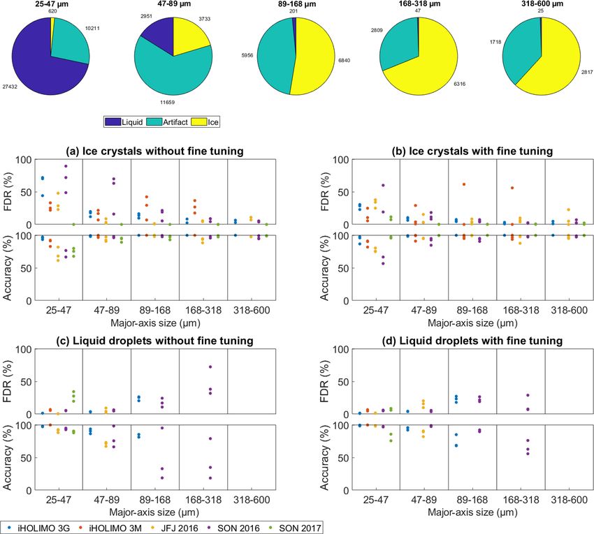
4.5 The CNN prediction performance over particle size bin. Results of size bins where datasets have less than 30
particles of the considered class were excluded due to insuf-
In order to assess the performance of the CNN with respect ficient statistical representativeness. This is mainly the case
to the particle size, the data were split into bins according to for droplets larger than 89 µm.
the major-axis size. Because the small particles outnumber The accuracy and FDR results without fine tuning being
the large particles, an exponentially increasing bin width was applied (Fig. 12a, c) show a strong variation in particle size.
chosen. The accuracies and FDRs of liquid droplets and ice In general, the prediction performance was worse for sizes
crystals for the pre-trained CNN on merged datasets without with a relatively and/or absolutely small amount of sam-
(Fig. 12a, c) and with fine tuning (Fig. 12b, d) are shown ples belonging to the considered class, e.g., for ice crystals
in Fig. 12 together with the class distribution of each size
Atmos. Meas. Tech., 13, 2219–2239, 2020 www.atmos-meas-tech.net/13/2219/2020/G. Touloupas et al.: A CNN for classifying cloud particles 2229
Figure 11. Box plots of the evaluation metrics of different classification algorithms trained on four merged datasets and tested on a fifth
dataset. Shown are the results of the decision tree, the SVM, the CNN and the fine-tuned CNN. The red lines in the boxes mark the medians,
while the box edges show the 25th and the 75th percentile respectively. The end of the whiskers are the most extreme data points, and the red
crosses mark outliers, which are defined as data points being more than 1.5 times the interquartile range away from the top or bottom of the
boxes.
smaller than 89 µm (median FDR: 20 %; median accuracy: Due to small numbers of samples, it is difficult to assess
93 %) and liquid droplets larger than 89 µm (median FDR: the performance of the CNN for liquid droplets larger than
25 %: median accuracy: 79 %). For the more common sizes, 89 µm. Only two datasets contained more than 30 particles
the values for ice crystals (median FDR: 5 %; median accu- for the larger three size bins, and the results show that the
racy: 99 %) as well as for liquid droplets (median FDR: 5 %; CNN performed poorly (median FDR: 25 %; median accu-
median accuracy: 92 %) are better. racy: 79 %) for liquid droplets in those size bins. However,
Independent of size, the FDR was generally larger for after fine tuning was applied the median FDR and accuracy
classes which are less frequent in the test dataset. This is improved to values of 22 % and 76 % respectively. We con-
expected as the misclassification of only a few percent of a clude that the CNN is not able to classify particles accurately
relatively prevalent class leads to a high FDR of a relatively in size bins where only a few data of the considered class are
small class. Since ice crystals are scarce compared to liquid available for training. However, the strong improvement af-
droplets in four datasets (see Table 1), their FDR is relatively ter fine tuning gives hope that this issue can be resolved after
high for ice compared to liquid (median FDR of ice: 12 %; collecting more data and retraining the network.
median FDR of liquid: 5 %), while the opposite holds true for
the SON 2017 dataset (median FDR of ice: 0 %; median FDR
of liquid: 28 %) where liquid droplets are underrepresented. 5 Discussion
In most cases, fine tuning led to an obvious improvement
in the accuracy and FDR (Fig. 12b, d). There was one outlier 5.1 Detecting mislabeled particles
for the FDR of ice crystals where one fine tuning run on the
dataset iHOLIMO 3M increased the FDR up to 20 %. It is The data used for training the various classification algo-
possible that an unusual or even mislabeled example of an rithms presented above were hand-labeled and therefore
ice crystal was in the randomly chosen fine tuning training prone to mislabeling. Mislabeling can happen either by cru-
sample which has a strong influence on the classification if cial mistakes or because the true class cannot be determined
there are not many other examples. Ignoring this one outlier, with certainty. Mislabeling is more crucial in rare classes
fine tuning of the merged CNN improved the results for the and/or size ranges.
accuracy as well as the FDR over all size bins; e.g., for the Mislabeled particles which have unusual diameters for
common sizes, the median FDR for ice crystals dropped from their class have a strong impact on the per-class accuracy or
5 % to 3 %, while the median accuracy for liquid droplets FDR in the corresponding size range and can, therefore, be
rose from 92 % to 98 %. For ice crystals smaller than 89 µm, detected as outliers (e.g., the orange dots in Fig. 12b). After
the median FDR dropped from 20 % to 11 %. re-evaluation of the label of those samples, the CNN should
be retrained. Uncertain cases should be excluded from the
training set to not bias the CNN. Correcting the mislabeled
www.atmos-meas-tech.net/13/2219/2020/ Atmos. Meas. Tech., 13, 2219–2239, 20202230 G. Touloupas et al.: A CNN for classifying cloud particles
Figure 12. Evaluation of the CNN trained on four merged datasets and tested on the remaining fifth dataset for different particle sizes. The
pie charts show the class distributions in the different size bins, while the graphs show the accuracy and FDR results for ice crystals and
liquid droplets before and after the fine tuning of three runs for the five datasets. Results of size bins where datasets have less than 30 particles
of the considered class are excluded due to insufficient statistical representativeness.
particles and excluding the uncertain particles have the po- 5.2 Comparison of the prediction performance of
tential to improve the prediction performance further. different classification algorithms
Training and testing the CNN, SVM and decision tree on the
same single dataset led to similar accuracies and low FDRs in
all cases (Fig. 9). When testing the same models on the other
four datasets (generalization), all metrics worsened with the
CNN showing slightly better results than the decision tree
and the SVM (Fig. 10). After merging four datasets and test-
ing on a fifth unseen dataset, the CNN surpassed the results of
the SVM and decision tree in almost every metric (Fig. 11).
Atmos. Meas. Tech., 13, 2219–2239, 2020 www.atmos-meas-tech.net/13/2219/2020/G. Touloupas et al.: A CNN for classifying cloud particles 2231
Table 2. The 15th, 50th and 85th percentiles of the DGTs for ice 5.4 Needed accuracy of cloud particle classification
crystals and liquid droplets of all sizes including all three runs (if regarding scientific questions
available) for each of the five datasets after fine tuning.
How accurate the phase discrimination, the particle number
Phase 15th, 50th and 85th percentile of the DGT ( %) or mass concentration has to be for a meaningful interpre-
Ice −3/4/10 tation of the data highly depends on the scientific question.
Liquid −1/1/6 For example, in a model study, Young et al. (2017) showed
that an overestimation of the ICNC (ice crystal number con-
centration) by only 17 % (2.43 L−1 instead of 2.07 L−1 ) led
Therefore, we conclude that the CNN outperforms the de- to cloud glaciation, while the MPC was persistent for about
cision tree and SVM in generalization tasks, which is espe- 24 h with a lower ICNC value, while very few ice crystals
cially pronounced when a high quantity of diverse data was (0.21 L−1 = −90 %) may lead to cloud breakup. In theoret-
used for training. ical calculation, Korolev and Isaac (2003) showed that the
Another important factor for the prediction performance glaciation time of an MPC with an ICNC of only 1 L−1 is
is the time it takes to do the predictions. This highly depends about 4 times as long as for 10 L−1 (+100 %) at a tempera-
on the dataset and the computational power of the computer. ture of −15 ◦ C. Comparing measurements with studies can
Classifying 10 000 particles takes about 15 s for the decision therefore already lead to wrong conclusions with classifica-
tree, about 30 s for the SVM and about 60 s for the CNN on a tion uncertainties of ±20 %.
local server. None of these timescales are comparable to the
time it takes to classify 10 000 particles by hand, which can
vary between a few hours and a few weeks depending on the 6 Conclusion and outlook
dataset.
In this work, we evaluated the performance of a CNN for the
5.3 Applying the CNN to new datasets
classification task of images of ice crystals, liquid droplets
We used the 15th and 85th percentile of the DGT of the and artifacts of sizes between 25 and 600 µm from holo-
three fine tuning runs for all five datasets as an estimate of graphic imagers. The important takeaways from our exper-
the lower and upper uncertainty. Thus, 70 % of the data is iments are summarized below.
included, which is similar to the definition of the standard
error. The 50th percentile is the median and indicates a sys- 6.1 CNN compared to other machine learning baselines
tematic bias. When considering the overall uncertainty, an
uncertainty of ±10 % for ice crystals and ±6 % for liquid When training and testing the network on data from a single
droplets is sufficient to include most of the spread observed dataset, the CNN achieved similar results compared to a de-
(see Table 2). For ice crystals smaller than 89 µm, the uncer- cision tree and an SVM. When training on a merged dataset
tainty has to be set higher or a systematic correction should and testing on an unseen dataset (generalization task), the
be applied, e.g., for ice crystals in the first size bin about 15 % CNN surpassed the results of the decision tree and the SVM
and for the second size bin about 5 % can be subtracted from in six out of seven metrics, with the median overall accuracy
the number of classified ice crystals with an uncertainty of being as high as 96.8 %. Using the CNN not only improved
±20 % for the first size bin and ±10 % for the other size bins the generalization ability but also requires less engineering
(see Table 3). effort, since it automatically extracts features from data, un-
According to Fig. 2.5 in Beck (2017), the automated clas- like decision trees and SVMs.
sification hitherto added about ±10 % up to about +60 % and
−40 % of uncertainty for particles smaller than 40 µm. Other 6.2 Fine tuning
sources of uncertainty like the manual classification con-
tribute with about ±5 % (see Fig. 3) to the size ranges con- After fine tuning the CNN trained on merged datasets with
sidered here. Therefore, the uncertainties using a fined-tuned only 256 samples from the target dataset, the median of the
CNN are of a similar magnitude to uncertainties from other overall accuracy improved from 96.8 % to 98.2 %. Similar
sources. Hence, the automated classification is no longer the improvements could be seen in all per-class accuracies and
main error source for the classification of small particles. FDRs. Labeling of 256 samples from the target dataset is a
However, the classification ability of the CNN cannot be as- very small amount of effort for improving the results consid-
sessed for droplets larger than 89 µm due to a lack of data in ering the millions of samples acquired during a typical field
that size range. excursion. However, the sample being used for fine tuning
has to be chosen carefully. All classes should be represented
in similar amounts. Otherwise, fine tuning can even worsen
the results.
www.atmos-meas-tech.net/13/2219/2020/ Atmos. Meas. Tech., 13, 2219–2239, 20202232 G. Touloupas et al.: A CNN for classifying cloud particles
Table 3. The 15th, 50th and 85th percentiles of the DGTs in percentage for ice crystals and liquid droplets for the different size bins including
all three runs (if available) for each of the five datasets after fine tuning.
Size ranges
25–47 µm 47–89 µm 89–168 µm 168–318 µm 318–600 µm
Ice −4/18/27 −3/4/12 −3/2/8 −4/1/6 −1/1/6
Liquid −2/1/5 −4/2/9 – – –
6.3 CNN performance over particle size 6.6 Outlook
Depending on the measurement parameter of interest (e.g., The use of the CNN to classify huge amounts of cloud par-
mass concentration), one might have to account for the vari- ticle data has a high potential to further constrain the phase
ation of the performance ability of the CNN over particles partitioning in MPCs. This will help to better understand the
size. Reanalysis should be done for liquid droplets larger than microphysical processes relevant for precipitation initiation
89 µm in diameter and ice crystals smaller than 89 µm but and the glaciation of clouds. To improve the prediction of
also for sizes where the number of ice crystals exceeds the the CNN especially in for the classes unusual size bins, more
number of liquid droplets by at least an order of magnitude data need to be collected and labeled, but also mislabeled
and vice versa. We hope to mitigate this issue by collecting particles should be relabeled or removed from the training
more data in these size ranges. dataset. Future plans also include adapting the CNN archi-
tecture presented in this paper to be capable of classifying
6.4 Input channels particles smaller than 25 µm and of discriminating between
different ice crystal habits. This will furthermore improve the
Using the phase images in addition to the amplitude images analysis of especially small cloud particles and may help to
improved the results, even though we were not able to ex- answer important research questions about primary and sec-
tract useful features of the phase images. This indicates that ondary ice production.
the CNN finds important features and might even exceed the
classification abilities of humans.
6.5 Usage for other imaging probes
The performance improvements seen after fine tuning was
applied to the CNN show the ability of the CNN to adapt
to different datasets. Therefore, we expect the CNN to also
work for other imaging probes when fine tuning is applied or
after retraining the CNN from scratch. However, the phase
channel has to be turned off, since common imaging probes
do not deliver phase images.
Atmos. Meas. Tech., 13, 2219–2239, 2020 www.atmos-meas-tech.net/13/2219/2020/G. Touloupas et al.: A CNN for classifying cloud particles 2233
Appendix A: Neural networks ing dataset X = {(x 1 , y1 ) , . . ., (x T , yT )}. Each training im-
age x t has a ground truth label yt associated to it. When x t is
The machine learning model used is a (deep) neural network used as the input to the neural network, the label f (x t ; W )=
which is used to discriminate between the three classes of ice yˆt is predicted. We can define a loss function L yt , yˆt that
crystal, liquid droplet and artifact. Deep neural networks are measures the performance of the network for each data sam-
part of a broader family of techniques commonly referred to ple, compared to the ground truth. A commonly used loss
as deep learning. Over the past few years, deep learning has function for multiclass classification is the softmax cross-
attracted a lot of attention in the machine learning commu- entropy method. The parameters of W are learned by min-
nity as well as in many other branches of science. One reason imizing the loss as follows:
for this success is the high performance they have achieved
on image classification (Krizhevsky et al., 2012). This suc- T
X
cess has to a large extent be attributed to their ability to learn W ∗ = arg min L (yt , f (x t ; W )) ,
W i=1
complex models while exhibiting good generalization prop-
erties. This means that these models are able to achieve good
where arg min stands for the argument of the minimum.
performance on new data that have not been seen while train-
This optimization problem is usually performed by using
ing the network.
a gradient-based optimization method like stochastic gradi-
A significant advantage of deep neural networks over more
ent descent (SGD). Such methods require the calculation of
traditional machine learning models such as SVMs or deci-
the local gradients for the loss and the parameters of the net-
sion trees is their ability to automatically learn useful data
work, which can be computed with the back-propagation al-
representations, thus eliminating the need for feature engi-
gorithm; see details in Goodfellow et al. (2016).
neering.
In this work, we use convolutional neural networks
(CNNs) (LeCun et al., 1989), a type of neural networks par- Appendix B: Pixel intensity distributions
ticularly suitable for processing data that have a grid-like
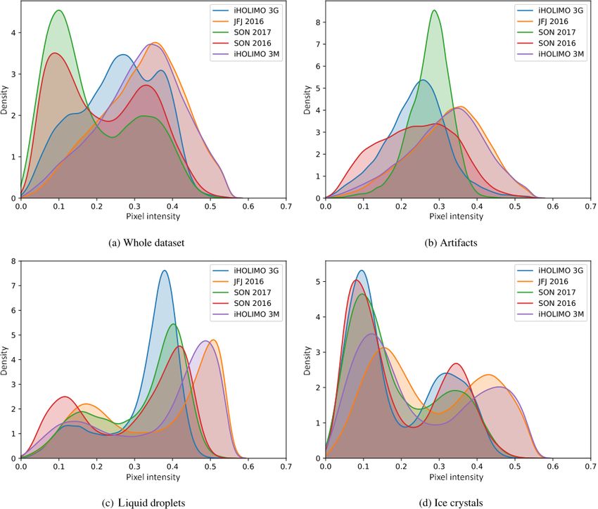
topology, such as images (grid of pixels). Here we give a An interesting aspect of the data is the pixel values for dif-
brief introduction to CNNs and provide more details in the ferent classes and different datasets. We use the amplitude of
other appendices. the original complex images and compute the KDE (kernel
density estimation) of the pixel intensity distribution for all
A1 Principle of a neural network the images of each class for every dataset. The bandwidths
of the kernels are computed using the rule in Scott (1979).
A neural network consists of an interconnected group of
The plots of the KDEs of the pixel intensity distributions are
nodes named neurons. A neuron n receives a d-dimensional
presented in Fig. B1.
vector x n = xn1 , . . ., xnd as an input and computes an output
We note that for all datasets the pixel intensity distribu-
variable on as
! tions of liquid droplets and ice crystals are bimodal. The peak
Xd at the lower intensity (darker) corresponds to the pixels of the
i i
o n = fn wn · xn , (A1) cloud particle shadow, whereas the peak at the higher inten-
i=1 sity (brighter) corresponds to the pixels of the background
where wn = wn1 , . . ., wnd describes the weight parameters
that is included in the extracted images. The pixel intensity
of the neuron n, and fn is a chosen activation function. The distribution for the artifacts has a single peak for all datasets.
weights w n are trainable, meaning that they can be updated This is due to the fact that most artifacts are noisy images.
while training the network. The purpose of the activation Another observation for all datasets is that the lower in-
function is to introduce nonlinearity into the otherwise linear tensity peak is lower than the higher intensity peak for liquid
model. Commonly used activation functions are the sigmoid, droplets, while the opposite is true for ice crystals. This is
the hyperbolic tangent and the rectified linear unit (ReLU; mainly due to the smaller size on average of liquid droplets
Nair and Hinton, 2010), defined as f (x) = max(0, x). compared to ice crystals. Since the background included in
The neurons of a network are organized in collections the extracted images is a fixed-size band of pixels around the
called layers. A neural network consists of connected lay- border of the particle, the smaller cloud particles will have a
ers, effectively computing a function f (x; W ) = ŷ, where x larger percentage of their image covered by background pix-
is the input image, W is the network parameters and ŷ is the els.
predicted label in a classification task setting. Aside from the aforementioned common characteristics,
there are also some dissimilarities in the pixel intensity dis-
A2 Training a neural network tributions for different datasets. First, the pixel intensities in
datasets iHOLIMO 3G, SON 2017 and SON 2016 fall for
The parameters W of the network are learned in a super- the larger part in the [0, 0.5] range, while those in datasets
vised manner by using labeled data samples from the train- JFJ 2016 and iHOLIMO 3M seem to be scaled to the [0, 0.6]
www.atmos-meas-tech.net/13/2219/2020/ Atmos. Meas. Tech., 13, 2219–2239, 2020You can also read