Computer Simulation of Neural Networks Using Spreadsheets: Dr. Anderson, Welcome Back

Computer Simulation of Neural Networks
 Using Spreadsheets: Dr. Anderson, Welcome Back

 Serhiy Semerikov1[0000-0003-0789-0272], Illia Teplytskyi1,
 Yuliia Yechkalo2[0000-0002-0164-8365], Oksana Markova2[0000-0002-5236-6640],
 Vladimir Soloviev1[0000-0002-4945-202X] and Arnold Kiv3
 1 Kryvyi Rih State Pedagogical University, 54, Gagarina Ave., Kryvyi Rih, 50086, Ukraine
 {semerikov, vnsoloviev2016}@gmail.com
 2 Kryvyi Rih National University, 11, Vitali Matusevich St., Kryvyi Rih, 50027, Ukraine

 uliaechk@gmail.com, markova@mathinfo.ccjournals.eu
 3 Ben-Gurion University of the Negev, Beer Sheba, Israel

 kiv@bgu.ac.il

 Abstract. The authors of the given article continue the series presented by the
 2018 paper “Computer Simulation of Neural Networks Using Spreadsheets: The
 Dawn of the Age of Camelot”. This time, they consider mathematical informatics
 as the basis of higher engineering education fundamentalization. Mathematical
 informatics deals with smart simulation, information security, long-term data
 storage and big data management, artificial intelligence systems, etc. The authors
 suggest studying basic principles of mathematical informatics by applying cloud-
 oriented means of various levels including those traditionally considered
 supplementary – spreadsheets. The article considers ways of building neural
 network models in cloud-oriented spreadsheets, Google Sheets. The model is
 based on the problem of classifying multi-dimensional data provided in “The Use
 of Multiple Measurements in Taxonomic Problems” by R. A. Fisher. Edgar
 Anderson’s role in collecting and preparing the data in the 1920s-1930s is
 discussed as well as some peculiarities of data selection. There are presented data
 on the method of multi-dimensional data presentation in the form of an ideograph
 developed by Anderson and considered one of the first efficient ways of data
 visualization.

 Keywords: Anderson’s Iris, cloud-based learning tools, computer simulation,
 mathematical informatics, neural networks, spreadsheets.

1 Introduction

The Fourth Industrial Revolution (Industry 4.0) actualized by the founder of the World
Economic Forum, Klaus Schwab, has become a system-related challenge for the
scientific community [15]. Industry 4.0 is primarily characterized by evolution and
convergence of nano-, bio-, information and cognitive technologies to enhance high
quality transformations in economic, social, cultural and humanitarian spheres.
Professionals dealing with development and introduction of the sixth technological

paradigm technologies determine to a great extent whether our country is able to ride
the wave of Industry 4.0 innovations. Therefore, extensive implementation of
information and communication technologies (ICT) is a top priority of Ukraine’s higher
education updating in order to form a professionally competent specialist able to ensure
the country’s innovative development.
 According to the Decree of the Cabinet of Ministers of Ukraine “Certain issues of
specifying medium-term priorities of the national-level innovative activity for 2017-
2021” (2016) [7], developing modern ICT and robotics, particularly cloud technologies,
computer training systems and technologies of mathematical informatics (intellectual
simulation, informational security, long-term data storage and “big data” management,
artificial intelligence systems) are nationally and socially important directions of the
innovative activity [10; 12].
 The Decree of the Cabinet of Ministers of Ukraine “Certain issues of specifying
medium-term priorities of the sectoral-level innovative activity for 2017-2021” (2017)
[8] specifies that these directions accompanied by smart web-technologies and cloud
computing make the basis for creating and defining themes for scientific researches and
technical (experimental) developments as well as for forming the state order of training
ICT specialists.

2 Literature Review and Problem Statement

Mathematical informatics is treated in two basic aspects:

1. as an area of

─ theoretical research (mathematical models and means are used to simulate and
 investigate information processes in various areas of human activity);
─ applied research (information systems and technologies are used to solve
 application-oriented problems).

2. as a subject which

─ studies basic models, methods and algorithms of solving the problems in
 intellectualization of information systems;
─ considers the issues of applying information models and information technologies
 of their study.

At the same time, the review in [9] ] has revealed that in spite of the significant role of
mathematical informatics in the computer sciences system, its models and methods are
not applied to computer engineering and software engineering at Ukraine’s higher
educational institutions in a consistent manner.
 In [11; 19; 23], the systematic training of students of technical universities (first of
all, IT-students) in mathematical informatics is substantiated and its leading methods
are determined. Introduction of mathematical informatics into university curricula is
theoretically based on fundamentalization of professional training as a means of
overcoming a gap between the training content and technological advance [24].

3

 Future training in mathematical informatics results in IT specialists’ ability to
modify available and elaborate new information technologies based on models and
methods of mathematical informatics in order to enhance the country’s innovative
development.
 In [10] the role of neural network simulation in the training content of the special
course “Foundations of Mathematical Informatics” is discussed. The course is
developed for students of technical universities (future IT-specialists) and aimed at
breaking a gap between theoretic computer science and its practical application to
software, system and computing engineering. CoCalc is justified as a training tool for
mathematical informatics in general and neural network modeling in particular. The
elements of CoCalc techniques for studying the topic “Neural network and pattern
recognition” within the special course “Foundations of Mathematical Informatics” are
shown.
 The authors of [16] distinguish basic approaches to solving the problem of network
computer simulation training in the spreadsheet environment, joint application of
spreadsheets and tools of neural network simulation, application of third-party add-ins
to spreadsheets, development of macros using the embedded languages of spreadsheets;
use of standard spreadsheet add-ins for non-linear optimization, creation of neural
networks in the spreadsheet environment without add-ins and macros.
 In [17; 18], there are opportunities for applying spreadsheets to introducing
essentials of machine learning [13] at secondary and higher school as well as some
elements of their application to solving problems of pattern classification.
 Thus, using spreadsheets as a tool for teaching basics of machine learning creates
conditions for early and simultaneously deeper mastering of corresponding models and
methods of mathematical informatics [2].

3 The Aim and Objectives of the Study

Therefore, the aim of the study is to develop certain components of the methods of using
electronic spreadsheets as a training tool for neural network simulation in the special
course “Foundations of Mathematical Informatics”.
 To accomplish the set goal, the following tasks are to be solved:

1. substantiation of chosen sets of data to develop a model;
2. development of a demonstration model of an artificial neural network using cloud-
 oriented spreadsheets.

4 Edgar Anderson and His “Fisher’s Iris Data Set” (1936)

Edgar Shannon Anderson (November 9, 1897 – June 18, 1969) was born in Forestville,
New York (Fig. 1). According to George Ledyard Stebbins, from an early age he
exhibited both superior intelligence and a great interest in plants, particularly in
cultivating them and watching them grow [20, p. 4].

Fig. 1. Edgar Anderson’s portrait and signature

He went to Michigan Agricultural College at the age of sixteen, just before his
seventeenth birthday, knowing already that he wanted to be a botanist. After completing
his degree, he accepted a graduate position at the Bussey Institution of Harvard
University. After leaving Harvard with his doctor’s degree in 1922, Anderson spent
nine years at the Missouri Botanical Garden, where he was a geneticist and Director of
the Henry Shaw School of Gardening; at the same time he was Assistant Professor, later
Associate Professor, of Botany at Washington University in St. Louis. During this
period, he developed the beginnings of his highly original and effective methods for
looking at and recording variation in plant populations, as well as his keen interest in
the needs and progress, both scientific and personal, of students in botany. His training
in genetics had given him habits of precision and mathematical accuracy in observing
and recording variation in natural populations that were entirely foreign to the
taxonomists of that period [20, p. 5].
 Through contacts with Jesse Greenman, Curator of the Garden Herbarium, he
became aware of the enormous complexity and extent of the variation present in any
large plant genus and of the need for understanding the origin of species as a major step
in evolution. On extensive field trips he began to realize that a great amount of genetic
variation exists within most natural populations of plants. This realization led him to
the conclusion that “if we are to learn anything about the ultimate nature of species we
must reduce the problem to the simplest terms and study a few easily recognized, well
differentiated species” [4, p. 243].
 He first selected Iris versicolor, the common blue flag, because he believed it to be
clearly defined, and it was common and easily observed. Initially, this appeared to be a
mistaken choice, since he soon found that Iris versicolor of the taxonomic manuals was
actually two species, which, after preliminary analysis, he could easily tell apart. He
then set himself the task of finding out, by a careful analysis of populations throughout

5

their geographic areas, how one of these species could have evolved from the other. He
recorded several morphological characters in more than 2,000 individuals belonging to
100 populations, data far more extensive than those that any botanist had yet obtained
on a single species.
 In order to enable these data to be easily visualized and compared, he constructed
the first of his highly original and extremely useful series of simplified diagrams or
ideographs (Fig. 2). By examining them, he reached the conclusion that the variation
within each of his two species was of another order from the differences between them;
no population of one species could be imagined as the beginning of a course of
evolution toward the other. He therefore concluded that speciation in this example was
not a continuation of the variation that gave rise to differences between populations of
one species, and started to look for other ways in which it could have taken place. The
current literature offered a possible explanation: hybridization followed by
chromosome doubling to produce a fertile, stable, true-breeding amphidiploid. To apply
this concept to Iris, he had to find a third species that would provide an alternate parent
for one of those studied. Going to the herbarium, he found it: an undescribed variety of
Iris setosa, native to Alaska.
 All of his data, including counts of chromosome numbers, agreed with the
hypothesis that Iris versicolor of northeastern North America had arisen as an
amphiploid, one parent being Iris virginica of the Mississippi Valley and the Southeast
Coast and the other being Iris setosa var. interior of the Yukon Valley, Alaska. This
was one of the earliest demonstrations that a plant species can evolve by hybridization
accompanied or followed by chromosome doubling. Moreover, it was the first one to
show that amphiploid or allopolyploid species could be used to support hypotheses
about previous distribution of species.
 Anderson’s research into Iris resulted in all the techniques in his later successful
work, namely:

1. careful examination of individual characteristics of plants growing in nature and
 progeny raised in the garden;
2. reduction of this variation to easily visualized, simple terms by means of scatter
 diagrams and ideographs;
3. extrapolation from a putative parental species and supposed hybrids to reconstruct
 the alternative parent;
4. development of testable hypotheses by synthesizing data from every possible source.

The Iris research was Anderson’s chief accomplishment during his first period at the
Missouri Botanical Garden. Toward the end of this period, in 1929-1930, he received a
National Research Fellowship to study in England. There he was guided chiefly by
geneticist J. B. S. Haldane, but he also studied cytology under C. D. Darlington and
statistics with R. A. Fisher. Haldane introduced him to the mutants of Primula sinensis,
which he analyzed in collaboration with Dorothea De Winton. Their joint research was
the first effort in plant material to relate pleiotropic gene action to growth processes.
 In 1931 Anderson went to Harvard, where he stayed until 1935, as an arborist at the
Arnold Arboretum. He returned to the Missouri Botanical Garden in 1935 and remained
there for the rest of his life. Returning to his study of the genus Iris, he and several

students analyzed a complex variation pattern of populations found in the Mississippi
delta region [3].
 Anderson integrated his new experience with past memories, popular accounts of his
methods of research, and his general philosophy of life in the book “Plants, Man and
Life” [2] published in 1952. It is a combination of scientific knowledge, folklore of
Latin American and other countries, and Anderson’s comments on early herbalists and
the habits of taxonomists and botany professors, plus a bit of philosophy. One of his
chief contributions to plant science, the pictorialized scatter diagram, is presented for
the first time in its final form in a chapter entitled, characteristically, “How to Measure
an Avocado” (Fig. 2).

 Fig. 2. Anderson’s pictorialized scatter diagram [2, p. 97]

In 1954 Anderson became Director of the Missouri Botanical Garden, but he found full-
time administration frustrating and in 1957 resigned and resumed his career of teaching
and research. During the 1960s he was plagued by illness, and his principal
contributions during that period were a steady flow of popular articles on trees, shrubs,
and other plants of the garden. He retired officially in 1967.
 Anderson’s article of 1936 [1] was his last work dedicated to the problem of Iris
origin and classification. In his introduction to the article, Anderson not only expressed
his gratitude to his English teachers, but also directly indicated that “Dr. Wright, Prof.
J. B. S. Haldane, and Dr. R. A. Fisher have greatly furthered the final analysis of the
data, though they are in no way responsible for the imperfections of the work or of its
presentation.” [1, p. 458].

7

 In 1936, Sir Ronald Aylmer Fisher published the article “The Use of Multiple
Measurements in Taxonomic Problems” indicating that “Table I shows measurements
of the flowers of fifty plants each of the two species Iris setosa and I. versicolor, found
growing together in the same colony and measured by Dr E. Anderson, to whom I am
indebted for the use of the data” [6, p. 179-180]. Fisher’s article contained only three
references two of which to Anderson’s works – that of 1935 [3] and that of [1] marked
with “(in the Press)”. In 1936, Fisher was not the member of the editorial board of
“Annals of the Missouri Botanical Garden”. The only way of his being aware of
Anderson’s article [1], was their personal correspondence.
 The set of data used by Fisher and collected by Anderson was introduced as “Iris
flower data set” (or “Iris data set” and “Iris data”). The phrase “Fisher’s Iris data set”
traditionally expresses Fisher’s role as the founder of linear discriminant analysis, but
not the authorship of the data set.
 Although Anderson never published these data, he described [3] how he collected
information on irises: “For some years I have been studying variation in irises but never
before have I had the good fortune to meet such quantities of material for observation.
On the simple assumption that if current theories are true, one should be able to find
evidence of continuing evolution in any group of plants, I have been going around the
world looking as sharply as possible at variation in irises. On any theory of evolution
the differences between individuals get somehow built up, in time, into the differences
between species. That is to say that by one process or another the differences which
exist between one plant of Iris versicolor and its neighbor are compounded into the
greater difference which distinguishes Iris versicolor from Iris setosa canadensis. It is
a convenient theory and if it is true, we should be able to find the beginnings of such a
compounding going on in our present day species. For that reason I have studied such
irises as I could get to see, in as great detail as possible, measuring iris standard after
iris standard and iris fall after iris fall, sitting squat-legged with record book and ruler
in mountain meadows, in cypress swamps, on lake beaches, and in English parks. The
result is still merely a ten year’s harvest of dry statistics, only partially winnowed and
just beginning to shape itself into generalizations which permit of summarization and
the building of a few new theories to test by other means.
 I have found no other opportunity quite like the field from De Verte to Trois Pistoles.
There for mile after mile one could gather irises at will and assemble for comparison
one hundred full-blown flowers of Iris versicolor and of Iris setosa canadensis, each
from a different plant, but all from the same pasture, and picked on the same day and
measured at the same time by the same person with the same apparatus. The result is,
to ordinary eyes, a few pages of singularly dry statistics, but to the biomathematician a
juicy morsel quite worth looking ten years to find.
 After which rhapsody on the beauty of variation it must immediately be emphasized
that Iris setosa canadensis varies but little in comparison with our other native blue
flags. Iris versicolor in any New England pastures may produce ground colors all the
way from mauve to blue and with hafts white or greenish or even sometimes quite a
bright yellow at the juncture with the blade. Iris setosa canadensis by contrast is
prevailingly uniform, its customary blue grey occasionally becoming a little lighter or
a little darker or even a little more towards the purple, and its tiny petals producing odd

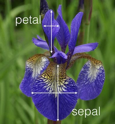
variants in form and pattern, but presenting on the whole only a fraction of the
variability of Iris versicolor from the same pasture.
 The reasons for this uniformity are not far to seek. Its lower chromosome number is
one, but a discussion of that and its bearings on the whole problem would be a treatise
in itself. More important probably is the fact that by geological and biological evidence,
Iris setosa canadensis is most certainly a remnant, a relict [sic] of what was before the
glacial period a species widely spread in northern North America.
 If we take a map and plot thereon all known occurrences of Iris setosa and Iris setosa
canadensis, we shall find the former growing over a large area at the northwest comer
of the continent, and the latter clustering in a fairly restricted circle about the Gulf of
St. Lawrence, while in the great intervening stretch of territory, none of these irises has
been collected. This is a characteristic distribution for plants which were almost
exterminated from eastern North America by the continental ice sheet, but while [sic]
managed to persist in the unglaciated areas about the Gulf of St. Lawrence from which
center they have later spread. In Alaska the species itself, Iris setosa, is apparently quite
as variable as our other American irises.”
 So, we should pay tribute to Edgar Anderson by naming this data set after him –
Anderson’s Iris data set.

5 Model development

As indicated in [10], the special course “Foundations of Mathematical Informatics”
final control of knowledge is a credit by the presentation of individual education and
research projects on the artificial neural networks built by using CoCalc. Students can
be offered to use cloud-based spreadsheets, Google Sheets, with the Solver additional
cloud-based component (add-in) which is similar to “Solver” in Excel Online.
 Let us consider the corresponding application method by taking a multi-dimensional
data set (Anderson’s Iris data set) to solve the pattern classification problem.
Anderson’s Iris is composed of data on 150 measurements of three Iris species (Fig. 3)
– Iris setosa, Iris virginica and Iris versicolor) – including 50 measurements for each
species.
 There were measured four features (Fig. 4): sepal length (SL), sepal width (SW),
petal length (PL), and petal width (PW).

 Fig. 3. Anderson’s Irises

9

 Fig. 4. Measurement features of Anderson’s Irises

To draw a grounded conclusion on the Iris type, we build a three-layered neural network
with the following architecture (Fig. 5):

─ the input layer is a four-dimensional arithmetical vector (x1, x2, x3, x4) the
 components of which are corresponding measured features of Anderson’s Irises
 (SL, SW, PL, PW) normalized according to the network activation function;
─ the hidden layer has dimension 9 (the minimal required number according to
 Kolmogorov–Arnold representation theorem) and is described by the vector
 (h1, h2, h3, h4, h5, h6, h7, h8, h9);
─ the output layer is a three-dimensional arithmetical vector (y1, y2, y3) the components
 of which are probabilities indicating the correspondence of the data set to one of the
 three Iris types.

The bias neuron equal to 1 (marked red in Fig. 5) is added to the neurons of the input
and hidden layers. The bias neurons are noted for not having synapses so they cannot
be located in the output layer.
 Let us first introduce Anderson’s Irises into spreadsheets with the following values
of cells: A1 is Iris Data, A2 is SL, B2 is SW, C2 is PL, D2 is PW, E2 is Species.
 The table cells A3:E152 include Anderson’s Irises (Fig. 6).
 We cannot input the data of the given set into the input layer as the value of the four
characteristics is beyond the range limits [0; 1]. The next step is normalization of
columns A, B, C and D to meet the given range and coding of Iris types from column
E.
 Each Iris type is coded by the three-dimensional arithmetical vector: for i-Iris (Iris
setosa is 1, Iris versicolor is 2, Iris virginica is 3) we set the i-th component in 1, and
the other ones – in 0. To do this, we introduce the following values into the cells: G1 is
encoding, G2 is setosa, H2 is versicolor, I2 is virginica, G3 is
=if($E3=G$2,1,0).
 Next, we copy the formula from the cell G3 to the range G3:I152 and obtain the
following model codes for the three Iris types: for Iris setosa – (1, 0, 0), for Iris virginica
– (0, 0, 1) and for Iris versicolor – (0, 1, 0).

4 features
 SL SW PL PW

 input layer

 x1 x2 x3 x4

 hidden layer

 h1 h2 h3 h4 h5 h6 h7 h8 h9

 output layer
 y1 y2 y3

 Anderson’s Iris type
Fig. 5. Architecture of the neural network to solve the problem of Anderson’s Iris classification

 Fig. 6. The fragment of the spreadsheet of Anderson’s Irises

 Each column is normalized separately. To perform this, we find minimum and
maximum values by introducing the following values: E154 is min, E155 is max, A154
is =min(A3:A152), A155 is =max(A3:A152).
 We apply the cells A154:A155 to the range B154:D155 and introduce the following
values into the cells: K1 is normalization, K2 is x1, L2 is x2, M2 is x3, N2 is x4, K3
is =(A3-A$154)/(A$155-A$154).
 The latter formula is a pplied to the range K3:N152. Its essence is explained by:
 value – min
 normalization = .
 max – min

 This approach results in the minimum value normalized to 0, while the maximum
one – to 1.

11

 According to the chosen architecture, we add the bias neuron to the four neurons of
the input layer by introducing its name (x5) into the cell O2 and its value (1) into the
range O3:O152. On this stage, the input layer is formed as x1, x2, x3, x4, x5.
 The next step includes transmission of a signal from the input layer to the hidden
one of the neural network. We denote the weight coefficient of the synapse connecting
the neuron xi (i = 1, 2, 3, 4, 5) of the input layer with the neuron hj (j = 1, 2, ..., 9) of the
hidden layer by wxhij, while the weight coefficient connecting the neuron hj of the hidden
layer with the neuron yk (k = 1, 2, 3) of the input layer is denoted by whyjk . In this case,
the force of the signal coming to the neuron hj of the hidden layer is determined as a
scalar product of signal values on the input signals and corresponding weight
coefficients. To determine a signal going further to the output layer, we apply the
logistic function of activation f(S) = 1/(1+e–S), where S is a scalar product. The formulae
for determining the signals on the hidden and output layers will look like:
 4+1 9+1
 ℎ 
 ℎ = (∑ ℎ ) , = (∑ ).
 =1 =1

Accordingly, two matrices should be created. The matrix wxh of 59 contains weight
coefficients connecting five neurons of the input layer (the first four contain normalized
characteristics of Anderson’s Irises, while the fifth one is the bias neuron) with the
neurons of the hidden layer. The matrix why of 103 contains weight coefficients
connecting ten neurons of the hidden layer (nine of which are calculated and the tenth
one is the bias neuron) with the neurons of the output layer. For the “untaught” neural
network, initial values of the weight coefficients can be set either randomly or left
undetermined or equal to zero. To realize the latter, we fill the cells with the following
values: R1 is wxh, Q2 is input/hidden, R2 is 1, S2 is =R2+1, Q3 is 1, Q4 is =Q3+1, R3
is 0, R9 is why, Q10 is hidden/output, R10 is 1, S10 is =R10+1, Q11 is 1, Q12 is
=Q11+1, R11 is 0.
 To create the matrices, we should copy the cells R3 into the range R3:Z7, R11 – into
R11:T20, S2 – into T2:Z2, Q4 – into Q5:Q7, S10 – into T10, Q12 – into Q13:Q20
(Fig. 7).
 To calculate the scalar product of the vector row of the input layer values by the
matrix vector-column of the weight coefficients why, we should apply the matrix
multiplication function: AB1 is calculate the hidden layer, AB2 is h1, AC2 is
h2, AD2 is h3, AE2 is h4, AF2 is h5, AG2 is h6, AH2 is h7, AI2 is h8, AJ2 is h9, AK2 is
h10, AB3 is =1/(1+exp(-mmult($K3:$O3,R$3:R$7))), AK3 is 1.
 Next, we copy the cell AK3 into the range AK4:AK152, while AB3 – into
AB3:AJ152.
 Considering the fact that all the matrix elements of the weight coefficients wxh equal
to zero, after duplicating the formulae, the calculated elements of the hidden layer will
be equal to 0.5.
 In the same way, we calculate the output layer elements: AM1 is calculate the
output layer, AM2 is y1, AN2 is y2, AO2 is y3, AM3 is
=1/(1+exp(-mmult($AB3:$AK3,R$11:R$20))).

Fig. 7. The fragment of the spreadsheet after coding and normalization of the output data and
 creation of the matrices of the weight coefficients

 Next, we copy the cell AM3 to the range AM3:AO152 (Fig. 8).

Fig. 8. The fragment of the spreadsheet of calculating the hidden and output layers with initial
 values of the weight coefficients

Neural network training is performed by varying weight coefficients so that with each
training step the difference between the calculated values of the output layer and the
desired (reference ones) reduces. To solve the problem, the three-dimensional vectors
resulted from coding of the three Iris types are reference.
 To find the difference between the calculated and the reference output vectors we
apply the Euclidean distance: AQ2 is distance, AR2 is sum of distances, AQ3 is
=sqrt((AM3-G3)^2+(AN3-H3)^2+(AO3-I3)^2), AR3 is =sum(AQ3:AQ152).
 Next, we copy the cell AQ3 to the range AQ4:AQ152. The cell AR3 contains general
deviation of the calculated output vectors from the reference ones.
 Under this approach, the neural network training can be treated as an optimization
problem in which the target function (the sum of distances in the cell AR3) will be
minimized by varying the matrix weight coefficients wxh (the range R3:Z7) and why (the
range R11:T20). To solve this problem, application of cloud-oriented spreadsheets
(Google Sheets) is not enough and it is necessary to install an additional cloud-oriented
component (add-in) Solver.
 Adjustment of the add-in Solver to solve the set goal: the target function (Set
Objective) is minimized (To: Min) by changing the values (By Changing) of the matrix

13

weight coefficients in the range (Subject To) from –10 tо +10 by one of the optimization
methods (Solving Method).
 To reduce the total distances, the actions with Solver can be done repeatedly as it is
expedient to experiment with combination of various optimization methods by
changing the variation limits of the weight coefficients. It is not necessary to try to
reduce the value of the total distances to zero as this can be a greater (quite smaller)
value (Fig. 9).

 Fig. 9. Optimization results

On the assumption of the chosen coding method, the output vector actually contains
three probabilities: yi denotes the probability of the given sample being the i-type Iris,
where i = 1 for Iris setosa, 2 for Iris versicolor and 3 for Iris virginica. Then, to find out
which Iris type describes the input vector (SL, SW, PL, PW), the most probable
component should be determined.
 To do this, we fill the cells in the following way: AT2 is Calculated Iris
species, AT3 is =if(max(AM3:AO3)=AM3,$G$2,if(max(AM3:AO3)=AN3,$H$2,
$I$2)), AU3 is =if(AT3=E3,"right!","wrong").
 Next, the range AT3:AU3 is copied to the range AT4:AU152.
 The obtained result enables us to visualize pattern recognition simulated in
spreadsheets. The built model will be considered relevant in all 150 cases, the column
AU contains the value "right!".
 To check the limits of the built model application, we try to input the vector not
coinciding with any reference input vector. For this, we copy the table row 152 to 158
and delete the content of the cells E158:I158, AQ158, AU158. We introduce averaged
values borrowed from the description of Iris versicolor in the article by Anderson [11,
p. 463]: 5.50, 2.75, 3.50 and 1.25. The reference values x1 = 0.3333, x2 = 0.3125,
x3 = 0.4237, x1 = 0.4792 are conveyed to the input layer, while on the hidden layer there
are calculated h1 = 0.0206, h2 = 0.4419, h3 = 0.0005, h4 = 0.0001, h5 = 0.9993,
h6 = 0.9993, h7 = 0.0001, h8 = 0.0288, h9 = 0.9991 and the values of the output layer
y1 = 0.0000, y2 = 1.0000, y3 = 0.0000. As the maximum value of the output layer 1.0000
corresponds to the other Iris type, we can conclude that Iris versicolor is identified.

6 Conclusions

1. Edgar Anderson appeared to be not a simple botanist whose data were the basis for
 Fisher’s known method. Anderson’s Irises resulted from his long experience of
 working out relevant models to describe changes in specific populations by means
 of a limited number of characteristics. Yet, Anderson had also coped with the
 opposite problem of building simple multi-dimensional data interpretation 40 years
 before Chernoff faces appeared [5].
2. The described methods of applying cloud-oriented spreadsheets as a tools for
 training mathematical informatics can enable solution of all basic problems of neural
 network simulation. The only limitation is not so much the volume of a spreadsheet
 as the memory space and the speed of the device processing it. In the special course
 projects if the limitation is overcome, this becomes a stimulus for replacing the
 simulation environment by a more relevant one [22].
3. The further research is the Dawn of the Age of Camelot: from Donald Hebb to
 Seymour Papert [17].

References
1. Anderson E.: The Species Problem in Iris. Annals of the Missouri Botanical Garden. 23(3),
 457–469+471–483+485–501+503–509 (1936). doi:10.2307/2394164.
2. Anderson, E.: Plants, Man and Life. University of California Press, Boston (1952)
3. Anderson, E.: The irises of the Gaspé Peninsula. Bulletin of the American Iris Society. 59,
 2–5 (1935)
4. Anderson, E.: The Problem of Species in the Northern Blue Flags, Iris versicolor L. and Iris
 virginica L. Annals of the Missouri Botanical Garden. 15(3), 241–332 (1928).
 doi:10.2307/2394087
5. Chernoff, H.: The Use of Faces to Represent Points in K-Dimensional Space Graphically.
 Journal of the American Statistical Association. 68(342), 361–368 (1973)
6. Fisher, R.A.: The Use of Multiple Measurements in Taxonomic Problems. Annals of
 Eugenics. 7(2), 179–188 (1936). doi:10.1111/j.1469-1809.1936.tb02137.x
7. Kabinet Ministriv Ukrainy: Deiaki pytannia vyznachennia serednostrokovykh
 priorytetnykh napriamiv innovatsiinoi diialnosti zahalnoderzhavnoho rivnia na 2017-2021
 roky (Certain issues of specifying medium-term priorities of the national-level innovative
 activity for 2017-2021). Zakonodavstvo Ukrainy.
 https://zakon.rada.gov.ua/laws/show/1056-2016-%D0%BF (2016). Accessed 21 Mar 2019
8. Kabinet Ministriv Ukrainy: Deiaki pytannia vyznachennia serednostrokovykh
 priorytetnykh napriamiv innovatsiinoi diialnosti haluzevoho rivnia na 2017-2021 roky
 (Certain issues of specifying medium-term priorities of the sectoral-level innovative
 activity for 2017-2021). Zakonodavstvo Ukrainy.
 https://zakon.rada.gov.ua/laws/show/980-2017-%D0%BF (2017). Accessed 21 Mar 2019
9. Kiv, A.E., Semerikov, S.O., Soloviev, V.N., Striuk, A.M.: First student workshop on
 computer science & software engineering. In: Kiv, A.E., Semerikov, S.O., Soloviev, V.N.,
 Striuk, A.M. (eds.) Proceedings of the 1st Student Workshop on Computer Science &
 Software Engineering (CS&SE@SW 2018), Kryvyi Rih, Ukraine, November 30, 2018.

15

 CEUR Workshop Proceedings. 2292, 1–10. http://ceur-ws.org/Vol-2292/paper00.pdf
 (2018). Accessed 31 Dec 2018
10. Markova, O., Semerikov, S., Popel, M.: CoCalc as a Learning Tool for Neural Network
 Simulation in the Special Course “Foundations of Mathematic Informatics”. In: Ermolayev,
 V., Suárez-Figueroa, M.C., Yakovyna, V., Kharchenko, V., Kobets, V., Kravtsov, H.,
 Peschanenko, V., Prytula, Ya., Nikitchenko, M., Spivakovsky A. (eds.) Proceedings of the
 14th International Conference on ICT in Education, Research and Industrial Applications.
 Integration, Harmonization and Knowledge Transfer (ICTERI, 2018), Kyiv, Ukraine, 14-
 17 May 2018, vol. II: Workshops. CEUR Workshop Proceedings. 2104, 338–403.
 http://ceur-ws.org/Vol-2104/paper_204.pdf (2018). Accessed 30 Nov 2018
11. Markova, O.M., Semerikov, S.O., Striuk, A.M.: The cloud technologies of learning: origin.
 Information Technologies and Learning Tools. 46(2), 29-44 (2015).
 doi:10.33407/itlt.v46i2.1234
12. Markova, O.M.: The tools of cloud technology for learning of fundamentals of
 mathematical informatics for students of technical universities. In: Semerikov, S.O.,
 Shyshkina, M.P. (eds.) Proceedings of the 5th Workshop on Cloud Technologies in
 Education (CTE 2017), Kryvyi Rih, Ukraine, April 28, 2017. CEUR Workshop
 Proceedings. 2168, 27–33. http://ceur-ws.org/Vol-2168/paper5.pdf (2018). Accessed 15
 Sep 2018
13. Mitchell, T.M.: Key Ideas in Machine Learning.
 http://www.cs.cmu.edu/%7Etom/mlbook/keyIdeas.pdf (2017). Accessed 28 Jan 2019
14. Modlo, Ye.O., Semerikov, S.O.: Xcos on Web as a promising learning tool for Bachelor’s
 of Electromechanics modeling of technical objects. In: Semerikov, S.O., Shyshkina, M.P.
 (eds.) Proceedings of the 5th Workshop on Cloud Technologies in Education (CTE 2017),
 Kryvyi Rih, Ukraine, April 28, 2017. CEUR Workshop Proceedings. 2168, 34–41.
 http://ceur-ws.org/Vol-2168/paper6.pdf (2018). Accessed 15 Sep 2018
15. Schwab, K., Davis, N.: Shaping the Fourth Industrial Revolution. Portfolio Penguin,
 London (2018)
16. Semerikov, S.O., Teplytskyi, I.O., Yechkalo, Yu.V., Kiv, A.E.: Computer Simulation of
 Neural Networks Using Spreadsheets: The Dawn of the Age of Camelot. In: Kiv, A.E.,
 Soloviev, V.N. (eds.) Proceedings of the 1st International Workshop on Augmented Reality
 in Education (AREdu 2018), Kryvyi Rih, Ukraine, October 2, 2018. CEUR Workshop
 Proceedings. 2257, 122–147. http://ceur-ws.org/Vol-2257/paper14.pdf. Accessed 21 Mar
 2019
17. Semerikov, S.O., Teplytskyi, I.O.: Metodyka uvedennia osnov Machine learning u
 shkilnomu kursi informatyky (Methods of introducing the basics of Machine learning in the
 school course of informatics). In: Problems of informatization of the educational process in
 institutions of general secondary and higher education, Ukrainian scientific and practical
 conference, Kyiv, October 09, 2018, pp. 18–20. Vyd-vo NPU imeni M. P. Drahomanova,
 Kyiv (2018)
18. Semerikov, S.O.: Zastosuvannia metodiv mashynnoho navchannia u navchanni
 modeliuvannia maibutnikh uchyteliv khimii (The use of machine learning methods in
 teaching modeling future chemistry teachers). In: Starova, T.V. (ed.) Technologies of
 teaching chemistry at school and university, Ukrainian Scientific and Practical Internet
 Conference, Kryvyi Rih, November 2018, pp. 10–19. KDPU, Kryvyi Rih (2018)
19. Shokaliuk, S.V., Markova, O.M., Semerikov, S.O.: SageMathCloud yak zasib khmarnykh
 tekhnolohii kompiuterno-oriientovanoho navchannia matematychnykh ta informatychnykh
 dystsyplin (SageMathCloud as the Learning Tool Cloud Technologies of the Computer-

Based Studying Mathematics and Informatics Disciplines). In: Soloviov, V.M. (ed.)
 Modeling in Education: State. Problems. Prospects, pp. 130-142. Brama, Cherkasy (2017)
20. Stebbins, G.L.: Edgar Anderson 1897-1969. National Academy of Sciences, Washington
 (1978)
21. Syrovatskyi, O.V., Semerikov, S.O., Modlo, Ye.O., Yechkalo, Yu.V., Zelinska, S.O.:
 Augmented reality software design for educational purposes. In: Kiv, A.E., Semerikov,
 S.O., Soloviev, V.N., Striuk, A.M. (eds.) Proceedings of the 1st Student Workshop on
 Computer Science & Software Engineering (CS&SE@SW 2018), Kryvyi Rih, Ukraine,
 November 30, 2018. CEUR Workshop Proceedings. 2292, 193–225. http://ceur-
 ws.org/Vol-2292/paper20.pdf (2018). Accessed 31 Dec 2018
22. Teplytskyi, I.O., Teplytskyi, O.I., Humeniuk, A.P.: Seredovyshcha modeliuvannia: vid
 zaminy do intehratsii (Modeling environments: from replacement to integration). New
 computer technology. 6, 67–68 (2008)
23. Turavinina, O.M., Semerikov, S.O.: Zmist navchannia osnov matematychnoi informatyky
 studentiv tekhnichnykh universytetiv (Contents of the learning of the foundations of
 mathematical informatics of students of technical universities). In: Proceedings of the
 International scientific and methodical conference on Development of intellectual abilities
 and creative abilities of students and students in the process of teaching disciplines of the
 natural sciences and mathematics cycle, Sumy State Pedagogical University named after
 A. S. Makarenko, Sumy, 6-7 December 2012, pp. 142–145. Vyd-vo SumDPU im.
 A. S. Makarenka, Sumy (2012)
24. Turavinina, O.M.: Matematychna informatyka u systemi fundamentalizatsii navchannia
 studentiv tekhnichnykh universytetiv (Mathematical informatics in the system
 fundamentalization learning the students of technical universities). Zbirnyk naukovykh
 prats Kamianets-Podilskoho natsionalnoho universytetu. Seriia pedahohichna. 18, 189-191
 (2012)