On the estimation of vertical air velocity and detection of atmospheric turbulence from the ascent rate of balloon soundings
←
→
Page content transcription
If your browser does not render page correctly, please read the page content below
Atmos. Meas. Tech., 13, 1989–1999, 2020
https://doi.org/10.5194/amt-13-1989-2020
© Author(s) 2020. This work is distributed under
the Creative Commons Attribution 4.0 License.

On the estimation of vertical air velocity and detection of
atmospheric turbulence from the ascent rate of balloon soundings
Hubert Luce1 and Hiroyuki Hashiguchi2
1 Mediterranean  Institute of Oceanography, MIO UM 110, IRD, Univ Toulon, Aix Marseille Univ.,
CNRS/INSU, La Garde, 83041, France
2 Research Institute for Sustainable Humanosphere, Kyoto University, Kyoto, 611-0011, Japan

Correspondence: Hubert Luce (luce@univ-tln.fr)

Received: 25 September 2019 – Discussion started: 30 September 2019
Revised: 16 December 2019 – Accepted: 4 February 2020 – Published: 21 April 2020

Abstract. Vertical ascent rate VB of meteorological bal-          fluctuations can be made if localized turbulence effects are
loons is sometimes used for retrieving vertical air veloc-        ignored.
ity W , an important parameter for meteorological applica-
tions, but at the cost of crude hypotheses on atmospheric
turbulence and without the possibility of formally validat-
ing the models from concurrent measurements. From simul-          1   Introduction
taneous radar and unmanned aerial vehicle (UAV) measure-
ments of turbulent kinetic energy dissipation rates ε, we show    The vertical ascent rates VB of meteorological balloons are
that VB can be strongly affected by turbulence, even above        mainly the combination of the free lift and fluctuations due
the convective boundary layer. For “weak” turbulence (here        to vertical air velocities and variations in atmospheric tur-
ε.10−4 m2 s−3 ), the fluctuations of VB were found to be          bulence drag effects. Despite balloons’ frequent use all over
fully consistent with W fluctuations measured by middle and       the world, few studies have tried to extract information from
upper atmosphere (MU) radar, indicating that an estimate of       VB . Most of these studies have focused on the estimation
W can indeed be retrieved from VB if the free balloon lift        of the vertical air velocity because this parameter is very
is determined. In contrast, stronger turbulence intensity sys-    important for many meteorological applications (e.g., Wang
tematically implies an increase in VB , not associated with       et al., 2009) and for the characterization of internal gravity
an increase in W according to radar data, very likely due to      waves (e.g., McHugh et al., 2008). Evidence of internal grav-
the decrease in the turbulence drag coefficient of the balloon.   ity wave fluctuations in balloon ascent rates was reported by
From the statistical analysis of data gathered from 376 bal-      Corby (1957), Reid (1972), and Lalas and Einaudi (1980).
loons launched every 3 h at Bengkulu (Indonesia), positive        Shutts et al. (1988) and Reeder et al. (1999) described large
VB disturbances, mainly observed in the troposphere, were         amplitude gravity waves in the stratosphere from the analy-
found to be clearly associated with Ri.0.25, usually indica-      ses of VB .
tive of turbulence, confirming the case studies. The analy-          However, the models or methods used for retrieving ver-
sis also revealed the superimposition of additional positive      tical air velocity from balloon ascent rates are often based
and negative disturbances for Ri.0.25 likely due to Kelvin–       on crude assumptions about atmospheric turbulence: it is ei-
Helmholtz waves and large-scale billows. From this experi-        ther considered more or less uniform or neglected above the
mental evidence, we conclude that the ascent rate of meteo-       planetary boundary layer. Johansson and Bergström (2005)
rological balloons, with the current performance of radioson-     estimated the height of boundary layers from VB consider-
des in terms of altitude accuracy, can potentially be used for    ing that VB is mainly affected by turbulence in convective
the detection of turbulence. The presence of turbulence com-      boundary layers. In fact, the free stratified atmosphere usu-
plicates the estimation of W , and misinterpretations of VB       ally reveals a “sheet and layer” structure (e.g., Fritts et al.,
                                                                  2003) consisting of more or less deep layers of turbulence

Published by Copernicus Publications on behalf of the European Geosciences Union.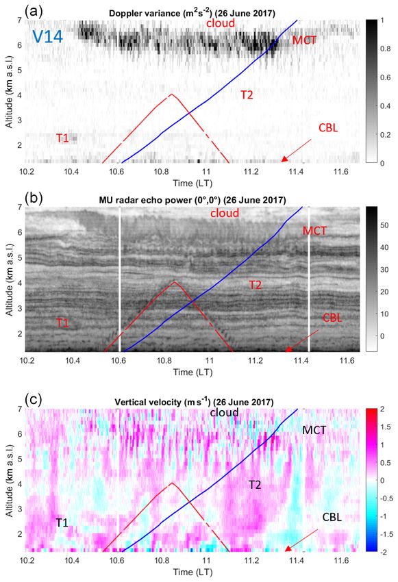
1990                                                   H. Luce and H. Hashiguchi: On the estimation of vertical air velocity

(a few hundred meters) separated by quieter and generally          of air motion is accurately taken into account. This alterna-
statically stable regions. In such conditions, turbulence inten-   tive purpose seems to be more achievable than retrieving W ,
sity, often quantified by turbulence kinetic energy dissipation    except at stratospheric heights and during very calm tropo-
rates, can vary over several orders of magnitude with height       spheric conditions, as shown by earlier studies, and likely
and can reach levels similar to those met in the convective        during deep convective storms during which strong vertical
atmospheric boundary layers (e.g., Luce et al., 2019).             motions are expected.
   In addition, most studies did not validate their estima-           The effects of turbulence on the balloon ascent rate can be
tions from concurrent measurements of vertical air veloc-          understood considering that this parameter in still air is given
ities, making their models and hypotheses uncertain (e.g.,         by (Gallice et al., 2011)
McHugh et al., 2008; Gallice et al., 2011). Gallice et
al. (2011) proposed a model to describe balloon ascent rates              s
                                                                              8Rg       3mtot
in the presence of free-stream turbulence. Even if the vari-       Vz =             1−             ,                              (1)
ations in the drag coefficient with altitude were taken into                  3cD      4π ρa R 3
account, their expression of the drag coefficient was based
on a mean turbulent state, and, thus, the model did not con-       where R is the radius of the volume-equivalent sphere, g is
sider the possibility of localized layers of turbulence, as ac-    the acceleration of gravity, ρa is the air density, and mtot is the
knowledged by the authors. Wang et al. (2009) retrieved ver-       total mass of the balloon–radiosonde system. The drag coef-
tical air velocity from radiosondes and dropsondes assum-          ficient, cD , depends on the Reynolds number associated with
ing that turbulence has a negligible effect above the convec-      the balloon Re = ρa Vz R/µ, where µ is the dynamic viscos-
tive boundary layer such that the drag coefficient was nearly      ity of air. The variation in cD with Re for a perfect sphere in
constant. Comparisons with wind profiler data (their Fig. 7)       the absence of atmospheric turbulence and for various values
showed poor agreement. Most profiles revealed oscillations,        of turbulence intensity Tu , defined as the ratio of the standard
indicative of gravity waves. McHugh et al. (2008) noted large      deviation of the incident air velocity fluctuations to the mean
(always positive) variations in balloon ascent rate around         incident air velocity (e.g., Son et al., 2010), is shown in Fig. 1
the tropopause over Hawaii and interpreted these localized         of Gallice et al. (2011). cD suddenly decreases by a factor 4
peaks as strong increases in W due to mountain waves around        to 5 above a critical value of Re (called drag crisis) so that
their critical levels. Independent measurements could not val-     Vz can increase by a factor 2 or more. In the presence of
idate this interpretation, and possible turbulence effects were    atmospheric turbulence, the drag crisis is displaced toward
not considered when interpreting observations. Houchi et           lower values of Re so that cD can be reduced when cross-
al. (2015) used a model similar to Wang et al.’s (2009) model      ing a turbulent layer. Recently, Söder et al. (2019) compared
for statistical estimates of the vertical air velocity. The au-    a profile of Re with a profile of balloon ascent rate (their
thors assumed that the balloon ascent rate is the sum of the       Fig. A1) and clearly showed the existence of a drag crisis
ascent rate in still air and vertical air velocity.                about Re ∼ 4 × 10⁵ in close agreement with the theoretical
   Modeling the ascent of balloons is not an easy task, espe-      expectation for a sphere (Fig. 1 of Gallice et al., 2011). Gal-
cially if the free-stream turbulence effects are not correctly     lice et al. (2011) proposed another (smoother) model from
taken into account. In the present work, we study the ef-          experimental data with a more realistic shape of balloons and
fects of turbulence on VB from experimental data. For this         with more complete consideration of the heat imbalance be-
purpose, vertical profiles of VB are compared with profiles        tween balloon and atmosphere. Their drag curve presented
of turbulence kinetic energy (TKE) dissipation rate ε esti-        qualitative similarities with the curves by Son et al. (2010)
mated from unmanned aerial vehicle (UAV) data and from             for a mean turbulent state of the atmosphere at Tu = 6 % and
46.5 MHz middle and upper atmosphere (MU) radar data.              Tu = 8 %. The fact that the model proposed by Gallice et al.
These data were gathered during Shigaraki UAV-Radar Ex-            does not consider the variability of turbulence with height is
periment (ShUREX) campaigns at the Shigaraki MU obser-             likely a weak point because turbulence is generally confined
vatory (Kantha et al., 2017). In addition, the MU radar pro-       to layers of variable depth in the troposphere and the strato-
vided coincident estimates of vertical air velocities so that      sphere.
quantitative comparisons with VB could be made. We found              In Sect. 2, we briefly describe the methods used for retriev-
that a balloon is likely a good “W sensor” in the case of light    ing the atmospheric parameters analyzed in the present study.
turbulence only: under the conditions of our experiment, VB        In Sect. 3, we show comparison results between VB , vertical
is affected by turbulence and thus cannot be used for esti-        velocity measured by MU radar, energy dissipation rate, and
mating W when ε&10−4 m2 s−3 (1 mW kg−1 ). Therefore, a             Richardson number profiles from three case studies selected
balloon is potentially more a “turbulence sensor” than a “W        from ShUREX2017. These comparisons clearly indicate that
sensor”, and very large errors in W can arise if the presence      turbulence effects dominate the balloon ascent rate. The re-
of free-stream turbulence is not properly considered. Alter-       sults of a statistical analysis from 376 balloons and based
nately, statistics on the occurrence of atmospheric turbulence     on the intimate relationship between turbulence and Richard-
could be made from balloon ascent rates if the contribution        son number Ri are shown in Sect. 4. They confirm that VB

Atmos. Meas. Tech., 13, 1989–1999, 2020                                                www.atmos-meas-tech.net/13/1989/2020/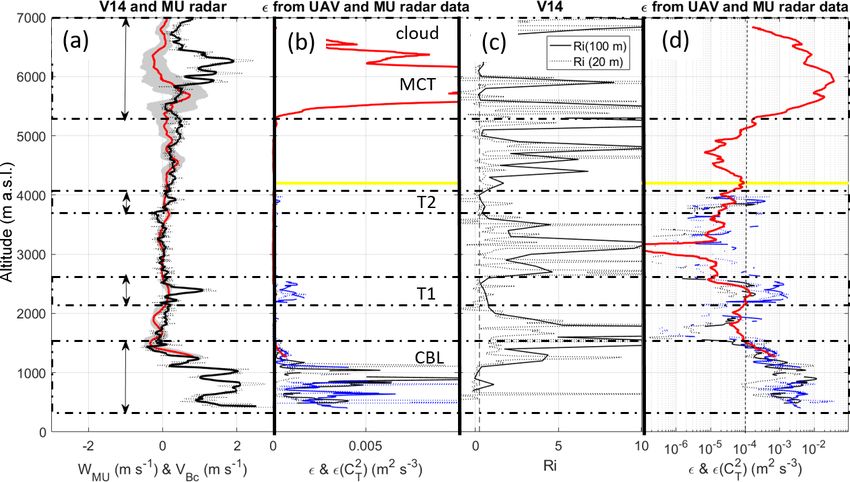
H. Luce and H. Hashiguchi: On the estimation of vertical air velocity                                                            1991

                                                                       measurements. An indirect estimate is deduced from the tem-
                                                                       perature structure function parameter CT2 calculated from 1D
                                                                       temperature spectra. Similar levels of ε and ε(CT2 ) give cre-
                                                                       dence to the results since the two estimates are independent.
                                                                       In addition, consecutive profiles can be obtained during UAV
                                                                       ascents and descents, depending on the configuration of the
                                                                       flights. Therefore, both vertical profiles of ε and ε(CT2 ) dur-
                                                                       ing ascents and descents will be shown when available.
                                                                          The TKE dissipation rate can also be estimated from MU
Figure 1. Horizontal trajectories of the meteorological balloons V6,   radar data using the variance σ 2 of Doppler spectrum peaks
V14 and V16. Each asterisk shows altitudes of 1 km, 2 km, etc., up     produced by turbulence. It is based on an empirical model
to 7 km. The position (0, 0) corresponds to the location of the Shi-   proposed by Luce et al. (2018) and validated from compar-
garaki MU Observatory. The circular patterns of the UAV trajecto-      isons with UAV-derived ε. The expression of the model is
ries are also shown.                                                   ε (MU) = σ 3 /Lout where Lout ∼ 60 m. In the present work,
                                                                       an estimate of ε (MU) at a given altitude z is obtained from
                                                                       an average of the values of σ 2 over a centered-in-time 2 min
is dominated by turbulence effects when Ri.0.25. Finally,              window (about 30 values since radar profiles were obtained
conclusions of this work are given in Sect. 5.                         every ∼ 4 s) around the time that the altitude z was reached
                                                                       by the radiosonde (see also Fig. 1 of Luce et al., 2018, for a
                                                                       schematic). This procedure should ensure that the estimates
2     Methods
                                                                       of ε are representative of those met by the balloons, assum-
2.1    Estimation of VB                                                ing horizontal homogeneity over a distance at least equal to
                                                                       the horizontal distance separating the balloons and the radar
Rubber balloons 200 g in weight and manufactured by TO-                (up to ∼ 30 km; see Sect. 3). The horizontal distance between
TEX were equipped with Vaisala RS92SGPD radiosondes                    UAV and balloon measurements did not exceed ∼ 10 km up
for pressure, temperature, relative humidity and horizontal            to the altitude of ∼ 4.0 km. Considering that all the turbulent
wind measurements during ShUREX campaigns. Their as-                   events analyzed in the present study persisted for more than
cent rate VB was calculated from 1z/1t where z is the GPS              1 h and were likely associated with meso- or synoptic-scale
altitude of the radiosondes and 1t = 2 s. A 20 s rectangu-             dynamics, the procedure may appear unnecessary, but it is
lar window was applied to VB to reduce the noise, likely               crucial for the vertical velocity (see Sect. 3).
due to pendulum effects, self-induced balloon motions and                 Consequently, we have three independent estimates of ε in
other potential causes. For the case studies, we focused on            the vicinity of the balloon flights. The two UAV estimates are
the data from the ground (384 m a.s.l. at MU Observatory)              obtained from the ground up to ∼ 4.0 km and the radar esti-
up to the altitude of 7.0 km a.s.l. This is primarily because          mates in the height range 1.27–7.0 km. The radar and UAV
(1) the datasets were originally processed for comparisons             estimates overlap between 1.27 and ∼ 4.0 km and are com-
with data from UAVs, which did not fly above altitudes of a            plementary outside this range.
few kilometers; (2) a limited height range makes the descrip-
tion of individual turbulent events less tedious; (3) the in-          2.3   Estimation of vertical velocity profiles from radar
creasing horizontal distance between the radar and balloons                  data
with height due to strong horizontal winds becomes an im-
portant factor of uncertainty when doing comparisons; and              Vertical velocities W can also be directly measured by
(4) the signal-to-noise ratio (SNR) of radar measurements              Doppler spectra when the radar beam is vertical (e.g., Röttger
statistically decreases with height in the troposphere and low         and Larsen, 1990). Pseudo-vertical profiles of W were recon-
SNR values produce additional uncertainties.                           structed in the same way as ε (MU) by averaging over a 2 min
                                                                       window centered on the time that the altitude z was reached
2.2    Detection of turbulence from TKE dissipation                    by the radiosonde. This 2 min averaging was applied in order
       rate ε                                                          to reduce the statistical estimation errors and is suitable for
                                                                       detecting W fluctuations of periods significantly larger than
The TKE dissipation rate ε is a key parameter describing               2 min.
the intensity of dynamic turbulence. It is thus well adapted              As shown by, e.g., Muschinski (1996), Worthington et
for the present purpose, i.e., the identification of turbulent         al. (2001) and Yamamoto et al. (2003), W can be biased
layers when the balloons were flying. Values of ε can be               by a few tens of centimeters per second or more because of
calculated from UAV data using two methods described by                refractivity–surface tilts produced by Kelvin–Helmholtz or
Luce et al. (2019). A direct estimate is obtained from one-            internal gravity waves. However, this potential bias cannot
dimensional (1D) spectra of streamwise wind fluctuation                explain the large differences of a few meters per second be-

www.atmos-meas-tech.net/13/1989/2020/                                                    Atmos. Meas. Tech., 13, 1989–1999, 2020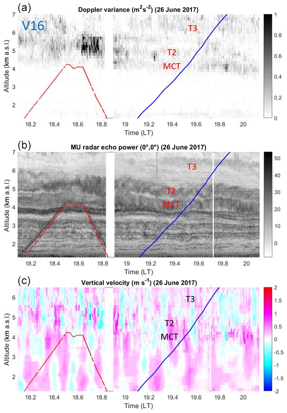
1992 H. Luce and H. Hashiguchi: On the estimation of vertical air velocity
tween W and the vertical air velocities deduced from VB (see
Sect. 3).
3 Case studies
Three balloon flights (hereafter called V6, V14 and V16,
which correspond to UAV flight numbers SH14, SH29 and
SH31, respectively) performed during ShUREX2017 on 18
and 26 June 2017 are analyzed in detail. Figure 1 shows the
horizontal trajectories of the balloons up to the altitude of
7.0 km a.s.l. The nearly circular patterns of the UAV trajecto-
ries are also shown. The MU radar is at the position (0, 0).
The balloons were intentionally underinflated with respect
to standard procedures in order to get a mean ascent rate of
∼ 2 m s−1 similar to the vertical ascent rate of the UAVs.
V6, V14 and V16 reached the altitude of 7.0 km a.s.l. within
about 33, 52 and 53 min, respectively, and their mean verti-
cal ascent rates were about 3.3, 2.1 and 2.1 m s−1 . V6 each
drifted by less than 15 km southwestward when reaching the
altitude of 7.0 km. V14 and V16 drifted by about 30 km
mainly eastward due to the influence of the subtropical jet
stream.
3.1 Analysis of the radar data
Time–height cross sections of MU radar Doppler variance
σ 2 (m2 s−2 ), echo power (dB) and vertical velocity (m s−1 )
around the times of the UAV and balloon flights in the height
range 1.27–7.0 km are shown in Figs. 2, 3 and 4 for V14,
V16 and V6, respectively (they are not shown in time or-
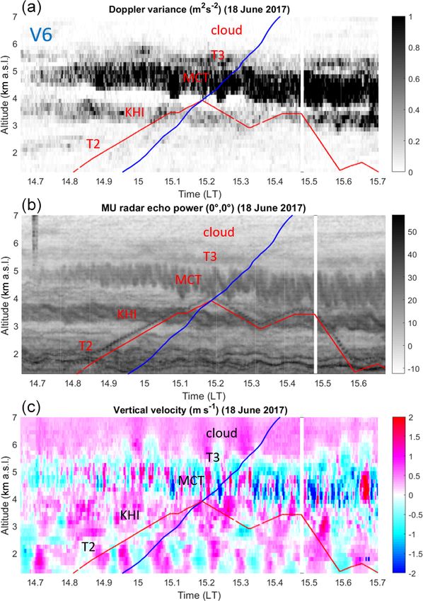
Figure 2. (a) Time–height cross section of variance of the Doppler
der for ease of the description made below). The red and spectrum peaks corrected from the beam-broadening effects ob-
blue lines indicate the altitude of the UAVs and balloons tained from MU radar measurements during balloon flight V14 and
vs. time, respectively. For easy reference, the most promi- UAV flight SH29. The altitudes of V14 and SH29 vs. time are given
nent and persisting turbulent layers identified from enhanced by blue and red lines, respectively. (b) Same as top for radar echo
Doppler variance (or ε (MU)) and UAV-derived ε are labeled. power (dB) in range imaging mode. (c) Same as top for vertical ve-
The source of these layers is sometimes recognizable from locity (m s−1 ). The white vertical lines are due to radar stops. See,
the morphology of the corresponding radar echoes in the e.g., Luce et al. (2018) for more details about these figures. Labels
high-resolution power images. When this is the case, the la- refer to the location of turbulent layers.
bels indicate the nature of the instabilities that gave rise to
turbulence; otherwise the labels are “T1”, “T2”, etc. “KHI”,
“MCT” and “CBL” refer to sheared-flow Kelvin–Helmholtz (Fig. 2). The atmosphere was weakly turbulent between the
instability (e.g., Fukao et al., 2011), mid-level cloud-base tur- CBL and MCT, but two events (T1 and T2) persisted around
bulence (e.g., Kudo et al., 2015) and convective boundary 2.3 km and between 4.0 and 4.5 km. The V16 case was also
layer, respectively. The presence of saturated air is also indi- characterized by weak turbulence below 3.5–4.0 km and at
cated by the label “cloud”. Note that enhanced σ 2 does not least three well-defined layers associated with MCT and two
necessarily imply enhanced echoes (e.g., T1 in Fig. 2 and T2 instabilities within clouds (T2 and T3 in Fig. 3). The V6 case
in Fig. 4) because turbulence can sometimes produce faint showed enhanced turbulence at almost all altitudes (Fig. 4),
echoes surrounded by enhanced echoes at their edges (e.g., but distinct layers can be clearly noted: MCT around 5.0 km,
McKelley et al., 2005). The CBL in Fig. 2 is only guessed KHI around 3.5 km (braided structures are clearly visible
because the CBL top only slightly exceeded the altitude of around 15:00 LT), and less intense events around 2.5 km (T2)
the first radar gate, but it was confirmed by the UAV obser- and just above the cloud base (T3). Turbulent layers (T1) de-
vations. tected from UAV data below 1.27 km are not indicated on the
The V14 case was characterized by weak turbulence ex- figures.
cept below ∼ 1.3 km (CBL) and above ∼ 5.0 km (MCT)
Atmos. Meas. Tech., 13, 1989–1999, 2020 www.atmos-meas-tech.net/13/1989/2020/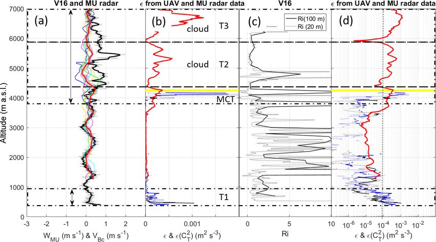
H. Luce and H. Hashiguchi: On the estimation of vertical air velocity                                                      1993

Figure 3. Same as Fig. 2 for SH31 and V16.                        Figure 4. Same as Fig. 2 for SH14 and V6.

   Rapid W fluctuations (of a period of ∼ 1 min) are gener-          The balloon ascent rate in still air Vz was estimated from
ally associated with MCT events. Nearly monochromatic os-         the difference between W and VB when turbulence was weak
cillations of W likely due to ducted gravity waves can also be    and the Richardson number was high. Vz was found to be
noted below 2.5–3.0 km during V16 and V6 (Figs. 3 and 4).         1.8, 1.8 and 2.3 m s−1 for V14, V16 and V6, respectively,
Their periods are about 9 and 6 min, respectively. The am-        and VBc = VB − Vz is shown in the figures. Indeed, the verti-
plitude of W did not exceed ∼ 0.5 m s−1 except in the MCT         cal fluctuations of VBc coincide well with those of W outside
layer during V6 where W fluctuated between ±2.0 m s−1 .           the labeled turbulent layers, indicating that the variations in
                                                                  balloon ascent rate are dominated by the vertical air motions
3.2   Profile comparisons                                         when turbulence is “sufficiently weak”. This is particularly
                                                                  evident in Fig. 6 in the height range 1.3–3.8 km where the
The results of comparisons between VB and atmospheric pa-         wavy fluctuations in W (of ∼ 0.5 m s−1 in amplitude) coin-
rameter profiles are shown for V14, V16 and V6 in Figs. 5, 6      cide very well with those of VBc . Several radar estimates of
and 7, respectively. Panels (a) show vertical velocity profiles   W are shown for different time lags. Each time lag is a mul-
from MU radar data and radiosondes. Panels (b) and (d) show       tiple of ∼ 9 min, which corresponds to the apparent period
UAV- and radar-derived ε profiles in linear and logarithmic       of the wave in the radar image (Fig. 3). The fluctuations of
scales, respectively. Both representations are shown for ease     W and VBc are in phase. The W profile suggests that the os-
of analysis. Panels (c) show Richardson number Ri profiles        cillations still occurred above 3.8 km in the MCT layer. The
defined as Ri = N 2 /S 2 , where N is the Brunt–Väisälä fre-      VBc profile indicates enhanced values of up to +1.8 m s−1 at
quency and S the vertical shear of horizontal wind, estimated     5.5 km that are clearly not related to vertical air motions.
from balloon data at 20 and 100 m resolution. Two vertical           In contrast, wherever UAV- and radar-derived ε estimates
resolutions are used because Ri is scale-dependent (Balsley       are enhanced in the labeled height ranges, VBc is also en-
et al., 2008).                                                    hanced and VBc and W strongly differ. Note that the UAV

www.atmos-meas-tech.net/13/1989/2020/                                               Atmos. Meas. Tech., 13, 1989–1999, 2020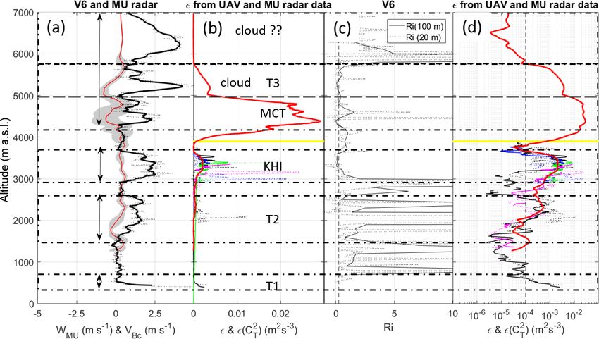
1994                                                       H. Luce and H. Hashiguchi: On the estimation of vertical air velocity

Figure 5. (a) Vertical profile of VBc (m s−1 ) (solid black: smoothed; dotted black: raw) for V14 and WMU (m s−1 ) (red). The gray area shows
the standard deviation of WMU over the averaging time (2 min). The vertical arrows indicate the altitude ranges affected by turbulence.
(b) Vertical profiles of TKE dissipation rates ε obtained from MU radar measurements (red) and UAV measurements during ascent and
descent (black and blue) and using the direct and indirect methods (solid and dashed lines). The maximum altitude reached by the UAV is
shown by the horizontal gray line. (c) Vertical profiles of Richardson numbers at a resolution of 20 m (dashed) and 100 m (solid). The vertical
dashed line indicates Ri = 0.25. (d) Same as (b) in log scale. The vertical dashed line indicates the value of ε = 10−4 m2 s−3 .

profiles of ε during ascents and descents are very similar and            are likely dominant. On some occasions, an increase in VBc
there is a good agreement with the radar-derived profiles ob-             might be due solely to turbulence effects, as in T1 of V14
tained during the balloon flights. Therefore, we can reason-              (Fig. 5) since W does not show any particular variations in
ably assume that these profiles are representative of the tur-            the range of T1.
bulence conditions met by the balloons. In general, the height               In the present cases, ε ∼ 10−4 m2 s−3 seems to be a thresh-
ranges of enhanced ε coincide with minima of Ri, close to                 old below which turbulence does not seem to affect the bal-
the critical value of 0.25, as expected for shear-generated tur-          loon ascent rate significantly. However, this value is likely
bulence (e.g., KHI in Fig. 7), or even less than 0, expected for          specific to the present observations and may not be applica-
MCT. Ri is not necessarily small over the whole depth of the              ble to other conditions.
layers (e.g., around 6.0 km in Fig. 5) and is surprisingly high
for the whole depth of T2 in Fig. 7, but the overall results
remain consistent. A puzzling result can be noted above the               4   Statistics
cloud base (6.0 km) during V6 (Fig. 7, as indicated by “??”)
                                                                          The case studies strongly suggest that increased balloon as-
where a strong increase in VBc (∼ 4 m s−1 ) was neither as-
                                                                          cent rates are generally related to minimum values of the
sociated with an increase in W nor an increase in turbulence
                                                                          Richardson number (negative or smaller than ∼ 0.25 consis-
according to MU radar observations. A slowdown of the bal-
                                                                          tent with convective overturning or shear-generated instabil-
loon due to precipitation loading would rather be expected.
                                                                          ities in stratified conditions, respectively). This observation
This thus remains unexplained and, by default, we must in-
                                                                          can be confirmed by analyzing the relationship between VBc
voke horizontal inhomogeneity of W and/or turbulence in-
                                                                          and Ri from a large amount of data. For this purpose, we used
tensity over the horizontal distance between the radar and
                                                                          data from 376 radiosondes launched every 3 h in Indone-
the balloon (∼ 10 km). Similar features were not observed in
                                                                          sia (Bengkulu, November–December 2015) during a prelimi-
clouds during V14 and V16.
                                                                          nary Years of the Maritime Continent (YMC) campaign (e.g.,
   These case studies provide experimental evidence that tur-
                                                                          Kinoshita et al., 2019). The choice of this dataset is arbitrary,
bulence can strongly increase the balloon ascent rate, very
                                                                          but it ensures that the same type of balloons (TOTEX-TA
likely through the decrease in the drag coefficient. The ob-
                                                                          200) and radiosondes (RS92SGPD) were used with similar
served VBc is thus the combination of turbulence effects and
                                                                          procedures of balloon inflation for all the datasets. Figure 8
vertical air velocities. Because W fluctuations appear sig-
                                                                          shows all the VB profiles with a slight offset for legibility.
nificantly weaker than VBc fluctuations, turbulence effects
                                                                          The balloons were inflated in order to get a mean ascent rate

Atmos. Meas. Tech., 13, 1989–1999, 2020                                                       www.atmos-meas-tech.net/13/1989/2020/
H. Luce and H. Hashiguchi: On the estimation of vertical air velocity 1995 Figure 6. Same as Fig. 5 for V16. Figure 7. Same as Fig. 5 for V6. of 5 m s−1 (free lift). During the period of observations, the weak variations or nearly monochromatic fluctuations un- tropical tropopause layer (TTL) was often characterized by a doubtedly due to internal gravity waves (Tsuda et al., 1994). strong temperature inversion just above the cold point tem- Therefore, we suggest that the variations in VB with height perature (CPT) around the altitude of 16–17 km (blue dots are primarily due to vertical air motions in the stratosphere in Fig. 8) and a secondary temperature inversion of similar and mainly due to turbulence effects in the troposphere. To intensity at slightly lower altitude (red dots). For ease of sta- assess this hypothesis, we analyzed the relationship between tistical analysis, we refer to altitude ranges 0–16.3 km as tro- Ri and VBc (VB corrected from the free lift). We calculated posphere and altitude ranges above 17.2 km (up to the top of (moist) Ri = Nm2 /S 2 , where Nm2 is the squared moist Brunt– the radiosoundings) as stratosphere. Väisälä frequency using expression (5) of Kirshbaum and The profiles of VB often display multiple peaks of variable Durran (2004) at a vertical resolution of 50 m, a reasonable widths in the troposphere especially in its upper part. In the trade-off between 20 and 100 m used for the case studies. stratosphere, the profiles are much smoother and show either Because VB seems to be weakly affected by turbulence in the www.atmos-meas-tech.net/13/1989/2020/ Atmos. Meas. Tech., 13, 1989–1999, 2020
1996                                                      H. Luce and H. Hashiguchi: On the estimation of vertical air velocity

Figure 8. Vertical profiles of VB from 376 consecutive balloons launched about every 3 h from 8 November to 27 December 2015 during the
pre-YMC campaign at Bengkulu (102.26◦ E, 3.79◦ S; Indonesia); 0.5 d corresponds to 5 m s−1 , and each profile was shifted by about 0.125 d
(1.25 m s−1 ). The cold point temperature tropopause and a secondary temperature inversion of similar intensity at lower altitude are shown
as blue and red dots, respectively.

stratosphere, the mean value of VB for stratospheric heights,
hVB iST , is expected to be a fair estimate of the ascent rate in
still air (Vz ), assuming that wave contribution is indeed re-
moved after averaging and that other contributions are negli-
gible. Thus, we have VBc = VB −hVB iST . The value of hVB iST
was calculated for each flight and removed from each profile
of VB in order to reduce the effects of variable mean ascent
rates that may result from different balloon inflations. The
mean value of hVB iST over the 376 flights was found to be
precisely equal to the nominal value of 5 m s−1 .
   First, the scatterplot of VBc vs. Ri shows a very significant
maximum around and below the critical value of Ric ∼ 0.25
in the troposphere (Fig. 9a). This is an indirect confirma-
tion that VBc peaks are indeed due to turbulence (Fig. 9a),
considering that small Ri values are generally associated
with turbulence. Second, this increase is accompanied by a
larger scatter. There is no similar tendency in the stratosphere
(Fig. 9b) because Ri rarely dropped below Ric , in accor-
dance with the absence of significant turbulence ascertained
from the profiles of VB . The increased variability of VBc with
                                                                        Figure 9. (a) Scatterplot of VBc = VB − hVB iST versus moist Ri
decreasing Ri in Fig. 9b should mainly be due to waves.
                                                                        for the troposphere. (b) Same as (a) for the stratosphere. (c) Mean
   In order to emphasize the tendency shown by Fig. 9a and b,           values of VBc in Ri bands of 0.25 in width for the troposphere.
averaged values of VBc in Ri value bands of 0.25 in width,              (d) Same as (c) for the stratosphere. The vertical red lines show
hVBc i, are shown in Fig. 9c and d, respectively. For Ri&1,             Ric = 0.25.
hVBc i is roughly constant but slightly negative: ∼ −0.2 m s−1
(Fig. 9c) because hVB iST is likely not exactly the ascent rate
in still air in the troposphere. This is not an important issue         stratosphere (Fig. 9d) due to the lack of data. The results
for the present purpose. When Ri drops below Ric , hVBc i               shown in Fig. 9c constitute a statistical confirmation of the
increases by ∼ +0.9 m s−1 and remains high when Ri < 0                  observations reported in Sect. 3.
(Fig. 9a). The values for Ri < Ric are not reliable in the

Atmos. Meas. Tech., 13, 1989–1999, 2020                                                    www.atmos-meas-tech.net/13/1989/2020/
H. Luce and H. Hashiguchi: On the estimation of vertical air velocity 1997
not be measured because VB is very likely affected by the de-
crease in the drag coefficient cD of the balloon. In contrast, in
the calm regions of the atmosphere, the fluctuations of VB are
dominated by the fluctuations of W . These conditions were
probably met by, e.g., Corby (1957) and Reid (1972) and are
most likely met in the lower stratosphere (Shutts et al., 1988;
Reeder et al., 1999). This was also the case during the condi-
tions analyzed by Wang et al. (2009) above the CBL. How-
ever, in light of our observations, we speculate that Wang et
al. (2009) also detected turbulent layers: localized increases
in VB (up to ∼ 2 m s−1 ) observed in the height range 8–10 km
(their Fig. 1) may be attributed to turbulent layers. McHugh
et al. (2008) interpreted isolated peaks of VB of several me-
ters per second of amplitude near the tropopause and at the
jet-stream level in terms of W disturbances around critical
levels associated with mountain waves. The absence of cor-
Figure 10. Same as Fig. 9a after removing the mean tendency responding negative disturbances was explained by the three-
shown by Fig. 9c for the troposphere. The vertical dashed line shows
dimensional nature of the flow. Even though our hypothesis
Ric = 0.25.
remains speculative in the absence of additional and indepen-
dent measurements of vertical air velocity, we suggest that
Figure 10 show VBc − hVBc i vs. Ri for the troposphere. turbulence effects may have also contributed to the observed
A larger scatter is observed between Ri = 0 and Ric = 0.25. increase in ascent rates since critical levels are generally as-
The broadening of the scatter was attributed to turbulence by sociated with turbulence. A careful scrutiny of their Figs. 3–7
Houchi et al. (2015). However, the broadening cannot be ex- indicates that VB increased at altitudes where the horizontal
plained by a decrease in the drag coefficient because it is nec- wind shear was enhanced and temperature gradient was close
essarily due to both positive and negative vertical velocities. to adiabatic (so that Ri was likely small). Houchi et al. (2015)
The broadening is thus more likely due to turbulent billows of attributed the spread of the height increment “dz” probabil-
scales much larger than the balloon size. In addition, Kelvin– ity density function to “turbulence”. The authors likely im-
Helmholtz (KH) waves can also produce updrafts and down- plicitly referred to advection by large-scale billows. The de-
drafts of up to a few meters per second when Ri reaches Ric crease in the drag coefficient due to turbulence can explain
(see, e.g., Fukao et al., 2011). Therefore, the enhanced vari- the upward-only motion anomaly noticed by the authors.
ability of VBc when Ri is small (Fig. 9a) is presumably the It turns out that VB can also potentially be used for the de-
combination of turbulence effects and vertical air motion dis- tection of turbulence in the free atmosphere if the increase
turbances produced by large-scale billows and KH waves. in VB can be separated from the contribution of W . Turbu-
Finally, it can be noted that the scatterplot of VBc − hVBc i lence is frequent in the free atmosphere but also very variable
(Fig. 10) is not symmetrical about 0 for Ri > 1 (for which with height and generally distributed in layers, especially in
turbulence is expected to be suppressed) and suggests peaks stratified conditions. This feature was likely not well appreci-
of VB (without corresponding negative disturbances) even in ated by Gallice et al. (2011). The authors themselves recog-
the absence of turbulence. However, this result must be tem- nized that their model cannot work if localized turbulence –
pered by the fact that turbulence can be observed even if the they proposed the example of turbulence generated by grav-
estimation of Ri at a given resolution is not small (see, e.g., ity wave breaking – occurs.
Fig. 7, T2). Measurement and estimation errors of tempera- The amplitude of the VB disturbances should depend on
ture, humidity and winds cannot be discarded on some occa- the variation in cD with the Reynolds number, the intensity
sions and Nm2 may not be the appropriate parameter for all of turbulence and on the scales of turbulence with respect to
conditions. For all these reasons, this observation may not be the balloon size so that it might be difficult or even impos-
indicative of more complex interactions between the balloon sible to retrieve turbulence parameters solely from VB mea-
and the surrounding atmosphere. surements. However, further comparisons such as shown in
Sect. 3 might be useful for establishing empirical rules on the
turbulence detection threshold.
5 Discussion and conclusions
We have found that the possibility of retrieving the vertical Data availability. The balloon data are archived at the YMC Data
air velocity W from radiosonde ascent rate VB highly de- Archive Center maintained by JAMSTEC (http://www.jamstec.go.
pends on the turbulent state of the atmosphere. In turbulent jp/ymc/ymc_data.html, JAMSTEC, 2020). The radar and UAV data
layers generated by shear or convective instabilities, W can- are still under processing for other purposes.
www.atmos-meas-tech.net/13/1989/2020/ Atmos. Meas. Tech., 13, 1989–1999, 20201998 H. Luce and H. Hashiguchi: On the estimation of vertical air velocity
Author contributions. HL, with the help of HH, conceived of the with some preliminary results, Prog. Earth Planet. Sci., 4, 19,
study, carried out the analysis and retrievals, and wrote the paper. doi10.1186/s40645-017-0133-x, 2017.
Kinoshita, T., Shirooka, R., Suzuki, J., Ogino, S.-Y., Iwasaki,
S., Yoneyama, K., Haryoko, U., Ardiansyah, D., and Alyudin,
Competing interests. The authors declare that they have no conflict D.: A study of gravity wave activities based on intensive
of interest. radiosonde observations at Bengkulu during YMC-Sumatra
2017, IOP Conf. Series: Earth and Environmental Science,
10–14 December 2018, Washington, D.-C., 303, 012011,
Acknowledgements. The radiosonde data were collected as part of https://doi.org/10.1088/1755-1315/303/1/012011, 2019.
YMC by JAMSTEC, BMKG and BPPT. These data are archived Kirshbaum, D. J. and Durran, D. R.: Factors governing cellular con-
at the YMC Data Archive Center in JAMSTEC. UAV data were vection in orographic precipitation, J. Atmos. Sci., 61, 682–698,
provided by Dale Lawrence, Abhiram Doddi and Lakshmi Kantha 2004.
from the University of Colorado. Kudo, A., Luce, H., Hashiguchi, H., and Wilson, R.: Convective in-
stability underneath midlevel clouds: Comparisons between nu-
merical simulations and VHF radar observations, J. Appl. Mete-
orol. Clim., 54, 2217–2227, 2015.
Financial support. This research has been supported by the JSPS
Lalas, D. P. and Einaudi, F.: Tropospheric gravity waves: Their de-
KAKENHI (grant no. JP15K13568) and the research grant for Mis-
tection by and influence on Rawinsonde balloon data, Q. J. Roy.
sion Research on Sustainable Humanosphere from the Research In-
Meteor. Soc., 109, 855–864, 1980.
stitute for Sustainable Humanosphere (RISH), Kyoto University.
Luce, H., Kantha, L., Hashiguchi, H., and Lawrence, D.: Turbu-
lence kinetic energy dissipation rates estimated from concurrent
UAV and MU radar measurements, Earth Planets Space, 70, 207,
Review statement. This paper was edited by Ad Stoffelen and re- https://doi.org/10.1186/s40623-018-0979-1, 2018.
viewed by Ad Stoffelen. Luce, H., Kantha, L., Hashiguchi, H., and Lawrence, D.: Esti-
mation of Turbulence Parameters in the Lower Troposphere
from ShUREX (2016–2017) UAV Data, Atmosphere, 10, 384,
https://doi.org/10.3390/atmos10070384, 2019.
McHugh, J. P., Dors, I., Jumper, G. Y., Roadcap, J. R., Mur-
References phy, E. A., and Hahn, D. C.: Large variations in balloon
ascent rate over Hawaii, J. Geophys. Res., 113, D15123,
Balsley, B. B., Svensson, G., and Tjernström, M.: On the scale https://doi.org/10.1029/2007JD009458, 2008.
dependence of the gradient Richardson number in the residual McKelley, C., Chen, Y., Beland, R. R., Woodman, R., Chau, J.
layer, Bound.-Lay. Meteorol., 127, 57–72, 2008. L., and Werne, J.: Persistence of a Kelvin-Helmholtz instabil-
Corby, G. A.: A preliminary study of atmospheric waves using ra- ity complex in the upper troposphere, J. Geophys. Res., 110,
diosonde data, Q. J. Roy. Meteor. Soc., 83, 49–60, 1957. D14106, https://doi.org/10.1029/2004JD005345, 2005.
Fritts, D. C., Bizon, C., Werne, J. A., and Meyer, C. K.: Lay- Muschinski, A.: Possible effect of Kelvin-Helmholtz instability on
ering accompanying turbulence generation due to shear insta- VHF radar observations of the mean vertical wind, J. Appl. Me-
bility and gravity-wave breaking, J. Geophys. Res., 108, 8452, teorol.,35, 2210–2217, 1996.
https://doi.org/10.1029/2002JD002406, 2003. Röttger, J. and Larsen, M. F.: UHF/VHF radar techniques for at-
Fukao, S., Luce, H., Mega, T., and Yamamoto, M. K.: Exten- mospheric research and wind profiler applications, in: Radar in
sive studies of large-amplitude Kelvin–Helmholtz billows in the Meteorology, edited by: Atlas, D., American Meteorological So-
lower atmosphere with VHF middle and upper atmosphere radar, ciety, Boston, MA, USA, Chapter 21a, 1990.
Q. J. Roy. Meteor. Soc., 137, 1019–1041, 2011. Reid, S. J.: An observational study of lee waves using radiosonde
Gallice, A., Wienhold, F. G., Hoyle, C. R., Immler, F., and Pe- data, Tellus, 24, 593–596, 1972.
ter, T.: Modeling the ascent of sounding balloons: derivation Reeder, M. J., Adams, N., and Lane, T. P.: Radiosonde observations
of the vertical air motion, Atmos. Meas. Tech., 4, 2235–2253, of partially trapped lee waves over Tasmania, Australia, J. Geo-
https://doi.org/10.5194/amt-4-2235-2011, 2011. phys. Res., 104, 16719–16727, 1999.
Houchi, K., Stoffelen, A., Marseille, G.-J., and De Kloe, J.: Sta- Shutts, G. J., Kitchen, M., and Hoare, P. H.: A large amplitude grav-
tistical quality control of high-resolution winds of different ra- ity wave in the lower stratosphere detected by radiosonde, Q. J.
diosonde types for climatology analysis, J. Atmos. Ocean. Tech., Roy. Meteor. Soc., 114, 579–594, 1988.
32, 1796–1812, 2015. Söder, J., Gerding, M., Schneider, A., Dörnbrack, A., Wilms,
JAMSTEC: YMC radiosonde data (site name), available at: H., Wagner, J., and Lübken, F.-J.: Evaluation of wake influ-
http://www.jamstec.go.jp/ymc/ymc_data.html, last access: ence on high-resolution balloon-sonde measurements, Atmos.
16 April 2020. Meas. Tech., 12, 4191–4210, https://doi.org/10.5194/amt-12-
Johansson, C. and Bergström, H.: An auxiliary tool to determine 4191-2019, 2019.
the height of the boundary layer, Bound.-Layer Meteorol., 115, Son, K., Choi, J., Jeon, W., and Choi, H.: Effect of free-stream
423–432, 2005. turbulence on the flow over a sphere, Phys. Fluids, 22, 045101,
Kantha, L., Lawrence, D., Luce, H., Hashiguchi, H., Tsuda, T., https://doi.org/10.1063/1.3371804, 2010.
Wilson, R., Mixa, T., and Yabuki, M.: Shigaraki UAV-Radar
Experiment (ShUREX 2015): An overview of the campaign
Atmos. Meas. Tech., 13, 1989–1999, 2020 www.atmos-meas-tech.net/13/1989/2020/H. Luce and H. Hashiguchi: On the estimation of vertical air velocity 1999
Tsuda, T., Murayama, Y., Wiryosumarto, H., Harijono, S. W. B., Worthington, R. M., Muschinski, A., and Balsley, B. B.: Bias in
and Kato, S.: Radiosonde observations of equatorial atmosphere mean vertical wind measured by VHF radars: significance of
dynamics over Indonesia: 2. Characteristics of gravity waves, J. radar location relative to mountains, J. Atmos. Sci., 58, 707–723,
Geophys. Res., 99, 10507–10516, 1994. 2001.
Wang, J., Bian, J., Brown, W. O., Cole, H., Grubisic, V., and Young, Yamamoto, M. K., Fujiwara, M., Horinouchi, T., Hashiguchi,
K.: Vertical air motion from T-REX radiosonde and dropsonde H., and Fukao, S.: Kelvin-Helmholtz instability around
data, J. Atmos. Ocean. Tech., 26, 928–942, 2009. the tropical tropopause observed with the Equato-
rial Atmosphere Radar, Geophys. Res. Lett., 30, 1476,
https://doi.org/10.1029/2002GL016685, 2003.
www.atmos-meas-tech.net/13/1989/2020/ Atmos. Meas. Tech., 13, 1989–1999, 2020You can also read