Computing the Death Rate of COVID-19
←
→
Page content transcription
If your browser does not render page correctly, please read the page content below
Computing the Death Rate of COVID-19

                                            Naveen Pai[0000−0002−5980−560X] , Sean Zhang[0000−0003−1699−1809] , and Mor
                                                               Harchol-Balter[0000−0003−1721−6759] ?

                                                           {nvpai, xiaoronz, harchol}@andrew.cmu.edu
                                                                    Carnegie Mellon University
arXiv:2109.13733v1 [cs.CY] 9 Sep 2021

                                        Abstract

                                        The Infection Fatality Rate (IFR) of COVID-19 is difficult to estimate because
                                        the number of infections is unknown and there is a lag between each infection and
                                        the potentially subsequent death. We introduce a new approach for estimating
                                        the IFR by first estimating the entire sequence of daily infections. Unlike prior
                                        approaches, we incorporate existing data on the number of daily COVID-19 tests
                                        into our estimation; knowing the test rates helps us estimate the ratio between
                                        the number of cases and the number of infections. Also unlike prior approaches,
                                        rather than determining a constant lag from studying a group of patients, we
                                        treat the lag as a random variable, whose parameters we determine empirically
                                        by fitting our infections sequence to the sequence of deaths. Our approach allows
                                        us to narrow our estimation to smaller time intervals in order to observe how
                                        the IFR changes over time. We analyze a 250 day period starting on March
                                        1, 2020. We estimate that the IFR in the U.S. decreases from a high of 0.68%
                                        down to 0.24% over the course of this time period. We also provide IFR and
                                        lag estimates for Italy, Denmark, and the Netherlands, all of which also exhibit
                                        decreasing IFRs but to different degrees.

                                        1     Introduction

                                        The COVID-19 pandemic has raged for over a year now, greatly disrupting the
                                        lives of people all over the world. While much research has been done on modeling
                                        the spread of the disease, one particular question that remains unresolved is:
                                        What is the death rate of COVID-19?
                                            A good estimate for the death rate could better inform government policies,
                                        but it has been surprisingly difficult to estimate the death rate [5]. When we talk
                                        about the “death rate” we will be talking about the probability that an infected
                                        person ends up dying. This is formally called the Infection Fatality Rate (IFR)
                                        and will be defined in Section 3.
                                        ?
                                            This research was supported by NSF-CMMI-1938909, NSF-CSR-1763701, and a
                                            Google 2020 Faculty Research Award.
2         Naveen Pai, Sean Zhang, and Mor Harchol-Balter

1.1     Challenges in estimating the death rate

Several challenges arise in estimating the death rate. These include:
    Cases are recorded, not infections: Estimating the death rate requires
knowing the number of deaths relative to the number of infections. Unfortu-
nately, what is reported is the number of daily cases, not the number of daily
infections. Note that a case is a test that results in a positive, however not all
infected people are necessarily tested. Thus, determining the death rate firstly
involves creating some estimate of the number of infections. One might think
that testing can provide such an estimate, but testing is not randomized [19], so
the proportion of test-takers who are infected is not indicative of the infection
rate in the overall population.
    Lag between cases and deaths: In this paper we refer to the time between
when a person tests positive (a case) and the potentially subsequent death as
the lag time1 . Unfortunately, this lag time varies for each individual. To make
matters worse, lag time is also affected by larger trends, such as the age group
that is most commonly infected and the treatments that are available [9]. Thus,
the mean lag time may change as the pandemic progresses.
    The testing rate is not constant: The number of daily cases can provide
insight into the number of infections. However, the number of cases also depends
on the rate at which people get tested for COVID. Higher testing rates lead to
more cases being observed. The fact that the testing rate has varied greatly over
time [14] makes it difficult to interpret the number of cases.
    The death rate varies over time: The death rate is itself not constant
over time. The death rate goes down when hospitals find new treatments, but
then it shoots back up when hospitals get overloaded and run out of workers,
oxygen, or ventilators [4]. The death rate grows when older people in nursing
homes are being most commonly infected, but shrinks when younger people are
most commonly infected [4]. Because the death rate varies, simply trying to fit
one number to all the data is not necessarily the best approach.
    Reported numbers are not always accurate: Finally, we are always
dealing with reported numbers, not true numbers. It is well known that in many
states there is a delay in recording deaths and reporting them [10]. Some COVID
cases never get reported at all. For example, a person may die from COVID
without ever being tested [20]. Finally, there are both false positives and false
negatives in the reported cases [8].
    Antibodies can wear off: People who were infected and recovered may lose
their antibodies after a few months [1]. This makes it difficult to use antibody
studies to estimate how many people have been infected by COVID.

1
    In some literature, lag is described as the time from initial infection to death, but
    such studies involve only a small group of patients, for whom the initial infection
    time is approximately known. In general it is impossible to ascertain the time of the
    initial infection from large-scale reports.
Computing the Death Rate of COVID-19           3

1.2   Prior approaches to estimating the death rate

There has been some prior work on determining the death rate, either within
the U.S., or in other countries (see Section 2 for details). Much of the prior work
is not actually looking at the Infection Fatality Rate (IFR), but rather at the
Case Fatality Rate (CFR), which is the fraction of positive cases that result in
deaths. Our goal in this paper is to determine the IFR.
    For those works that do directly try to measure the IFR, most follow this
simplistic 2-step approach which is not time-dependent:

 1. Estimate the total number of infections by time t by looking at the results
    of antibody tests at time t.
 2. Divide the total number of deaths by time t (this is easily found in reports)
    by the total number of infections by time t from the previous step. This
    yields the estimated death rate during the period [0, t].

Sometimes the authors go a step further, by incorporating a lag between the
case and death (or the infection and death). But this lag is often assumed to be
a fixed constant value, estimated via small in-person studies.

1.3   Drawbacks of the prior approaches

There are several drawbacks to prior approaches. Firstly, the prior approaches
are people-intensive, which is costly. Secondly, the prior approaches are limited
in what they can produce. The IFR can only be estimated on days when an
antibody study was conducted. To make matters worse, antibody studies become
less accurate over time, since people lose antibodies, causing an underestimate of
past infections [1]. But the biggest drawback of the prior work is that it doesn’t
take into account the changes in the pandemic. As we’ve explained, the lag time
changes over time. The IFR itself changes over time. Prior approaches are not
well-suited to take these temporal changes into account.

1.4   A new data-driven approach to estimating the death rate

In this paper we present a data-driven approach. Unlike prior approaches, our
method does not rely on having a set of patients whom we can track and study.
Instead, our approach is solely based on studying readily available numbers on
Our World in Data [7] along with a single antibody study that can be con-
ducted at an arbitrary time. By relying on a single antibody study, we can
ignore later antibody studies which underestimate infections due to antibodies
fading. Secondly, our approach easily admits temporal changes; in particular, we
incorporate changes in the lag distribution, changes in the testing rate, and a
time-varying IFR. The data that we use includes the sequence of daily deaths,
daily cases, and daily tests, over a period of 250 days beginning with March 1,
2020, as well as antibody results that were available two or three months after
March 1, 2020.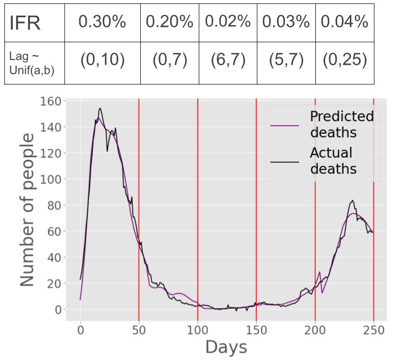
4       Naveen Pai, Sean Zhang, and Mor Harchol-Balter

    Our first key idea is that we need to estimate the entire sequence of daily
infections. The sequence itself is needed because it allows us to see how the IFR
changes over time and to study the temporal changes in the lag time distribution.
    Our second key idea is that the sequence of daily infections can be approx-
imated using a function of both the daily cases and tests. This function is in-
creasing with respect to the number of cases but decreasing with respect to the
number of tests. It furthermore assumes that a person who is infected is more
likely to get tested than a person who is not infected. Section 4 explains the
intuition behind our function. We find that the appropriate parameters of the
function can be determined empirically via antibody results.
    Once we have our estimated infection sequence, our next key idea is that
we should determine the lag time and the IFR concurrently, not individually.
Every possible choice of lag time can be viewed as a time shift of the infection
sequence, while every possible choice of the IFR can be viewed as a vertical
scaling of the infection sequence. Together, every choice of lag time and IFR
results in a particular “candidate” death sequence. To find the “best” choice of
lag time and IFR, we simply pick the parameters which result in a candidate
death sequence which best fits the given death sequence in our data. We actually
take this idea a step further and allow the lag time to follow a distribution whose
parameters are incorporated in the above optimization process.
    Our final idea is that this entire optimization process is best done by seg-
menting time into intervals (we use intervals of 50 days), because we find that the
IFR and the lag time change over time. We repeat the above approach over sev-
eral different countries, starting with the U.S. and moving on to Italy, Denmark,
and the Netherlands. There is no reason why our approach can’t be applied to
other countries as well, provided that the data is available.

1.5   Synopsis of our Findings

Figure 1 illustrates a synopsis of our findings for the United States. In Figure
1(a), we see the sequence of daily cases (in blue), and above it we see our es-
timated daily infection sequence (in purple). Importantly, our estimated daily
infection sequence is not a mere vertical scaling. The reason why is that in de-
riving our infection sequence we incorporate the time-varying testing rate, not
shown here (see Section 7).
     In Figure 1(b), we illustrate our best “candidate” death sequence (which we
derive from our estimated infection sequence as described in Section 4), and
we compare it with the true death sequence. These two sequences are a good
fit, indicating that our estimated IFR and lag are accurate. We annotate the
top of Figure 1(b) with our estimated IFR and the lag distribution in days
for each 50-day interval. We find that the IFR decreases over time, eventually
changing from 0.68% to 0.24%. We find that the lag is well fit by a Uniform(a, b)
distribution, with a mean lag of about 8 days throughout the pandemic. Section
7 contains more details and also repeats this process for Italy, Denmark, and the
Netherlands.
Computing the Death Rate of COVID-19 5
(a) Cases (blue) and Esti- (b) Predicted Deaths (purple) and Ac-
mated infections (purple) tual Deaths (black)
Fig. 1. From cases to estimated infections to predicted IFR and lag in the U.S.
1.6 Road map for the rest of the paper
Section 2 discusses the prior work in more detail. In Section 3 we provide def-
initions and notation. Section 4 describes how we estimate a sequence of daily
infections based on reported sequences for daily cases, tests, and deaths. In Sec-
tion 5 we present our algorithm for calculating the IFR and lag time, and in
Section 6 we refine our algorithm to look at smaller time intervals. In Section
7, we apply our approach to various countries. We conclude in Section 8 and
discuss opportunities for future work.
2 Prior work and how we differ
Most prior work estimates CFR, the case fatality rate, rather than IFR,
which is the focus of this paper. Several studies estimate the CFR while adjusting
for lag between cases and deaths. Newall et al. [18] estimates the lag-adjusted
CFR using a lognormal distribution for the lag with mean 14.5 days, which was
estimated using the onset to death time of 34 patients, based on the case data
from the Diamond Princess cruise ship. Using a very similar approach, Russell
et al. [21] estimates the lag-adjusted CFR in South Korea. They used the first
66 deaths reported in South Korea to fit a lognormal distribution for the lag,
which is then used to compute the adjusted CFR.
By contrast our approach does not need the data of individual patients: we
estimate the lag distribution using the sequence of cases and deaths only, which
allows us to make use of a larger amount of data from different regions. We find
that assuming lag to be uniformly distributed yields a slightly better fit in our
model than assuming a lognormal distribution.
Prior work on estimating IFR: Regarding IFR, various studies attempt
to estimate this value using the data from antibody studies, in which a group6 Naveen Pai, Sean Zhang, and Mor Harchol-Balter
of patients is tested for antibodies in an attempt to estimate the fraction of
the total population that has been infected. The IFR is then estimated as the
ratio between the fraction of the population that died and the fraction that was
infected.
However, unlike our work, these studies do not incorporate knowledge of the
time-varying testing rate. By not taking into account the testing rate, they end
up with very different results than ours. Meyerowitz-Katz et al. [17] gives a
comprehensive review of such studies which estimate the IFR. In particular, one
study by Villa et al. [22] estimates an IFR of 1.1% for Italy up to the end of
March 2020. By contrast, our estimated IFR for Italy is 2.2% around March
2020.
Several studies, e.g., Levin et al. [15] and Marra and Quartin [16], take lag
into account in determining the IFR, but they assume a fixed lag. By contrast,
our work assumes a lag distribution with parameters that can vary by region and
by time. Our more flexible approach accounts for differences in the spread and
reporting of the disease.
3 Definitions and Notation
Throughout this document, the terms death rate and infection fatality rate (IFR)
are synonymous and are defined as follows: Consider a period of time t ∈ [a, b],
where a and b denote particular days. We consider the infections that occur dur-
ing [a, b] and the subsequent deaths, possibly after day b, that are a consequence
of those infections. We define:
# of people infected during [a, b] who died
IFR[a, b] = .
# of infections during the interval [a, b]
In this document, we will make use of publicly-available data on the number
of daily cases and the number of daily deaths in a range of countries [12] (recall
that a case denotes a positive test result). We let ~c = (c1 , . . . , ck ) be the time
series of new cases per day for each of the first k days. For our data, day 1
corresponds to March 1, 2020, and day k = 250 corresponds to November 6,
2020. Similarly d~ = (d1 , . . . , dk ) denotes the number of new deaths per day from
COVID for each of the first k days. We will also utilize reports of the number
of daily tests [14], which we denote by ~t = (t1 , . . . , tk ). We use ~i = (i1 , . . . , ik ) to
denote our estimated number of new infections per day.
4 Estimating the infections sequence
In this section, we explain how we determine our estimated sequence of infections:
~i = (i1 , . . . , ik ). At a high level, we start with the reported number of cases
each day: ~c = (c1 , . . . , ck ). We then incorporate the number of tests each day,
~t = (t1 , . . . , tk ) and also the results of a one-time antibody test. These three
pieces of information give us everything we need.Computing the Death Rate of COVID-19 7
We will make one simplifying assumption that is needed only for analytical
convenience but does not affect the derivation of IFR. Our assumption is that
if a person is infected on day j, they either get tested on day j, or never get
tested at all. In reality, they might be tested any time after day j, but it will
be convenient for us to assume that the testing happens on day j. Note that
this assumption will mean that our infections sequence will be slightly shifted
forward in time from the true infections sequence. However this will not affect
our IFR because, in fitting the infections sequence to the deaths sequence, we
still have a “lag” variable that lets us account for an arbitrary time from case
to death.
With this simplifying assumption in mind, let us consider an arbitrary day j.
Now let’s assume we pick a random person on day j. Let Ij be the event that this
i
randomly chosen individual becomes infected on day j. So P {Ij } = Nj where
N is the population of the country in consideration. Now let Tj be the event
t
that this same randomly chosen individual is tested on day j. So P {Tj } = Nj .
Conditional probability tells us that
P {Ij } · P {Tj |Ij } = P {Tj ∩ Ij } .
Notice that Tj ∩ Ij is the event that the randomly chosen individual is both
infected and tested on day j – meaning that the individual becomes a “case” on
c
day j (we assume that the test is always accurate). So P {Tj ∩ Ij } = Nj . Putting
this all together, we get that
ij cj
· P {Tj |Ij } = . (1)
N N
c
Thus we can approximate ij = P{Tjj|Ij } if we know P {Tj |Ij }.
Now P {Tj |Ij } represents the fraction of people who are tested, given that
they were infected on day j. We will approximate P {Tj |Ij } as being a function
t
of P {Tj }, since P {Tj } = Nj is a known quantity which should be closely related
to P {Tj |Ij }. To understand the relationship between P {Tj |Ij } and P {Tj }, we
first note that infected individuals are more likely to get tested than randomly
chosen individuals, since infected individuals may be prompted to get tested by
symptoms or contact-tracing. So P {Tj |Ij } > P {Tj }. Now consider the ratio
between P {Tj |Ij } and P {Tj }. This ratio should be highest (
1) when P {Tj }
is low, because when testing is scarce only people with symptoms will be tested.
This ratio should be lowest (converging to 1) when P {Tj } gets high, because
at that point, everyone is being tested, regardless of whether they’re infected or
not.
Figure 2 illustrates a family of possible relationship between P {Tj |Ij } and
P {Tj } that satisfies all these intuitions:
P {Tj |Ij } = (P {Tj })1/m . (2)
We will assume this functional relationship holds for some parameter m, and
determine the appropriate m empirically. We tried many possible functions, and8 Naveen Pai, Sean Zhang, and Mor Harchol-Balter
Fig. 2. Red and pink solid curves show our assumed relationship between P {Tj |Ij }
and P {Tj }, from Equation 2, for a few values of m.
found that the family of curves in Equation 2 yielded the best fit in all of the
countries we tried. Thus, via Equation 1 and Equation 2, we conclude the fol-
lowing relationship between ij , cj , and tj :
cj
ij = 1/m . (3)
tj
N
We will now propose a method for empirically inferring the correct value of
m > 1. An antibody study tells us, for some day `, the number of people A who
were infected prior to day `. Our estimated infections sequence should agree with
this figure. Thus we can search for a value of m for which:
` `
X X cj
ij = 1/m ≈ A . (4)
tj
j=1 j=1
N
P` cj
Notice that j=1 tj 1/m is decreasing with respect to m. So, in practice, to
N
find the appropriate value of m, we can do a binary search for m, repeatedly
P` c
evaluating j=1 tj j1/m until Equation 4 is satisfied.
N
5 Inferring IFR and lag using the infections sequence and
deaths sequence
At this point, we know our estimated sequence of infections ~i = (i1 , . . . , ik ). In
this section, we describe our approach for estimating lag and IFR concurrently.
Our high-level approach is as follows: We assume that the lag time between
infections and deaths is a random variable L following a Uniform(a, b) distribu-
tion with unknown parameters, a and b, that we will determine.2 We start with
2
We also considered other distributions for lag, such as the LogNormal(µ, σ 2 ) and
Binomial(n, p), but the best results were achieved with the Uniform(a, b).Computing the Death Rate of COVID-19 9
the infections sequence ~i. Consider shifting ~i by a particular lag distribution, L,
and then vertically scaling the shifted sequence by a particular IFR3 . The shifted
and then scaled sequence is what we call a candidate death sequence. We want
to choose the candidate death sequence (with its corresponding IFR and L) that
best fits the actual death sequence, d~ = (d1 , . . . , dk ). We return the “best-fit” L
and IFR as our final estimate. Part of our process will involve iterating over all
possible values for (a, b), assuming some generous upper bound on the lag.
We now explain our approach in more detail. We first define a time shift,
SL (~i), algorithmically. For each infection in ~i, we will sample a new instance
` from L and shift the infection forward by ` days. This produces a sequence
SL (~i) = (I1 , I2 , I3 , . . . , Ik ) where each entry is a random variable denoting the
number of shifted infections that fall on that day.
Before we can compare the sequence of random variables, SL (~i), to the actual
death sequence d, ~ we need to turn SL (~i) into a deterministic sequence, S̄L (~i).
We define the unscaled candidate death sequence, S̄L (~i) as
S̄L (~i) ≡ (E [I1 ] , E [I2 ] , E [I3 ] , . . . , E [Ik ]) ≡ (i01 , i02 , i03 , . . . , i0k ). (5)
To calculate each element i0j in S̄L (~i), we apply linearity of expectations via:
j
X
i0j ≡ E [Ij ] = iw · P {L = j − w} . (6)
w=1
Once we have the deterministic sequence S̄L (~i), we will want to compare it to our
actual death sequence d.~ We define an error metric by d(~x, ~y ) ≡ P (xj − yj )2 .
j
Given a particular lag distribution L, we now estimate the IFR to be the optimal
parameter r which minimizes the error between r · S̄L (~i) and d:~
k
X
IFRL ≡ argmin d r · S̄L (~i), d~ = argmin (r · i0j − dj )2 .
r r
j=1
The right-hand side is quadratic in r and has a unique minimum achieved at
i01 d1 + · · · + i0k dk S̄L (~i) · d~
IFRL = = 2. (7)
i01 2 + ··· + i0k 2 S̄L (~i)
To find the best candidate death sequence overall, we loop through all choices
of the lag distribution, L ∼ Uniform(a, b). We assume any reasonable lag to be
well under 50 days, so we restrict a ≤ b ≤ 50. For each pair (a, b), we compute
~ We choose the candidate death sequence
the error given by d(IFRL · S̄L (~i), d).
with the smallest error, and output the IFR and L corresponding to this best
3
Although the lag, L, is being applied to the infections sequence ~i, the simplifying
assumption that we made in Section 4 while computing ~i implies that we should
think of L as representing a lag between cases and deaths.10 Naveen Pai, Sean Zhang, and Mor Harchol-Balter
candidate death sequence. We describe the entire procedure of estimating L and
IFR in Algorithm 5.1.
~
Algorithm 5.1 BestFit(~i, d)
1: M ∗ ← ∞, a∗ ← ∞, b∗ ← ∞, r∗ ← ∞
2: for a in {0, . . . , 50} do
3: for b in {a, . . . , 50} do
4: Assume L ∼ Uniform(a, b)
5: Compute S̄L (~i) via Equations 5 and 6
~ d ~
6: r ← kS̄S̄L ((i)·
~ 2 // See Equation 7
L i)k
7: ~
M ← d(r · S̄L (i), d) ~
8: if M < M ∗ then
9: M ∗ ← M , a∗ ← a, b∗ ← b, r∗ ← r
10: end if
11: end for
12: end for
13: return a∗ , b∗ , r∗
6 Inferring IFR in smaller time intervals
Our algorithm thus far assumes that the IFR and lag remain constant throughout
the pandemic. In reality, the IFR and lag may change during the pandemic, due
to a variety of conditions [4,9]. We will now outline an approach for estimating
a time-varying IFR and lag. Throughout our experiments we limit our results to
k = 250 days, because that is the extent of the data that was available to us at
the time of writing this paper.
We refer to our original IFR as IFR[1, k]. In this section our goal is to find
the best IFR and lag for smaller intervals of length w < k, where we imagine
that k is a multiple of w. In practice, we will let w = 50, because we find that
this interval size is small enough to accurately detect changes in IFR without
overfitting. We will derive IFR[1, w], IFR[w + 1, 2w], . . ., IFR[k − w + 1, k].
Our basic idea is to apply BestFit (Algorithm 5.1) to intervals of length w,
while accounting for the fact that some deaths may be attributed to infections
from the prior interval. We call current deaths of [1, w] the sequence of deaths
which occurred in interval [1, w] that are attributed to infections in [1, w]. We
define the residual deaths of [1, w] as the deaths which occurred after day w but
are attributed to infections in [1, w]. This terminology is illustrated in Figure
3. We make the assumption that lag < w; thus residual deaths will not span
multiple intervals. Therefore, the deaths subsequence, (dw+1 , dw+2 , . . . , d2w ), is
the sum of the current deaths of [w + 1, 2w] and the residual deaths of [1, w].
We will compute the residual deaths, IFR, and lag for each interval from left
to right. To estimate the residual deaths of [1, w], we first find the best-fit IFRComputing the Death Rate of COVID-19 11
Fig. 3. Time is broken into intervals of length w. For each interval, we show the current
deaths in red and the residual deaths from the prior interval in blue. Note that some
infections do not result in deaths. Note also that, because the lag is a random variable,
the residual deaths and current deaths are sometimes interleaved.
and lag parameters (a∗ , b∗ ) over the interval [1, w], by calculating:
(a∗ , b∗ , IFR[1, w]) = BestFit((i1 , i2 , . . . , iw ), (d1 , d2 , . . . , dw )), (8)
via Algorithm 5.1. Using the best-fit IFR and lag, we calculate residual deaths of
[1, w] by time-shifting and vertically scaling the infections subsequence (i1 , i2 , . . . , iw )
using a similar construction to S̄L (·) (see Equation 5), except that we allow the
shifted vector to be longer than the initial vector. For a random variable L with
maximum possible value `max , we will define the new elongated shift via
S̄Llong (i1 , i2 , . . . , iw ) ≡ (i01 , i02 , . . . , i0w+`max ),
where each i0j is defined as in Equation 6. Thus to find the residual deaths of
[1, w], we compute IFR[1, w] · S̄Llong (i1 , i2 , . . . , iw ), where L ∼ Uniform(a∗ , b∗ ),
and take all entries after the wth entry.
Moving on to the next interval, we can now find the current deaths of [w +
1, 2w] by subtracting the residual deaths of [1, w] from the deaths subsequence
(dw+1 , dw+2 , . . . , d2w ). We then repeat the process of computing residual deaths,
IFR, and lag for intervals [w + 1, 2w], [2w + 1, 3w], . . . (see Algorithm 6.1).12 Naveen Pai, Sean Zhang, and Mor Harchol-Balter
Algorithm 6.1 Computing the IFR in intervals of width w using infections
sequence ~i and deaths sequence d~ both of length k. We will use the notation
~v [s, t], for an arbitrary vector ~v , to denote (vs , vs+1 , vs+2 , . . . , vt ).
curr l ← 0, curr r ← w
initialize vector residual deaths ← ~0
while curr r ≤ k do
initialize new vector d~0 ← d[curr
~ l, curr r]
for 1 ≤ x ≤ kresidual deathsk do
d0x ← d0x − residual deathsx
end for
(a∗ , b∗ , r∗ ) ← BestFit(~i[curr l, curr r], d~0 )
Output Uniform(a∗ , b∗ ) and r∗ as the best-fit lag and IFR over [curr l, curr r]
Let L denote a random variable distributed Uniform(a∗ , b∗ )
residual deaths ← r∗ · S̄Llong (~i[curr l, curr r])[curr r + 1, curr r + b∗ ]
curr l ← curr r + 1, curr r ← curr l + w
end while
7 Evaluation
In this section, we apply our methodology for determining the IFR and the lag
to data for several countries. We make use of 250 days of publicly available data
on daily cases and deaths [12] as well as on daily tests [14]. For each country, we
will also make use of one antibody study.
United States In calculating our estimated infections sequence, we assume
a population of roughly 382 million [2], 9% of which had been infected by COVID
before July 31, 2020 according to the prevalence of antibodies [11]. In Figure 4(a)
we display the raw data. The daily cases sequence, ~c, is shown in blue and the
daily deaths sequence, d, ~ is shown in black. In Figure 4(b) we show the daily
tests sequence, ~t, in orange. Importantly, the number of daily tests increases a lot
over time. In Figure 4(c) we show our estimated daily infections sequence, ~i, in
purple (as derived from Equation 3, where we computed m = 3.3 to be optimal).
We juxtapose this with our daily cases sequence, ~c, shown in blue. Observe that
the purple infection sequence is not simply a vertical scaling of the blue case
sequence. This is because we estimate the daily infections to be a function of
both the daily cases and daily tests (see Section 4), and we can see that the daily
tests increase steeply over time (see Figure 4(b)).
In Figure 4(d), we apply Algorithm 6.1 with an interval-width of w = 50
to our estimated infections sequence from Figure 4(c) to obtain the best-fit
candidate deaths sequence (shown in purple). We juxtapose this with the raw
data for deaths, shown in black (same as what we saw in Figure 4(a), but on
different scale). The endpoints of each interval are shown as vertical red lines.
Figure 4(d) shows that the IFR decreased over time, eventually changing from
0.68% to 0.24%. Furthermore, the lag is reasonably constant across intervals with
the mean lag remaining around 8 days. The best-fit candidate death sequence
(purple line) is visually an excellent match to the actual deaths sequence (blackComputing the Death Rate of COVID-19 13
(a) Raw cases & (b) Daily tests
deaths
(c) Estimated in- (d) Candidate deaths vs.
fections raw deaths sequence
Fig. 4. Illustrating our algorithm for determining IFR and lag for the United States
starting March 1, 2020.
(a) Raw cases & (b) Daily tests
deaths
(c) Estimated in- (d) Candidate deaths vs.
fections raw deaths sequence
Fig. 5. Illustrating our algorithm for determining IFR and lag for Italy starting March
1, 2020.14 Naveen Pai, Sean Zhang, and Mor Harchol-Balter
(a) Raw cases & (b) Daily tests
deaths
(c) Estimated in- (d) Candidate deaths vs.
fections raw deaths sequence
Fig. 6. Illustrating our algorithm for determining IFR and lag for Denmark starting
March 1, 2020.
(a) Raw cases & (b) Daily tests
deaths
(c) Estimated in- (d) Candidate deaths vs.
fections raw deaths sequence
Fig. 7. Illustrating our algorithm for determining IFR and lag for Netherlands starting
March 22, 2020.Computing the Death Rate of COVID-19 15
line), indicating a low error in our model’s optimization. The fact that the lag
remains relatively constant across intervals is also an indication that we’re not
over-fitting.
Italy We apply our same methodology to Italy (see Figure 5). We assume
a population of roughly 60 million [2], 2.5% of which was infected with COVID
before June 20, 2020 according to the prevalence of antibodies [3]. As a result,
we computed a value of m = 4.1 to be optimal when applying Equation 3. As
in the United States, daily tests in Italy increase a lot over time. This causes
the first peak in infections to make up a larger proportion of the total infections
than the first peak in cases makes up in total cases.
Figure 5(d) shows that the IFR in Italy initially increased from 2.2% to 2.5%
before dramatically dropping, even reaching as low as 0.18%. The IFR estimates
in Italy over the first three intervals are much higher than those of the U.S., which
is consistent with news reports that Italian hospitals were overwhelmed during
the beginning of the pandemic [6]. Note that the lag was fairly constant with a
mean lag around 7 days, except for intervals 3 and 4 which had a lag of almost 0.
The unrealistically small lag in these intervals can be attributed to over-fitting,
since the deaths graph was essentially flat in these intervals. Time-shifting a flat
line doesn’t have much of an effect, so the algorithm selected a lag which was
fairly arbitrary. Overall, however, the best-fit candidate death sequence (purple
line) is visually an excellent match to the actual deaths sequence (black line),
indicating that the estimates are generally accurate.
Denmark In Figure 6 we show our estimates for Denmark. We assume a
population of roughly 5.8 million [2], 1.1% of which had been infected prior to
May 15, 2020 according to the prevalence of antibodies [13]. As a result, we
computed a value of m = 4.2 to be optimal while applying Equation 3. Figure
6(b) shows that the daily tests in Denmark rose steadily over time, having a
similar effect on the infections sequence compared to the other countries. We
estimate that the lag did not change much, with a mean of around 15 days
across intervals. The IFR decreased over time changing from 1.2% to 0.38% to
0.27% to 0.12% to 0.16%.
Netherlands In Figure 7 we show our calculations for the Netherlands. We
assume a population of roughly 17 million [2], 2.8% of which was infected as
of April 3, 2020 according to the prevalence of antibodies [23]. As a result, we
computed m = 2.2 to be optimal in applying Equation 3. Importantly, we now
let day 0 correspond to March 22, 2020 (rather than March 1), since this is
when data on daily tests was first reported in the Netherlands [14]. Note that
because a small amount of deaths could be attributed to infections that occurred
before March 22, 2020, we likely overestimate the IFR in the first interval by a
small amount and slightly underestimate the lag (since our model assumes all
deaths in the first interval to be attributed to infections in the first interval).
As in the other countries, daily tests trended upwards over time, however there
was a slight decrease in daily tests towards the end of the pandemic (see Figure
7(b)). Figure 7(d) shows a visually excellent fit between the predicted deaths
sequence and the actual deaths sequence, indicating that our model works well16 Naveen Pai, Sean Zhang, and Mor Harchol-Balter
overall. We estimate that the lag stayed relatively constant (with mean of about
7 days), except for a slight increase in the last interval. We estimate that the
IFR decreased over time, changing from 0.30% to 0.20% to 0.02% to 0.03% to
0.04%. These IFR estimates are much lower compared to other countries, but
follow a similar trend in decrease over time.
8 Conclusions and future work
Our approach aims to improve existing IFR estimates via several new ideas.
We use data on the daily number of tests to help estimate infections. We treat
the lag between cases and deaths as a random variable whose parameters we
estimate empirically. We analyze small time intervals, allowing us to estimate a
time-varying IFR and lag. In doing so, we find that the IFR in the U.S. decreases
over time from 0.68% to 0.24%, with a mean lag between cases and deaths close to
8 days. Our model produces a visually excellent fit to the actual deaths sequence.
We also achieve a good fit using data from Italy (IFR decreases from 2.2% to
0.3%), Denmark (IFR decreases from 1.2% to 0.16%), and the Netherlands (IFR
decreases from 0.3% to 0.04%).
Overall, our approach for estimating IFR is very different from existing ap-
proaches and offers a number of new benefits. We are able to estimate IFR while
relying on only a single antibody study, which can be performed at any time.
Thus, we can consider an antibody study conducted early on in the pandemic be-
fore any individual’s antibodies have faded. By contrast, existing approaches may
rely on later antibody studies which underestimate the number of infections. Fur-
thermore, our approach readily admits temporal changes. Existing approaches
are unable to analyze smaller time-intervals. Lastly, our approach requires few
data sources, and in particular doesn’t require monitoring individuals. We rely
on only a few key reports, each of which was easily accessible from the very start
of the pandemic.
There are clearly opportunities for future work on this model. The approach
introduced in this paper, for estimating the infections sequence, is novel, and we
expect that others will build on this approach to make it more accurate. There
is also much work to be done on applying the approach to other countries and
regions as more data becomes available.
References
1. Clinical and immunological assessment of asymptomatic SARS-CoV-2 infections.
Nat Med 26, 1200–1204
2. Countries in the world by population. https://www.worldometers.info/world-
population/population-by-country/ (November 2020)
3. Covid-19, illustrati i risultati dell’indagine di sieroprevalenza. salute.gov.it/
portale/nuovocoronavirus/dettaglioNotizieNuovoCoronavirus.jsp?id=4998
(2020)Computing the Death Rate of COVID-19 17
4. Data show hospitalized Covid-19 patients are surviving at higher rates, but
surge in cases could roll back gains. https://www.statnews.com/2020/11/23/
hospitalized-covid-19-patients-surviving-at-higher-rates-but-surge-
could-roll-back-gains/ (November 2020)
5. Estimating mortality from COVID-19. https://www.who.int/news-room/
commentaries/detail/estimating-mortality-from-covid-19 (August 2020)
6. Italy’s hospitals overwhelmed by coronavirus as death toll soars. https:
//www.cbsnews.com/video/italys-hospitals-overwhelmed-by-coronavirus-
as-death-toll-soars/ (2020)
7. Our world in data coronavirus pandemic data explorer. https://
ourworldindata.org/coronavirus-data-explorer (November 2020)
8. Reasons for a false positive or false negative COVID-19 test result.
https://www.uchealth.com/en/media-room/videos/reasons-for-a-false-
positive-or-false-negative-covid-19-test-result (August 2020)
9. Report of the WHO-China joint mission on coronavirus disease 2019 (COVID-19).
https://www.who.int/publications/i/item/report-of-the-who-china-joint-
mission-on-coronavirus-disease-2019-(covid-19) (February 2020)
10. Daily updates of totals by week and state. https://www.cdc.gov/nchs/nvss/vsrr/
covid19/index.htm (February 2021)
11. Anand, S., Montez-Rath, M., Han, J., Bozeman, J., Kerschmann, R., Beyer, P.,
Parsonnet, J., Chertow, G.M.: Prevalence of SARS-CoV-2 antibodies in a large
nationwide sample of patients on dialysis in the USA: a cross-sectional study.
Lancet Inf Dis. 369, 1335–1344 (2020)
12. Dong, E., Du, H., Gardner, L.: An interactive web-based dashboard to track
COVID-19 in real time. Lancet Inf Dis. 20(5), 533–534 (2020)
13. Espenhain, L., Tribler, S., Jorgensen, C.S., Holm Hansen, C., Wolff Sonksen,
U., Ethelberg, S.: Prevalence of SARS-CoV-2 antibodies in Denmark 2020: re-
sults from nationwide, population-based sero-epidemiological surveys. https://
www.medrxiv.org/content/10.1101/2021.04.07.21254703v1
14. Hasell, J., Mathieu, E., Beltekian, D., Macdonald, B., Giattino, C., Ortiz-Ospina,
E., Roser, M., Ritchie, H.: A cross-country database of COVID-19 testing. Scientific
Data 7(345) (2020)
15. Levin, A.T., Hanage, W.P., Owusu-Boaitey, N., Cochran, K.B., Walsh, S.P.,
Meyerowitz-Katz, G.: Assessing the age specificity of infection fatality rates for
COVID-19: Systematic review, meta-analysis, and public policy implications.
https://www.medrxiv.org/content/10.1101/2020.07.23.20160895v7 (2020)
16. Marra, V., Quartin, M.: A Bayesian estimate of the COVID-19 infection
fatality rate in Brazil based on a random seroprevalence survey. medRxiv
(2020). https://doi.org/10.1101/2020.08.18.20177626, https://www.medrxiv.org/
content/early/2020/10/09/2020.08.18.20177626
17. Meyerowitz-Katz, G., Merone, L.: A systematic review and meta-analysis of
published research data on COVID-19 infection fatality rates. Int J Infect Dis
Dec.(101), 138–148 (2020)
18. Newall, A., Leong, R., Nazareno, A., Muscatello, D., Wood, J., Kim, W.: Esti-
mating the infection and case fatality ratio for coronavirus disease (COVID-19)
using age-adjusted data from the outbreak on the Diamond Princess cruise ship,
February 2020. Int J Infect Dis Dec.(101), 306–311 (2020)
19. Padula, W.V.: Why only test symptomatic patients? Consider random screening
for COVID-19. Appl Health Econ Health Policy 18(3), 333–334 (2020)18 Naveen Pai, Sean Zhang, and Mor Harchol-Balter
20. Rossen, L.M., Branum, A.M., Ahmad, F.B., Sutton, P., Anderson, R.N.: Excess
deaths associated with COVID-19, by age and race and ethnicity — United States,
January 26–October 3, 2020. Morbidity and Mortality Weekly Report 69(42),
1522–1527 (2020)
21. Russell, T.W., Hellewell, J., Jarvis, C.I., van Zandvoort, K., Abbott, S., Ratnayake,
R., working group, C.C.., Flasche, S., Eggo, R.M., Edmunds, W.J., Kucharski1,
A.J.: Delay-adjusted age- and sex-specific case fatality rates for COVID-19 in South
Korea: Evolution in the estimated risk of mortality throughout the epidemic. Euro
Surveill 25(12) (2020)
22. Villa, M., Myers, J.F., Turkheimer, F.: COVID-19: Recovering estimates of the in-
fected fatality rate during an ongoing pandemic through partial data. medrxiv.org/
content/10.1101/2020.04.10.20060764v1 (2020)
23. Vos, E.R.A., den Hartog, G., Schepp, R.M., Kaaijk, P., van Vliet, J., Helm, K.,
Smits, G., Wijmenga-Monsuur, A., Verberk, J.D.M., van Boven, M., van Bin-
nendijk, R.S., de Melker, H.E., Mollema, L., van der Klis, F.R.M.: Nationwide
seroprevalence of SARS-CoV-2 and identification of risk factors in the general pop-
ulation of the Netherlands during the first epidemic wave. Journal of Epidemiology
& Community Health 75(6), 489–495 (2021). https://doi.org/10.1136/jech-2020-
215678, https://jech.bmj.com/content/75/6/489You can also read