Validation of image systems simulation technology using a Cornell Box - Ingenta Connect
←
→
Page content transcription
If your browser does not render page correctly, please read the page content below
https://doi.org/10.2352/ISSN.2470-1173.2021.7.ISS-122
© 2021, Society for Imaging Science and Technology
Validation of image systems simulation technology
using a Cornell Box
Zheng Lyu, Krithin Kripakaran, Max Furth, Eric Tang, Brian Wandell, and Joyce Farrell
Stanford Center for Image Systems Engineering, Stanford, California, 94305, USA
Abstract the rectangular objects. In its original use, graphics software gen-
We describe and experimentally validate an end-to-end sim- erated realistic renderings that were visually compared to the box
ulation of a digital camera. The simulation models the spectral using photographs [14], human perception [15], and CCD cam-
radiance of 3D-scenes, formation of the spectral irradiance by era images [16]. The papers showed that the graphics algorithms
multi-element optics, and conversion of the irradiance to digital captured the main effects of the lighting and inter-reflections.
values by the image sensor. We quantify the accuracy of the simu- We extend this approach in several ways. First, we introduce
lation by comparing real and simulated images of a precisely con- into the simulation a camera with its optics and sensor (Google
structed, three-dimensional high dynamic range test scene. Vali- Pixel 4a). The camera simulation approximates the camera optics
dated end-to-end software simulation of a digital camera can ac- and models many properties of the sensor, including pixel size,
celerate innovation by reducing many of the time-consuming and spectral quantum efficiency, electrical noise, and color filter ar-
expensive steps in designing, building and evaluating image sys- ray. An end-to-end simulation - from the Cornell box to the sen-
tems. sor digital values - enables us to go beyond visual comparisons
to quantify the differences between the simulated and measured
Key Words camera sensor data. The ability to predict the numerical sensor
Camera design, imaging system design, end-to-end simula- data is particularly relevant for users who are designing image
tion, computer graphics processing algorithms to render the images or using the sensor
data for machine learning applications.
Introduction
Together with our colleagues, we are developing a program- Simulation pipeline
ming environment for image systems simulation. This work, ini- An imaging system contains multiple components: a scene
tiated in 2003, was intended to simulate the optics and sensors with light sources and assets, optical elements, sensors, image
in digital camera systems [1, 2]. The original simulations were processing algorithms and displays. Our validation focuses on the
validated by comparing simulated and real digital camera images first three elements: the scene, optics and sensor with the goal of
using calibrated 2D test charts [3, 4]. predicting the unprocessed sensor data. We focus on matching the
In recent years, we added physically-based quantitative sensor data because in typical use cases the designer has control
graphics methods into the image systems simulation [5]. This over how the sensor data are analyzed.
enables us to calculate the spectral irradiance image of relatively The simulation workflow consists of three main components:
complex, high-dynamic range (HDR) 3D scenes. We have used 1) create a three-dimensional model to calculate the scene spectral
the methods to design and evaluate imaging systems for a range of radiance, 2) calculate the spectral irradiance image at the sensor,
applications, including AR/VR [6], underwater imaging [7], au- and 3) calculate the sensor image data. In this section we describe
tonomous driving [8, 9], fluorescence imaging [10, 11] and mod- the computational software tools that we use to achieve each of
els of the human image formation [12]. In each case, we carried these tasks.
out certain system validations - typically by comparing some as-
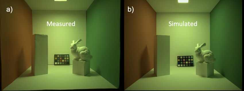
pect of the simulation with real data. The work we describe here is The Cornell box
a further validation of the image systems simulations. In this case, The first step in our simulations is to represent the 3D geom-
we construct a Cornell Box, a 3D scene designed to demonstrate etry of the Cornell Box and its contents, as well as the positions
physically based ray tracing methods, and we compare predicted of the light sources and camera. This can be accomplished us-
and measured camera data. ing several available computer graphics programs for modeling
The Cornell box (Figure 1) was designed to include signif- 3D objects and scenes. For this project, we use Cinema 4D to
icant features found in complex natural scenes, such as surface- create a 3D model of the objects and to represent the position of
to-surface inter-reflections and high dynamic range [13]. The box the light and the camera. The 3D coordinates, mesh, texture maps
contains one small and one large rectangular object placed near and other object information were exported as a set of text files
the side walls of the box. The box is illuminated through a hole that can be read by PBRT [17].
at the top, so that some interior positions are illuminated directly The real Cornell box and the objects within the box were
and others are in shadow. The walls of the box are covered with built with wood, cut to the size specified by the model. The sur-
red and green paper, providing colorful indirect illumination of faces of the inside walls and the rectangular objects were painted
IS&T International Symposium on Electronic Imaging 2021 1
Imaging Sensors and Systems 2021 122-1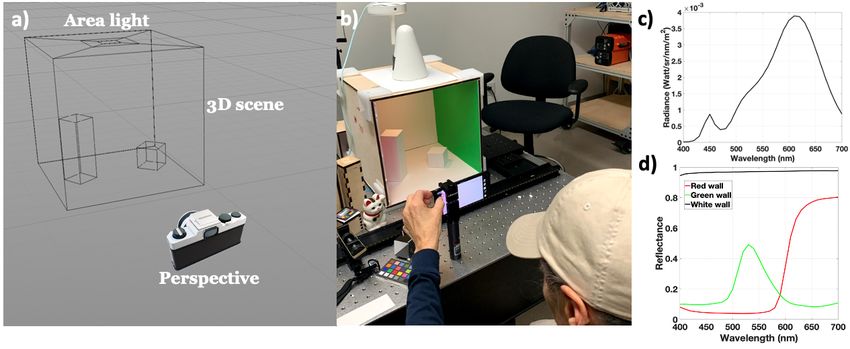
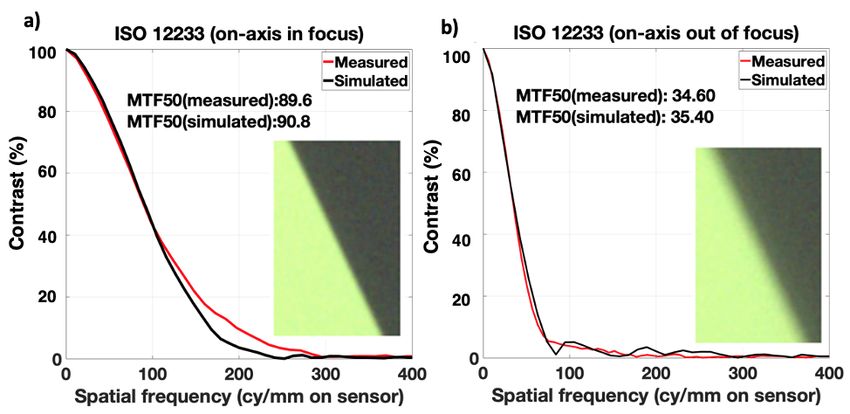
with white matte paint. The right and left walls were covered with ISO12233 analysis of the simulated and real camera images of
green and red matte paper, respectively. A hole was cut in the top the slanted edge target.
of the Cornell Box and covered with a diffuser; a light was placed We made the MTF comparison for targets at two different
on top of the diffuser. The spectral energy of the illuminant and distances. To model the defocus at different depths and field
spectral radiance of all surfaces within the Cornell box were mea- heights, we set the simulated defocus of a diffraction-limited lens.
sured with a PR670 spectroradiometer (See Figure 1cd). Figure 2 compares predicted and measured MTF curves when the
target is placed 50 cm away from the camera and is in focus (Fig-
ure 2a), and when the target is in the same position but the camera
is focussed 30 cm away (Figure 2b). The value of the Zernike
polynomial defocus term was 1.225 um for the in-focus plane and
3.5 um for the out-of-focus plane. Adjusting the defocus alone
brought the measured MTF and simulation into good agreement.
Sensor modelling
The simulated sensor irradiance image is converted to a sen-
sor response using ISETCam.
Figure 1. Virtual and Real Cornell box. a) Assets size, position of light
The Google Pixel 4a has a Sony IMX363 sensor, and many
source and camera perspectives are defined in Cinema 4D; b) Construction
of the sensor parameters can be obtained from published sensor
of a Cornell Box. c) Spectral power distribution of light source; d) Spectral
specifications (e.g., the pixel size fill factor, sensor size). We made
reflectance of the red and green surfaces.
empirical calibration measurements in our laboratory to verify a
subset of the published parameter values, specifically the spec-
We used an open-source and freely available Matlab toolbox tral quantum efficiency, analog gain, and various electronic noise
ISET3d [5, 8] to read the PBRT files exported from Cinema 4d sources (see Table 1 in the Appendix). We made these measure-
and to programmatically control critical scene properties, includ- ments using calibration equipment (PhotoResearch PR670 spec-
ing the object positions, surface reflectance, and illuminant spec- troradiometer) and OpenCam, a free and opens-source software
tral energy. This spectral information is part of the material and program that controls camera gain and exposure duration, and re-
light descriptions that are used by the rendering software, PBRT trieves lightly processed (“raw”) sensor digital values.
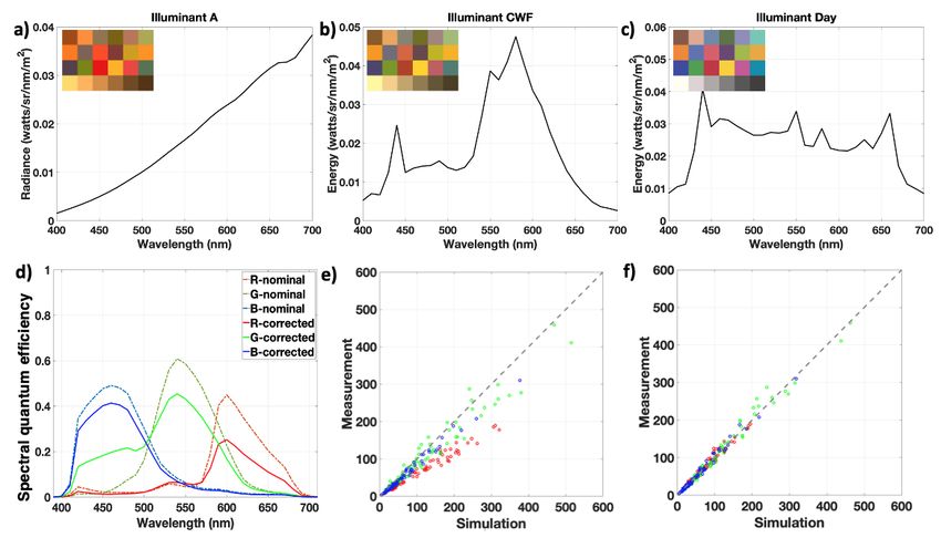
[17]. We modeled the surfaces as matte materials; the light was For example, to estimate the system sensor quantum effi-
modeled as an area light whose size matched the hole in the box ciency, we captured Google Pixel 4a camera images of a Mac-
made for the light. beth ColorChecker (MCC) illuminated by three different spectral
lights available in a Gretag Macbeth Light Box. We measured the
Optics modeling spectral radiance of each of the 24 color patches in the MCC and
PBRT calculates how light rays propagate from the light calculated the average R, G and B pixel values for the correspond-
source to surfaces in the scene, including the effects of surface ing color patches.
inter-reflections. PBRT also traces light rays through the optical
The dashed curves in Figure 3b show the spectral quantum
elements of a lens comprising multiple spherical or biconvex sur-
efficiency (QE) of the Google Pixel 4a based on published sensor
faces. The specific optical surfaces in the Google Pixel 4a, how-
datasheets. Figure 3c shows the measured RGB pixel values for
ever, are unknown to us. Thus, instead of using PBRT to model
each of the 24 color patches against the RGB pixel values pre-
the lens, we used an approximation. Specifically, we modeled
dicted by the product of the original sensor QE and the measured
a diffraction-limited lens with (1) the same f-number and focal
spectral radiance. The published spectral quantum efficiency of
length, (2) a small amount of depth-dependent defocus, and (3)
the Sony IMX363 does not include certain effects, such as opti-
empirically estimated lens shading.
cal and electrical crosstalk, or the channel gains. We calculated a
We introduced the defocus by modeling the wavefront
3x3 matrix, M, that transforms the original sensor QE curves and
emerging from the diffraction-limited lens using Zernicke poly-
nomial basis functions. A diffraction-limited lens has polynomial
weights of 1 followed by all zeros. We slightly blurred the im-
age by setting the defocus term (ANSI standard, j=4) to a positive
value [18]. We estimated the lens shading by measuring a uniform
image produced by an integrating sphere and fitting a low order
polynomial through the data.
In summary, we use PBRT to calculate the scene radiance.
We apply the lens blur and lens shading to calculate the irradiance
at the sensor.
We compared the spatial resolution of the simulated and
measured data by calculating the modulation transfer function
(MTF). To calculate the MTF, we simulated a scene of a slanted
edge target illuminated in the Cornell Box, and we captured Figure 2. Modulation transfer function (MTF) comparison. a) On-axis in-
Google Pixel 4a camera images of a real slanted edge target. focus MTF curves derived from images of the slanted bar. b) On-axis MTF
We used the ISO 12233 method to calculate MTFs based on an curves when lens is focused 20 cm in front of the slanted bar.
2 IS&T International Symposium on Electronic Imaging 2021
122-2 Imaging Sensors and Systems 2021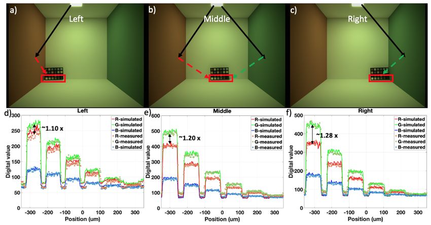
brings the predicted and measured RGB pixel values into better blur, chromatic properties, and noise, will match. We quantify
correspondence (see Figure 3f): the validity of the simulations by comparing small regions in the
measured sensor data with the simulated sensor data.
[r0 , g0 , b0 ] = [r, g, b]T M (1)
where r, g, and b are the vectors describing the published spectral Sensor digital values
quantum efficiency (QE) for red, green and blue channels (dashed The data in Figure 3f show that the sensor simulations pre-
lines, Figure 3d). The terms [r0 , g0 , b0 ] are the transformed QE dict the mean RGB digital values for the 24 color patches in the
vectors. The matrix M minimizes the least squared error between MCC target illuminated by 3 different lights. Here, we evalu-
measured and simulated sensor data for the 24 MCC color patches ate the accuracy of the digital values when the MCC color target
under the three different lights: is placed in a more complex environment that includes surface
inter-reflections. The simulated images in Figure 5a-c show the
0.532 0 0 Cornell box with an MCC target placed at three different posi-
M = 0.06 0.70 0 tions. We measured images that are very similar to these three
0 0.36 0.84 simulated images. In both cases, we expect that the digital values
The diagonal entries of M are a gain change in each of the measured from the MCC will vary as its position changes from
three channels; the off-diagonal entries represent crosstalk be- near the red wall (left) to near the green wall (right).
tween the channels. The transformed spectral QE data are the The graphs (Figures 5d-f) show the RGB digital values for a
solid curves in Figure 3c. These spectral QE curves produce a horizontal line of image pixels through the bottom row (gray se-
better match with the measured RGB values (compare Figure 3ef). ries) of the MCC. The solid lines show the simulated channels and
Hence we used the transformed curves in the simulations. the individual points show corresponding measurements. When
the MCC is near the red wall the R/G ratio is highest, decreasing
Validations as the MCC position shifts towards the green wall.
Figure 4 shows real and simulated raw Google Pixel 4a cam- The lowest pixel values - between the patches - are slightly
era images of a MCC target illuminated in the Cornell Box. The higher for the measured sensor image than the predicted camera
sensor data are formatted as Bayer color filter arrays. To simplify image. This difference occurs because the reflectance of the black
the comparison, we demosaicked the measured and simulated raw margins separating the color patches of the MCC is higher than
sensor image data using a bilinear interpolation. the simulated reflectance (which we set to zero). Within each of
the patches, the levels and the variance of the digital values are
Qualitative comparison similar when comparing the measured and simulated data. The
The simulated and measured images share many similarities. agreement between these two data sets confirms that the sensor
Both represent the high dynamic range of the scene: The pixels noise model is approximately accurate. We explore the noise
in the light source area on the top are saturated while the shadows characteristics quantitatively in the next section.
are simulated next to the cubes. Both camera images illustrate the
effect of light inter-reflections: The side surface of the cube on Sensor noise
the left is red due to the reflection from the left wall. Sensor pixel values start from a noise floor, rise linearly with
We do not expect that the measured and simulated sensor light intensity over a significant range, and then saturate as the
data can match on a pixel-by-pixel basis. Rather, we only ex- pixel well fills up. The signal measured at each pixel includes
pect that critical properties of the two sensor data sets, including both photon and electrical noise. In addition, there are variations
between pixels in their noise floor levels (DSNU) and photore-
sponse gain (PRNU). These noise sources make different contri-
butions depending on the mean signal level, and the combined
effects of the noise sources contribute to the standard deviation of
the digital values.
We selected three corresponding regions from the measured
and simulated sensor images where the mean values match (Fig-
ure 6ab), and compared the standard deviations in the measured
and simulated digital values. Figure 6c confirms that the mean
levels in the three selected regions match closely. Figure 6d shows
Figure 3. Sensor spectral quantum efficiency (QE). (a-c) Spectral energy
of the lights used to illuminate the MCC. d) Published (dashed lines) and
transformed (solid lines) spectral QE for the Sony IMX363 sensor. e) Scatter
plot comparing the predicted and simulated mean RGB values for 24 color
patches based on the published spectral QE. f) Scatter plot comparing pre-
dicted and simulated Mean RGB values based on the transformed spectral
QE curves. Figure 4. An example of measured and simulated images.
IS&T International Symposium on Electronic Imaging 2021 3
Imaging Sensors and Systems 2021 122-3
Figure 5. Analysis of sensor digital values. a-c): Simulated sensor images showing the MCC in different positions within the Cornell box. The arrows indicate
the strong indirect lighting from the two colored walls. The red boxes outline the gray series of the MCC. d-f) The digital values from a line through the gray series
of the simulated sensor data (solid) and measured sensor data (dots). The mean luminance of the simulated image was 21.5 cd/m2. To match the levels of the
simulated and measured data on the left and right, we multiplied the simulated data by 0.95 (right) and 0.75 (left). We believe the scaling is necessary because
we did not match the orientation of the MCC as we repositioned it against the back wall.

that the standard deviations of the three channels in each of the                     invariant wavefront model. When the design is known this ap-
three regions are similar. At the lower mean signal levels, the                       proximation is not necessary. We are developing methods to lift
standard deviations are equal. At the higher mean levels, the sim-                    this limitation through the use of black-box optics models.
ulated noise is slightly larger than the measured noise. The largest
difference between the observed and expected standard deviation
is about 2 digital values.

Discussion
      The simulated images are similar to the sensor data mea-
sured from these moderately complex scenes (Figure 4). The
simulation accounts for factors including object shape, surface
reflectance, lighting geometry and spectral power distribution, in-
terreflections, sensor spectral quantum efficiency, electronic noise
and optics. The simulations do not predict a point-by-point match,
but the mean signal and noise in corresponding regions agree to
an accuracy of a few percent. This level of agreement is similar
to the agreement between two cameras of the same model.
     There are several limitations of this work. The validations
are mainly confined to paraxial measurements and relatively uni-
form regions over the image. We plan additional evaluations to
predict data at large field heights, more extensive depth of field,
and higher dynamic range. There are at least two reasons why we
do not think it will be possible to achieve pixel-by-pixel matches
between the simulated and measured data: There will be minor                          Figure 6.    Sensor noise analysis. (a,b) We selected three regions in the
differences between the real materials and the simulations, and                       measured and simulated images (red squares) where the mean RGB values
some geometric differences will remain because we cannot per-                         of the measured and simulated sensor data were nearly equal. (c) The mean
fectly match the camera position between simulation and real-                         digital values for the nine values (RGB, 3 locations) are shown as a scatter
ity. Finally, because the design of lenses used in Pixel 4a was                       plot. (d) The standard deviations of the simulated and measured digital val-
unknown to us, we approximated the optics model with a shift-                         ues shown as a scatter plot.

                                                                                  4                      IS&T International Symposium on Electronic Imaging 2021
122-4                                                                                                                          Imaging Sensors and Systems 2021
There are many benefits of end-to-end image system sim-                     [9] Z. Liu, T. Lian, J. Farrell, and B. Wandell, “Soft prototyping camera
ulations. First, simulations can be performed prior to selecting                      designs for car detection based on a convolutional neural network,”
system components, making simulations a useful guide in system                        in Proceedings of the IEEE International Conference on Computer
design. Second, simulations enable an assessment of two designs                       Vision Workshops, 2019.
using the same, highly controlled, and yet complex input scenes.                 [10] J. Farrell, Z. Lyu, Z. Liu, H. Blasinski, Z. Xu, J. Rong, F. Xiao,
Repeatable evaluation with complex scenes can be nearly impos-                        and B. Wandell, “Soft-prototyping imaging systems for oral cancer
sible to achieve with real hardware components. Third, it is pos-                     screening,” Electronic Imaging, vol. 2020, no. 7, pp. 212–1–212–7,
sible to use simulation methods to create large data sets suitable                    2020.
for machine learning applications. In this way, it is possible to un-            [11] Z. Lyu, H. Jiang, F. Xiao, J. Rong, T. Zhang, B. Wandell, and
derstand whether hardware changes will have a significant impact                      J. Farrell, “Simulations of fluorescence imaging in the oral cavity,”
on the performance of systems intended for driving, robotics and                      bioRxiv, p. 2021.03.31.437770, Apr. 2021.
related machine learning applications.                                           [12] T. Lian, K. J. MacKenzie, D. H. Brainard, N. P. Cottaris, and B. A.
      We are using end-to-end image systems simulations meth-                         Wandell, “Ray tracing 3D spectral scenes through human optics
ods for a wide range of applications. These include designing                         models,” J. Vis., vol. 19, no. 12, pp. 23–23, 2019.
and evaluating novel sensor designs for high dynamic range imag-                 [13] C. M. Goral, K. E. Torrance, D. P. Greenberg, and B. Battaile, “Mod-
ing [19], underwater imaging [20], autonomous driving [21] and                        eling the interaction of light between diffuse surfaces,” SIGGRAPH
fluorescence imaging [10, 11]. End-to-end image systems simu-                         Comput. Graph., vol. 18, pp. 213–222, Jan. 1984.
lations can accelerate innovation by reducing many of the time-                  [14] M. F. Cohen, D. P. Greenberg, D. S. Immel, and P. J. Brock, “An ef-
consuming and expensive steps in designing, building and evalu-                       ficient radiosity approach for realistic image synthesis,” IEEE Com-
ating image systems. We view the present work as a part of an                         put. Graph. Appl., vol. 6, pp. 26–35, Mar. 1986.
ongoing process of validating these simulations.                                 [15] G. W. Meyer, H. E. Rushmeier, M. F. Cohen, D. P. Greenberg, and
                                                                                      K. E. Torrance, “An experimental evaluation of computer graphics
Acknowledgements                                                                      imagery,” ACM Trans. Graph., vol. 5, pp. 30–50, Jan. 1986.
    We thank Guangxun Liao, Bonnie Tseng, Ricardo Motta,                         [16] Sumanta N. Pattanaik, James A. Ferwerda, Kenneth E. Torrance,
David Cardinal, Zhenyi Liu, Henryk Blasinski and Thomas                               and Donald Greenberg, “Validation of global illumination simula-
Goossens for useful discussions.                                                      tions through CCD camera measurements,” in Color and Imaging
                                                                                      Conference 1997, pp. 250–53, 1997.
Reproducibility                                                                  [17] M. Pharr, W. Jakob, and G. Humphreys, Physically Based Render-
     The suite of software tools (ISET3D, PBRT and ISET-                              ing: From Theory to Implementation. Morgan Kaufmann, Sept.
Cam) are open-source and freely available on GitHub (see                              2016.
https://github.com/ISET). Scripts to reproduce the figures in this               [18] Wikipedia, “Zernike polynomials — Wikipedia, the free en-
abstract are in that repository.                                                      cyclopedia.”       https://en.wikipedia.org/wiki/Zernike_
                                                                                      polynomials. [Online; accessed 09-May-2021].
References                                                                       [19] H. Jiang, Q. Tian, J. Farrell, and B. A. Wandell, “Learning the im-
 [1] J. E. Farrell, P. B. Catrysse, and B. A. Wandell, “Digital camera                age processing pipeline,” IEEE Transactions on Image Processing,
     simulation,” Appl. Opt., vol. 51, pp. A80–90, Feb. 2012.                         vol. 26, no. 10, pp. 5032–5042, 2017.
 [2] J. E. Farrell, F. Xiao, P. B. Catrysse, and B. A. Wandell, “A sim-          [20] H. Blasinski and J. Farrell, “Computational multispectral flash,” in
     ulation tool for evaluating digital camera image quality,” in Image              2017 IEEE International Conference on Computational Photogra-
     Quality and System Performance, vol. 5294, pp. 124–131, Interna-                 phy (ICCP), pp. 1–10, May 2017.
     tional Society for Optics and Photonics, Dec. 2003.                         [21] Z. Liu, J. Farrell, and B. A. Wandell, “ISETAuto: Detecting ve-
 [3] J. Farrell, M. Okincha, and M. Parmar, “Sensor calibration and sim-              hicles with depth and radiance information,” IEEE Access, vol. 9,
     ulation,” in Digital Photography IV, vol. 6817, p. 68170R, Interna-              pp. 41799–41808, 2021.
     tional Society for Optics and Photonics, Mar. 2008.
 [4] J. Chen, K. Venkataraman, D. Bakin, B. Rodricks, R. Gravelle,               Author Biography
     P. Rao, and Y. Ni, “Digital camera imaging system simulation,”                    Zheng Lyu is a PhD candidate in the Department of Electrical En-
     IEEE Trans. Electron Devices, vol. 56, pp. 2496–2505, Nov. 2009.            gineering at Stanford University.
 [5] Z. Liu, M. Shen, J. Zhang, S. Liu, H. Blasinski, T. Lian, and B. Wan-             Krithin Kripakaran, De Anza College and a research assistant at
     dell, “A system for generating complex physically accurate sensor           Stanford University.
     images for automotive applications,” arXiv, p. 1902.04258, Feb.                   Max Furth, a student at Brighton College, England.
     2019.                                                                             Eric Tang, a student at Gunn High School, Palo Alto, CA.
 [6] T. Lian, J. Farrell, and B. Wandell, “Image systems simulation for                Brian A. Wandell is the Isaac and Madeline Stein Family Professor
     360 deg camera rigs,” Electronic Imaging, vol. 2018, pp. 353–1–             in the Stanford Psychology Department and a faculty member, by courtesy,
     353–5, Jan. 2018.                                                           of Electrical Engineering, Ophthalmology, and the Graduate School of
 [7] H. Blasinski, T. Lian, and J. Farrell, “Underwater image systems            Education.
     simulation,” in Imaging and Applied Optics 2017 (3D, AIO, COSI,                   Joyce Farrell is the Executive Director of the Stanford Center for
     IS, MATH, pcAOP), Optical Society of America, June 2017.                    Image Systems Engineering and a Senior Research Associate in the De-
 [8] H. Blasinski, J. Farrell, T. Lian, Z. Liu, and B. Wandell, “Optimiz-        partment of Electrical Engineering at Stanford University.
     ing image acquisition systems for autonomous driving,” Electronic
     Imaging, vol. 2018, no. 5, pp. 161–1–161–7, 2018.

IS&T International Symposium on Electronic Imaging 2021                      5
Imaging Sensors and Systems 2021                                                                                                                        122-5
Appendix
Table1. Sony IMX363 sensor specification.

 Properties         Parameters              Values(units)
                    Pixel Size              [1.4, 1.4] (µm)
 Geometric
                    Fill Factor             100 (%)
                    Well Capacity           6000 (e− )
                    Voltage Swing           0.4591 (volts)
                    Conversion Gain         7.65 × 10⁻⁵ (volts/e− )
 Electronics
                    Analog Gain             1
                    Analog Offset           0 (mV)
                    Quantization            12 (bit)
                    Method
                    DSNU                    0.64 (mV)
 Noise Sources      PRNU                    0.7 (%)
 @Analog gain=1     Dark Voltage            0 (mV/sec)
                    Read Noise              5 (mV)

                                                                  6   IS&T International Symposium on Electronic Imaging 2021
122-6                                                                                       Imaging Sensors and Systems 2021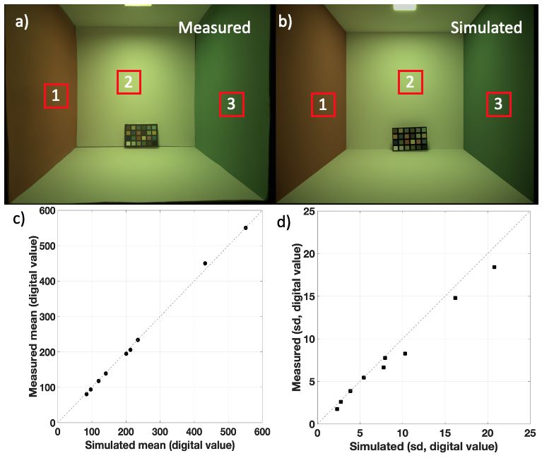
JOIN US AT THE NEXT EI!

 IS&T International Symposium on

 Electronic Imaging
 SCIENCE AND TECHNOLOGY

Imaging across applications . . . Where industry and academia meet!

• SHORT COURSES • EXHIBITS • DEMONSTRATION SESSION • PLENARY TALKS •
• INTERACTIVE PAPER SESSION • SPECIAL EVENTS • TECHNICAL SESSIONS •

                  www.electronicimaging.org
                                                             imaging.org
You can also read