GENERATIVE ADVERSARIAL NETWORK FOR MARKET HOURLY DISCRIMINATION - MUNICH PERSONAL REPEC ARCHIVE
←
→
Page content transcription
If your browser does not render page correctly, please read the page content below
Munich Personal RePEc Archive

Generative Adversarial Network for
Market Hourly Discrimination

Grilli, Luca and Santoro, Domenico

24 April 2020

Online at https://mpra.ub.uni-muenchen.de/99846/
MPRA Paper No. 99846, posted 24 Apr 2020 16:04 UTC
Generative Adversarial Network for Market Hourly

                                            Discrimination

                                   Luca Grilli✯ Domenico Santoro✯

                                                     Abstract

           In this paper, we consider 2 types of instruments traded on the markets, stocks and cryp-

       tocurrencies. In particular, stocks are traded in a market subject to opening hours, while
       cryptocurrencies are traded in a 24-hour market. What we want to demonstrate through the

       use of a particular type of generative neural network is that the instruments of the non-timetable
       market have a different amount of information, and are therefore more suitable for forecasting.

       In particular, through the use of real data we will demonstrate how there are also stocks subject
       to the same rules as cryptocurrencies.

        Keywords Neural Network · Price Forecasting · Cryptocurrencies · Market Hours ·
        Generative Model

        JEL classification C45 · E37 · F17 · G17

        Mathematics Subject Classification (2000) 91G80 · 62M45 · 91G60 · 97R40

   ✯ Università degli Studi di Foggia, Dipartimento di Economia, Management e Territorio, Via Da Zara, 11, I-71121

Foggia, Italy
Corresponding author: Luca Grilli, luca.grilli@unifg.it

                                                          1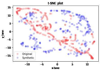
1    Introduction

The time series analysis has always attracted the attention of the academic world, in particular
by focusing on predicting the future values of these series. Financial time series are an optimal
candidate for such an analysis. These series base their assumptions on the random walk, a concept
introduced by Bachelier [15] in 1900 and since then remained a central pivot in the theory of time
series. Based on random walk theory, Kendall [9] assumed that the movement of stock prices was
random while Cootner [10] defined how the movement of stock prices could not be explained in
detail but was better approximated by the Brownian motion. Traditionally the best practice was
to focus on logarithmic returns, bringing the advantage of linking statistical analysis with financial
theory. Fama [4] introduced in his EMH theory (Efficient Market Hypothesis) the idea that his-
torical prices cannot be used to make predictions since all information is contained in the current
price. However LeRoy [7] showed that the mere concentration on yields was unjustified, defining
the stock markets inefficient. It was Taylor [13] who proposed an alternative model to the random
walk, developing a price trend model: he gave much empirical evidence that the price trend model
was important in analyzing prices on futures markets.
From an econometric point of view, Box et al. [21] introduced power transformations to statistical
models, also applying them to time series; in particular, they suggested using a power transforma-
tion to obtain an adequate Autoregressive Moving Average model (ARMA). On this basis Hamilton
[3] gave a formal (mathematically) definition of this model. Several evolutions followed this pattern,
like that Autoregressive Integrate Moving Average (ARIMA) and Seasonal Autoregressive Integrated
Moving Average (SARIMA).
Recently, thanks to the development of artificial neural networks (ANNs) and their ability to non-
linear modeling [22] there has been a strong interest in the application of these methods to time
series prediction. Foster et al. [23] were among the first to compare the use of neural networks
as function approximators with the use of the same networks to optimally combine the classically
used regression methods, highlighting how the use of networks to combine forecasting techniques
has led to performance improvements; Refenes et al. [20] proposed the use of a neural network

                                                  2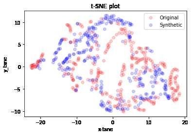
system for forecasting exchange rates via a feedforward network, which despite being correct for
66% had difficulty predicting any turning points; Sharda et al. [24] developed a comparison between
the prediction made via neural networks and the Box-Jenkins model, on the basis of which they
verified that for time series with long memory neural networks perform better than the forecast
while for time series with short memory the networks outperform the prevision.
The development of the financial time series forecasting has intensified mainly thanks to the new
techniques [2] of Machine Learning (ML) and Deep Learning (DL). As for ML techniques, Ko-
valerchuk et al. [1] have used models such as Evolutionary Computations (ECs) and Genetic
Programming (GCs); Li et al. [31] have developed a model for forecasting the stock price via ANN;
Mittermayer et al. [19] compared different text mining techniques for extracting market response
to improve prediction and Mitra et al. [17] have focused their attention on studying the news for
predicting anomalous returns in trading strategies. As for the DL techniques, especially in the last
10 years increasingly complex architectures are being used such as Liu et al. [26] who use a CNN
+ LSTM for strategic analysis in financial markets or like Zhang et al. [18] who use an SFM to
predict stock prices by extracting different types of patterns.
In this paper, we want to forecast problem related to financial market hours. Many of the stock
markets are subject to certain opening and closing times. In these types of markets when news
spreads or events occur outside closing hours, price reactions will only occur after the new opening
of the market. The cryptocurrency market (and currencies in general), however, is not subject to
closing times: it is open 24 hours a day. In this type of market the ”opening” price of the new day
and the ”closing” price of the previous day are recorded in a midnight interval every day, creating
continuity in the historical price series; or this reason the recorded prices are the sum of the events
relating to 24 hours and therefore containing more information useful for forecasting. Our goal is
to verify through an appropriate neural network how this difference of ”information in prices” can
lead to imbalances in the forecast, in particular linked to the discriminative and predictive power
of the prices themselves. Some studies, such as that of Tang [32] and Gorr [16] have shown that
neural networks are capable of modeling seasonality and other factors such as trend and cyclicity

                                                  3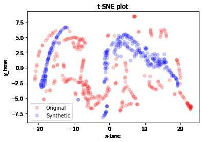
autonomously, therefore the different ”quantity of information” contained in the various types of
prices would seem to be the only cause that leads to forecast imbalances.
The paper structure is the following: in section 2 we analyzed the architecture of the main neural
networks used to make predictions in financial markets; in section 3 we have described the special
evolution of the GAN network used to extrapolate the characteristics of the different features in
the time series; finally in section 4 we have shown on which instruments the prediction is better
using real data.

2     Architectures of Neural Network

A neural network is a parallel computational model made up of artificial neurons. Each network is
made up of a series of neurons [27] with a set of inputs to which an output signal corresponds. The
neuron model was modified by Rosenblatt [8] who defined the perceptron as an entity with an input
and an output layer based on error minimization. Thanks to the study of associative memories and
the development of the Backpropagation algorithm by Rumelhart et al. [5] it paves the way for the
applications of feedforward networks, bringing to light the recurrent networks.
Neural networks are characterized by a learning algorithm that is a set of well-defined rules that
solve a learning problem and that allows you to adapt the free parameters of the network. The
learning algorithms can be of 3 types:

    ❼ Supervised learning, in this way the network learns to infer the relationship that binds input
      values with the relative output values;

    ❼ Unsupervised learning, where the network only has a set of input data and autonomously
      learns the mappings to be made;

    ❼ Semi-supervised learning, a mixed approach that combines a small amount of labeled values
      with a large amount of unlabeled values.

Neural networks can be classified in relation to the learning algorithm to be used, and in this regard

                                                  4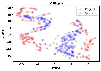
we distinguish between:
❼ Feedforward models, in which each layer has incoming connections from the previous and
outgoing to the next so that propagation occurs without cycles and transverse connections,
with training mainly supervised. For financial time series forecasting, a most widely used
model is that of CNN (Convolutional Neural Network). This type of network introduced by
LeCun et al. [30] was designed for image processing but it also found application in the
financial time series [6].
Figure 1: Architecture of a convolutional NN
This model, based on convolution, consists of a hierarchy of levels in which the intermediate
ones use local connections and the latter are fully-connected and operate as classifiers. The
key feature of this model is the presence of convolution and pooling levels, that aggregate the
information in the input volume generating a feature map of smaller dimensionality, so as to
guarantee invariance with respect to transformations and avoid the loss of information.
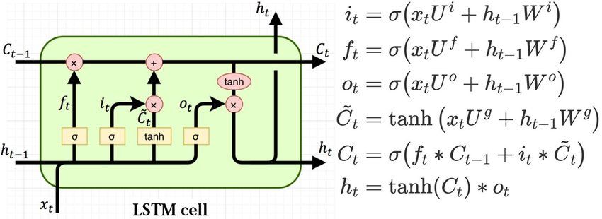
❼ Recurrent models (or feedback), cyclical so as to make the system dynamic. For financial
time series forecasting the most common RNN (Recurrent Neural Network) is the LSTM
(Long Short-Term Memory), introduced by Hochreiter et al. [25] in 1997. The characteristic
of this type of network is that at each step a level receives in addition to the input also the
output of the previous level, so that it can base decisions on history. However, since distant
memory tends to fade in base cells, the LSTM prevents this from happening through its
5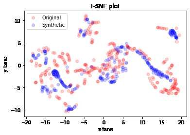
long-term memory.

              Figure 2: LSTM cells and equations that describe the gates [28]

  In this case, the state ht is a short-term memory state, while Ct is a long-term memory state:
  the cell learns what to forget from the past and what to extract and add from the current
  input.

❼ Generative models, used for input recognition and for pre-training of other models. The for-
  mulation of these models comes from an approach that has its roots in Bayes’ theorem, and
  they make sensorial hypotheses about the input in order to modify the parameters that char-
  acterize them. Learning is understood as the maximization of the likelihood of the data with
  respect to the generative model, which corresponds to discovering efficient ways of encoding
  the input information. For financial time series forecasting, the most used generative model
  is the GAN (Generative Adversarial Network) network, introduced in 2014 by Goodfellow et
  al. [11].

                                             6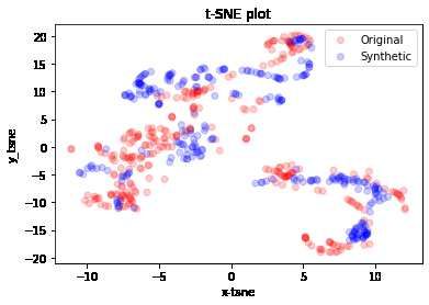
Figure 3: Generative adversarial network [12]
The GAN model consists of 2 networks: a generative network G that produces new data based
on a certain distribution pg and a discriminative network D that evaluates them, producing
the probability that x ∼ pdata where pdata is the distribution of training data. D and G play
the following two-player minimax game [11] with value function V (G, D):
min max V (D, G) = Ex∼pdata (x) [log D(x)] + Ez∼pz (z) [log(1 − D(G(z)))] (1)
G D
3 Methodology
One of the main problems in time series forecasting is the choice of the optimal variables to be taken
into consideration so that the neural network is able to capture their links and dynamics over time.
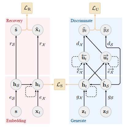
In particular, Yoon et al. [14] propose a new model, the Time-series Generative Adversarial Net-
works (TimeGAN) for generating realistic time-series data in various domains; which considers both
unsupervised adversarial loss and stepwise supervised loss and it uses original data as supervision.
According to the authors, this type of GAN is made up of 4 networks [14]: embedding function,
recovery function, sequence generator, and sequence discriminator. The autoencoding components
are trained jointly with the adversarial components such that TimeGAN simultaneously learns to
encode features, generate representations, and it iterates across time. Usually, GAN networks are
used (regarding financial time series) for the generation and therefore the replacement of any miss-
7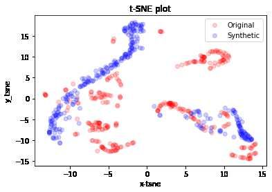
ing values (NaN), while in this case their main objective is to recreate a time series based on the
features used as input.

                                      Figure 4: TimeGAN [14]

   In this model, the generator is exposed to 2 types of inputs during training: the synthetic
embeddings in order to generate the next synthetic vector and the sequences of embeddings of
actual data to generate the next latent vector. In the first case, the gradient is computed on the
unsupervised loss, while in the second, the gradient is computed on the supervised loss. To highlight
generated results, Yoon et al. [14] have introduced a graphical measure for visualization, the t-SNE
[29] (so as to visualize how much the generated distribution looks like the original one) and 2 scores
(by optimizing a 2-layer LSTM):

   ❼ Discriminative score, it measures the error of a standardized classifier (RNN) in distinguishing
     between the real sequence and the one generated on the test set;

                                                  8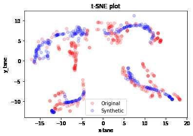
❼ Predictive score, represents the MAE (Mean Absolute Error) and measures the ability of
      synthetic data to predict next-step temporal vectors over each input sequence.

In addition, the t-SNE algorithm also returns the Kullback-Leibler Divergence (KL Divergence),
which is a measure of the difference between two probability distributions which indicates the
information lost when using a distribution (in this case the synthetic one) to approximate it another
(the original one).
What we want to demonstrate by using this network is that instruments listed on a market subject
to time constraints have a lower discriminative and predictive capacity than instruments present in
markets not subject to the same constraints. Financial instruments subject to timetables during the
continuous trading phase are representative of the information present in those hours, while what
occurs after closing cannot be captured by the price and will be recorded at least the following day
during the opening auction, which will lead to the price going up or down. On the other hand, for
instruments not subject to schedules, this problem does not arise since any type of event that may
have an effect on the price (whether it takes place day or night) will be recorded with an increase
or a decrease in the price itself. The exchanges give the possibility to carry out negotiations outside
the closing hours (Trading in Pre Market and After Hours) as in the case of Borsa Italiana in which
the Pre Auction phase is possible from 8:00 to 9:00 a.m. while After Hours trading is possible from
17:50 to 20:30 and NASDAQ where the Pre Market trading is possible from 4:00 to 9:30 a.m. (ET)
while After Hours trading is possible from 4:00 to 8:00 p.m. (ET), but certain time slots (which
could be key) remain uncovered. In this way, the ”amount of information” contained in each price
is therefore an essential element for time series forecasting.

                                                   9
3.1 Dataset
The empirical analysis was carried out on 2 types of instruments, stocks and cryptocurrencies.
Specifically these are
❼ Stocks1 :
1. GOOG (Alphabet Inc., Google), listed on NASDAQ;
2. AMZN (Amazon.com), listed on NASDAQ;
❼ Cryptocurrencies2 (all related to USD):
1. ETH (Ethereum Index);
2. BCH (Bitcoin Cash Index).
Prices are considered with a daily time frame over several years, from 20/12/2017 to 31/12/2019.
To test the discriminative and predictive ability of prices, the different datasets were divided into
2 types, the first with 5 features such as Open, Close (Last in the case of cryptocurrencies), High,
Low and Volume (generally indicated with the acronym OCHLV) while the second with only 2
features such as Open and Close/Last (indicated with the acronym OC).
3.2 Numerical examples
In this section, we will compare first from the graphic point of view and then through the scores
the capabilities of the different time series in terms of a difference in the amount of information.
This comparison is made especially by comparing the OCHLV datasets with the OC datasets for
the different instruments, so as to be able to test the basic idea. The graphical analysis will be
carried out by comparing the t-SNE plots, while the one based on the score will be carried out by
comparing the KL divergence, the discriminative score and the predictive score.
We can introduce the graphical analysis based on the t-SNE algorithm, in order to represent a
1 Source: finance.yahoo.com
2 Source: investing.com
10higher dimensional space in a two-dimensional scatter plot and to realize the adhesion between the
generated and synthetic data.
The first t-SNE analysis concerns the OCHLV dataset.
(a) Google (b) Ethereum
(c) Amazon (d) Bitcoin Cash
Figure 5: t-SNE analysis of synthetic data (blue) and original data (red) dataset OCHLV
From this analysis it is possible to highlight the potential of TimeGAN in the generation of data
and in particular in the cases represented in figures 5(b) and 5(d) (both cryptocurrencies) there is
a very precise adherence of the synthetic data to the originals. Obviously in this type of dataset
there is the presence of greater features which combined together allow the network to improve the
11forecast.
The second t-SNE analysis is based precisely on the OC dataset.
(a) Google (b) Ethereum
(c) Amazon (d) Bitcoin Cash
Figure 6: t-SNE analysis of synthetic data (blue) and original data (red) dataset OC
In this case at first glance it could seem like the synthetic data deviate from the original, however
with a more careful analysis it is possible to notice how in all cryptocurrencies the synthetic data
overlap the original data or imitate (albeit to a limited extent) their distribution, while in the
stocks’ case the distribution of the synthetic data is dispersive and not entirely consistent with the
distribution of the original data.
12The hypothesis we want to discuss is that the prices of cryptocurrencies have a greater amount of
information within them and have a greater discriminative and predictive power. This hypothesis
has been supported from the graphic point of view, but to leave no doubt we introduce the result
of the analysis based on the scores (Ds indicates the discriminative score while Ps the predictive
score) and on the KL divergence (DKL ).
Stocks Cryptocurrencies
OCHLV OC OCHLV OC
DKL = 0.477378 DKL = 0.390608 DKL = 0.372100 DKL = 0.261437
GOOG Ds = 0.1786 ± 0.0425 Ds = 0.1012 ± 0.0179 ETH Ds = 0.0712 ± 0.0006 Ds = 0.0758 ± 0.0503
Ps = 0.0773 ± 0.0018 Ps = 0.0517 ± 0.0016 Ps = 0.0425 ± 0.0012 Ps = 0.0412 ± 0.0087
DKL = 0.388102 DKL = 0.461293 DKL = 0.289605 DKL = 0.247001
AMZN Ds = 0.2238 ± 0.085 Ds = 0.1207 ± 0.0136 BCH Ds = 0.0804 ± 0.0272 Ds = 0.0862 ± 0.0735
Ps = 0.1208 ± 0.0019 Ps = 0.0662 ± 0.0237 Ps = 0.0259 ± 0.0002 Ps = 0.0307 ± 0.0058
Table 1: Score of both dataset (lower the better)
From the analysis of the values it is possible to notice how, especially in the case of the OC
dataset, the cryptocurrency scores are the lowest and therefore the most significant.
133.3 Outliers
A particular situation occurred when analyzing the stocks of Tesla Inc. (TSLA) listed on NASDAQ.
Despite being listed in a market subject to timetables, this analysis, both graphically and through
the scores through TimeGAN, resulted in having a price type ”loaded” with information, so much
so that it achieved almost better results than cryptocurrencies. In particular:
(a) OCHLV dataset (b) OC dataset
Figure 7: t-SNE analysis of TSLA stock on the different types of datasets
In both datasets the synthetic data reproduce the distribution of the original data very well.
The analysis of the scores shows the following results:
TSLA
OCHLV OC
DKL = 0.442472 DKL = 0.438634
Ds = 0.1139 ± 0.0374 Ds = 0.0434 ± 0.0060
Ps = 0.1131 ± 0.0100 Ps = 0.0402 ± 0.0006
Table 2: Score of TSLA in both dataset
In this case, especially in the OC dataset, it is noted that the price range has a very high
14discriminative and predictive power, even higher than that of cryptocurrencies. Thanks to this
”outlier” we can deduce that there are some instruments listed on stock exchanges subject to
timetables which despite the limitation are in any case ”completely absorbent” of the information
concerning the company. This situation could be linked, for example, to the hypothesis that negative
events never occurred outside the opening hours of the stock exchange or (in a less realistic but
still possible hypothesis) to the hypothesis that in the time range considered no external situations
occurred that could influence the price. In these cases, the use of this type of GAN can be a
”form of control” on prices, especially when these are to be used for forecasting. There may be
hidden elements that affect the price, however we can assume how the use of instrument whose
price has a ”large amount of information” could improve prediction compared to an opponent with
less information.
4 Conclusions
In this paper, we have shown how TimeGAN is able to highlight which securities have a time
series of prices ”loaded with information”. The prices of cryptocurrencies have shown to have a
much higher discriminatory and predictive power than stocks especially in the dataset made up
only of the opening and closing prices. Furthermore, in the complete dataset (OCHLV), the prices
with high discriminative power, combined with the other features, have made it possible to greatly
improve the adherence of the synthetic data to the original ones. From this analysis it emerged that
some stocks have the same discriminative and predictive power as cryptocurrencies; for this reason
(especially since the time series forecasting is carried out mainly on stocks) it seems appropriate to
screen, through this neural network, which are the optimal titles which combined with the different
features improve the forecast. The next step is to look for, if any, a relationship between this type
of stocks so as to limit the critical issues deriving from markets subject to timetables.
15References
[1] Kovalerchuk B. and Vityaev E. Data mining in finance: Advances in relational and hybrid
methods. Kluwer Academic Publishers, 2000.
[2] Sezer O. B., Gudelek M. U., and Ozbayoglu A. M. Financial time series forecasting with deep
learning: A systematic literature review: 2005-2019. arXiv:1191.13288, 2019.
[3] Hamilton J. D. Time series analysis. Princeton University Press, 1994.
[4] Fama E. Efficient capital markets: A review of theory and empirical work. Journal of Finance,
1970.
[5] Rumelhart D. E., Hinton G. E., and Williams R. J. Learning representation by back-
propagation errors. Nature, 1986.
[6] Chen J. F., Chen W. L., Huang C. P., Huang S. H., and Chen A. P. Financial time-series data
analysis using deep convolutional neural networks. IEEE 2016 7th International Conference
on Cloud Computing and Big Data, 2016.
[7] LeRot S. F. Efficient capital markets and martingales. Journal of Economic Literature, 1984.
[8] Rosenblatt F. The percepron: A probabilistic model for information storage and organization
in the brain. Psychological Review, 1958.
[9] Kendall M. G. The analysis of economic time series. part i: Prices. Journal of the Royal
Statistical Society, 1953.
[10] Cootner P. H. The Random Character of Stock Market Prices. MIT Press, 1964.
[11] Goodfellow I., Pouget-Abadie J., Mirza M., Xu B., Warde-Farley D., Ozair S., Courville A.,
and Bengio Y. Generative adversarial nets. Advances in Neural Information Processing System,
2014.
16[12] Hayes J., Melis L., Danezis G., and De Cristofato E. Logan: Evaluating privacy leakage of
generative models using generative adversarial networks. arXiv:1705.07763, 2017.
[13] Taylor S. J. Conjectured models for trends in financial prices, tests and forecast. Journal of
the Royal Statistical Society Series A, 1980.
[14] Yoon J., Jarrett D., and van der Schaar M. Time-series generative adversarial networks.
Advances in Neural Information Processing Systems 32 (NIPS 2019), 2019.
[15] Bachelier L. Théorie de la spéculatione. Ph.D. Thesis, 1900.
[16] Gorr W. L. Research prospective on neural network forecasting. International Journal of
Forecasting, 1994.
[17] Mitra L. and Mitra G. Applications of news analytics in finance: A review. The Handbook of
News Analytics in Finance, 2012.
[18] Zhang L., Aggarwal C., and Qi G. J. Stock price prediction via discovering multifrequency trad-
ing patterns. Proceedings of the 23rd ACM SIGKDD International Conference on Knowledge
Discovery and Data Mining, 2017.
[19] Mittelmayer M. and Knolmayer G. F. Text mining systems for market response to news: A
survey. 2006.
[20] Refenes A. N., Azema-Barac M., and Karoussos S. A. Currency exchange rate forecasting by
error backpropagation. Proceedings of the Twenty-Fifth Annual Hawaii International Confer-
ence on System Sciences, 1992.
[21] Box G. E. P. and Jenkins G. M. Time series analysis forecasting and control. San Francisco:
Holden-Day, 1976.
[22] Zhang G. P. Time series forecasting using a hybrid arima and neural network model. Neuro-
computing 50, 2003.
17[23] Foster W. R., Collopy F., and Ungar L. H. Neural network forecasting of short, noisy time
series. Computers and Chemical Engineering, 1992.
[24] Sharda R. and Patil R. B. Connectionist approach to time series prediction: An empirical test.
Journal of Intelligent Manufacturing, 1992.
[25] Hochreiter S. and Schmidhuber J. Long short-term memory. Neural Computation, 1997.
[26] Liu S., Zhang C., and Ma J. Cnn-lstm neural network model for quantitative strategy analysis
in stock markets. Neural Information Processing, 2017.
[27] McCullock W. S. and Pitts W. H. A logical calculus of the ideas immanent in nervous activity.
Bullettin of Mathematical Biophysics, 1943.
[28] Varsamopoulos S., Bertels K., and Almudever C. G. Designing neural network based decoders
for surface codes. arXiv preprint, 2018.
[29] van der Maaten L. and Hinton G. Visualizing data using t-sne. Journal of machine learning
research, 2008.
[30] LeCun Y., Bottou L., Bengio Y., and Haffner P. Gradient-based learning applied to document
recognition. Proceedings of the IEEE, 1998.
[31] Li Y. and Ma W. Applications of artificial neural networks in financial economics: A survey.
2010 International Symposium on Computational Intelligence and Design, 2010.
[32] Tang Z. and Almeida C. Fishwick P. A. Time series forecasting using neural networks vs.
box-jenkins methodology. Simulation, 1991.
18You can also read