COUNTING THE COSTS: CLIMATE CHANGE AND COASTAL FLOODING - Climate Council
←
→
Page content transcription
If your browser does not render page correctly, please read the page content below
COUNTING
THE COSTS:
CLIMATE
CHANGE
AND COASTAL
FLOODING
The Climate Council is an independent, crowd-funded organisation
providing quality information on climate change to the Australian public.

Climatecouncil.org.au
Authorship:
Will Steffen, John Hunter and Lesley Hughes
Published by the Climate Council of Australia Limited
ISBN:    978-0-9941623-0-4 (print)
         978-0-9941623-1-1(web)
© Climate Council of Australia Ltd 2014
This work is copyright the Climate Council of Australia Ltd. All material
contained in this work is copyright the Climate Council of Australia Ltd
except where a third party source is indicated.
Climate Council of Australia Ltd copyright material is licensed under
the Creative Commons Attribution 3.0 Australia License. To view a
copy of this license visit http://creativecommons.org.au
You are free to copy, communicate and adapt the Climate Council of
Australia Ltd copyright material so long as you attribute the Climate
Council of Australia Ltd and the authors in the following manner:
Counting the Costs: Climate Change and Coastal Flooding by Will
Steffen, John Hunter and Lesley Hughes (Climate Council of Australia).

Permission to use third party copyright content in this publication can
be sought from the relevant third party copyright owner/s.
This report is printed on 100% recycled paper.
Preface
     This is the 14th publication of the Climate   We are extremely grateful to our team
     Council. The Climate Council is an            of reviewers whose comments and
     independent, non-profit organisation,         suggestions improved the report.
     funded by donations from the public.          The reviewers were: Jon Barnett
     Our mission is to provide authoritative,      (University of Melbourne), Melanie
     expert information to the Australian          Bishop (Macquarie University), Bruce
     public on climate change.                     Thom (University of Sydney) and
                                                   Stefan Trueck (Macquarie University).
     Many Australians live on or near the
                                                   We thank CSIRO for reviewing the
     coast. The major population centres
                                                   accuracy and relevance of the science
     —Sydney, Melbourne, Brisbane, Perth,
                                                   underpinning the report. Their review is
     Adelaide, Hobart and Darwin—are all
                                                   not an endorsement of the conclusions
     port cities and much of the nation’s
                                                   drawn. We are also grateful to our expert
     critical infrastructure—transport,
                                                   contributors—Frank Jotzo (Australian
     commercial, residential, defence—is
                                                   National University) and Jan McDonald
     located along our coastlines. Virtually
                                                   (University of Tasmania)—for their
     all of this infrastructure has been
                                                   case studies (boxes) in this report.
     designed and built for a stable climate
                                                   We thank the Climate Council staff
     with known ranges of variability. But
                                                   for their many contributions to the
     the climate system is no longer stable.
                                                   production of this report.
     Sea level is rising and so are the risks
     for our coastal infrastructure.               The authors retain sole responsibility
                                                   for the content of the report.
     This report explores two of the most
     serious consequences of rising
     sea level—the large increase in the
     frequency of coastal inundation and
     the recession of ‘soft’ shorelines.
     Damage caused by increased coastal                          Professor Will Steffen
     inundation and recession poses a                            Climate Councillor
     massive financial burden due to damage
     and destruction of infrastructure.
     Coastal inundation and recession also
     have important implications for health
     and well-being, coastal ecosystems and
     communities. The report describes how                       Dr John Hunter
     scientific understanding of sea-level
     rise has improved significantly over
     the last decade, and we also explore the
     challenge of making better decisions
                                                                 Professor Lesley Hughes
     about future coastal development.
                                                                 Climate Councillor
     Finally, the report discusses the urgent
     need to stabilise the climate to reduce
     the level of risks from coastal flooding
     in the future.

Climatecouncil.org.au                                                                          Page i
COUNTING THE COSTS: CLIMATE CHANGE AND COASTAL FLOODING

             Introduction
             Australia is largely a coastal country.       rates of sea-level rise, as well as a better
             Much of our population lives on or near       understanding of regional variations
             the coast, and our six state capital cities   around the Australian coast. We can
             —Sydney, Melbourne, Brisbane, Perth,          assess the relative importance of various
             Adelaide and Hobart, as well as Darwin        factors, such as the warming of ocean
             in the Northern Territory—are all             water and the loss of ice from the polar
             port cities. In addition to the many          ice sheets, in driving sea-level rise.
             lifestyle amenities from living on the        Our knowledge of the behaviour of the
             coast, much of the nation’s critical          large polar ice sheets, such as those in
             infrastructure—transport, commercial,         Greenland and West Antarctica, has also
             residential, defence—is located along         improved, allowing better assessments
             our coastlines. Virtually all of this         of the risks from rapid and/or irreversible
             infrastructure has been designed and          loss of ice from these regions.
             built for a stable climate with known
                                                           Infrastructure that we are designing
             ranges of variability. But the climate
                                                           and building now should take climate
             system is no longer stable. Sea levels
                                                           change into account, but this is often
             are rising and so are the risks they
                                                           not the case. In addition to a solid
             pose for our coastal infrastructure.
                                                           scientific knowledge base, perceptions,
             The most immediate and serious                values, institutions, rules and other
             consequence of rising sea level is            social factors are crucially important
             the flooding of coastal areas through         in developing appropriate responses to
             both inundation and recession (see            climate‑related risks. An acceptance of
             Section 1). Coastal flooding creates          the reality of climate change and its risks
             many risks, including impacts on health       is essential, but much more is needed.
             and well‑being, damage to coastal             The challenge is to build effective
             ecosystems and disruption of people’s         approaches for dealing with the risks
             lives. In addition to these, the risks to     to existing infrastructure as well as
             coastal infrastructure – the major focus      making better decisions about future
             of this report - are potentially huge,        infrastructure development.
             particularly the economic losses due to
                                                           Ultimately, stabilising the climate is
             damage and destruction and the flow-on
                                                           necessary to reduce the level of risks
             effects to the economy more generally.
                                                           from coastal flooding. Rapid and deep
             Scientific understanding of sea-level rise    cuts in greenhouse gas emissions are
             has improved significantly over the last      critical here in Australia and around
             decade. We now have more reliable and         the world to stabilise the climate.
             accurate information on the observed

 Page ii                                                                   Climatecouncil.org.au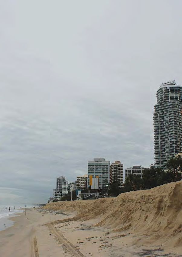
Contents
     Preface			                                                                                                                                                   i
     Introduction 		                                                                                                                                             ii
     Key findings		                                                                                                                                             iv

     1. Sea-level rise, coastal flooding and coastal infrastructure.......................... 1
     2. The science of sea-level rise ..........................................................................................................7
           2.1	Observations of sea‑level rise                                                                                                                    8
           2.2 Projections of future sea-level rise                                                                                                            12
           2.3	Increased probability of coastal flooding                                                                                                       16
           2.4	Other contributing factors to risks of sea-level rise                                                                                           20

     3. Counting the costs .................................................................................................................................21
           3.1	Infrastructure exposed to coastal flooding                                                                                                      23
           3.2	Observed economic costs of coastal flooding                                                                                                     25
           3.3 Projected costs of coastal flooding in future                                                                                                   28
           3.4	Other impacts of coastal flooding                                                                                                               34

     4. How can we deal with the risks?............................................................................................. 44
           4.1	The nature of the challenge                                                                                                                     45
           4.2 Do nothing: The head-in-the-sand approach                                                                                                       48
           4.3 Stabilise the climate system: Reducing greenhouse gas emissions                                                                                  51
           4.4 Be prepared: Adapting to the sea‑level rise we can’t avoid                                                                                      53

     5. The bottom line.......................................................................................................................................... 58
     References		60

Climatecouncil.org.au                                                                                                                                                  Page iii
COUNTING THE COSTS: CLIMATE CHANGE AND COASTAL FLOODING

             Key findings
             1. Sea level has already risen                      a business-as-usual approach to
                and continues to rise due                        burning fossil fuels would drive
                to climate change. Climate                       it towards the upper end.
                change exacerbates coastal                     ›› A sea-level rise of only 0.5 m
                flooding from a storm surge                       would, on average, mean that
                as the storm rides on higher                      a 1-in-a-100 year flood—a very
                sea levels.                                       rare event today—would occur
                ›› Climate change drives up sea                   every few months. It could also
                   level by warming the oceans and                involve a potential retreat of sandy
                   increasing the flow of ice from the            shorelines by 25 to 50 m.
                   land into the sea, for instance from        ›› Sydney is particularly vulnerable.
                   melting glaciers.                              It is likely that today’s 1-in-100 year
                ›› Over half the Australian coastline is          flood would occur every day or so
                   vulnerable to recession from rising            by 2100.
                   sea level, with 80% of the Victorian
                                                            3. Coastal flooding is a sleeping
                   coast and 62% of the Queensland
                                                               giant. If the threat of sea level
                   coast at risk.
                                                               rise is ignored, the projected
                ›› At both Fremantle and Sydney,               increases in economic
                   flooding events became three times          damage caused by coastal
                   more frequent during the 20th               flooding are massive.
                   century as a result of sea-level rise.
                                                               ›› More than $226 billion in
                ›› With just 10 cm of sea level rise              commercial, industrial, road and
                   the risks of coastal flooding                  rail, and residential assets around
                   roughly treble.                                Australian coasts are potentially
             2. Australia is highly vulnerable                    exposed to flooding and erosion
                to increasing coastal flooding                    hazards at a sea level rise of 1.1 m,
                because our cities, towns                         a high end, but quite plausible,
                and critical infrastructure are                   scenario for 2100.
                mainly located on the coast.                   ›› In Southeast Queensland—without
                Australia’s infrastructure                        adaptation—a current 1-in-100
                has been built for the climate                    year coastal flooding event risks
                of the 20th century and is                        damage to residential buildings
                unprepared for rising sea level.                  of around $1.1 billion. With a
                ›› Sea level is likely to increase                0.2 m rise in sea level, a similar
                   by 0.4 to 1.0 m through the 21st               flooding event would increase the
                   century. Strong action to reduce               damages to around $2 billion, and
                   greenhouse gas emissions would                 a 0.5 m rise in sea level would raise
                   constrain sea‑level rise towards               projected damages to $3.9 billion.
                   the lower end of that range, while

 Page iv                                                                    Climatecouncil.org.au
›› By 2050—without adaptation—the             ›› Australia’s multi-billion dollar
          losses from coastal flooding globally         tourism industry relies on
          are projected to rise to $US1 trillion        Australia’s beautiful sandy beaches,
          per year, about the size of the               from the Gold Coast to Fremantle
          entire Australian economy. By 2100            to Wine Glass Bay. Sandy beaches
          the losses from coastal flooding              are at risk from coastal erosion.
          are projected to be 0.3–9.3% of
                                                   5. Rising sea level is eroding
          global GDP per year. The high-end
                                                      the viability of coastal
          projection is a scenario for global
                                                      communities on islands
          economic collapse.
                                                      in the Torres Strait and the
     4. Rising sea levels pose risks                  Pacific, and in low‑lying
        for many of Australia’s species               areas of Asia, increasing
        and iconic natural places,                    the likelihood of migration
        such as Kakadu National Park                  and resettlement.
        and the Great Barrier Reef.                  ›› Several Torres Strait Island
       ›› Many ecosystems, like mangroves,              communities are situated on
          saltmarshes and seagrass beds,                extremely low-lying areas and
          may become trapped in a ‘coastal              already experience flooding during
          squeeze’ between rising sea levels            high tides. Building seawalls and
          and fixed landward barriers such as           raising houses can buy time, but in
          seawalls and urban development.               the long‑term, some communities
          Damaging these ecosystems                     may face relocation.
          has negative flow‑on effects to
                                                     ›› A sea-level rise of 0.5 to 2 m
          water quality, carbon storage
                                                        could displace 1.2 and 2.2 million
          and fisheries.
                                                        people from the Caribbean
       ›› Sea-level rise is increasing the              region and the Indian and Pacific
          salinity of coastal groundwater               Ocean islands, assuming that
          and pushing salty water further               no adaptation occurs.
          upstream in estuaries, affecting
                                                     ›› Globally, considerable displacement
          salt-sensitive plants and animals.
                                                        of people from the impacts
          Salt-water intrusion from rising
                                                        of climate change, including
          sea levels is contributing to the
                                                        increasing coastal flooding and
          loss of freshwater habitats in
                                                        erosion, is likely in coming decades.
          coastal regions such as Kakadu
                                                        Projections range from tens of
          National Park.
                                                        millions to 250 million people.
       ›› Some corals may not be able
          to keep up with periods of
          rapid sea‑level rise, leading to
          “drowning” of reefs.

Climatecouncil.org.au                                                                           Page v
COUNTING THE COSTS: CLIMATE CHANGE AND COASTAL FLOODING

             6. We need deep and urgent cuts
                in greenhouse gas emissions
                this decade and beyond if we
                are to avoid the most serious
                risks from rising sea levels
                and coastal flooding.
                ›› Stabilising the climate system
                   through deep and rapid reductions
                   in greenhouse gas emissions today
                   is the only way to significantly
                   reduce the level of risk that we face
                   from coastal flooding in the second
                   half of the century and beyond.
                ›› To prepare for the sea-level
                   rise that we can’t prevent is
                   also essential to lower the
                   risks of coastal flooding. This
                   requires a coordinated national
                   planning framework integrated
                   across federal, state and local
                   governments with clear allocation
                   of responsibilities.

             1.

 Page vi                                                   Climatecouncil.org.au
1.
Sea-level
rise, coastal
flooding
and coastal
infrastructure
Australians are very familiar        of seawater onto the coast. We
with the short-term, regular         are now experiencing another
variations in the level of the       driver of change to our coasts—
sea that occur on a daily basis      the global rise in sea levels
—the tides. We are also familiar     caused by the warming of the
with both longer-term variations     climate system. This sea-level
in the size of the tides that are    rise operates on much longer
related to the phases of the         timescales than the phenomena
moon and to short-term extreme       that we are used to experiencing,
flooding events that are caused      and will be with us for centuries.
by storm systems that drive a mass
COUNTING THE COSTS: CLIMATE CHANGE AND COASTAL FLOODING

               Sea-level rise affects the coast in two   waves, water currents and sediment
               distinct ways: by inundation, and by      supply and so is not determined solely
               coastal recession. Inundation is the      by changes in sea level.
               process by which the rise in sea level
               floods the land, without causing any
               change of the actual land surface.
               On the other hand, coastal recession
                                                         Over half the
               is the process by which “soft” (e.g.      Australian
               sandy or muddy) shorelines tend to
               be eroded landwards under a rising        coastline is
               sea level (Table 1). The latter process
               is complicated by the fact that coastal
                                                         vulnerable to
               recession (or the opposite effect,
               progradation, where the shoreline
                                                         erosion from
               migrates seawards) is affected by         rising sea level.
               several other processes such as

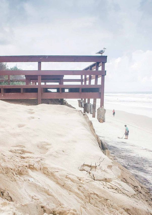
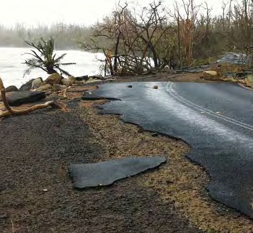
    Figure 1: An example of coastal recession at Broadbeach Queensland

 Page 2                                                                  Climatecouncil.org.au
01
Sea-level rise, coastal flooding and coastal infrastructure
Table 1: Fraction of coastline susceptible to recession under sea-level rise, defined
as shore composed of sand and mud, backed by soft sediment (so that recession is
largely unconstrained), and shore composed of soft rock. Based on DCC (2009).
State Total length of open Total length of Proportion of
coast, km vulnerable coast, km vulnerable coast (%)
Vic 2395 1915 80
NSW 2109 839 40
Qld 12,276 7551 62
NT 11,147 6990 63
WA 20,513 8237 40
SA 5876 3046 52
Tas 4995 2336 47
Aus 59,311 30,914 52
This report focuses primarily on the potential to restore themselves after
infrastructure, which is defined as the an erosion event—for example, after a
basic physical structures and facilities large storm.
needed for the operation of a society.
The average recession of sandy
Australia’s infrastructure is mostly
shorelines under sea-level rise can be
concentrated in the coastal zone around
roughly estimated through the Bruun
centres of population (DCC 2009; Chen
rule (Zhang et al. 2004), which states
and McAneney 2006). In this report,
that, on average for every metre of sea-
infrastructure includes buildings
level rise, sandy shorelines recede by
(private, commercial, industrial and
50–100 metres. The Bruun rule operates
public buildings), community services
on the assumptions that without sea-
(e.g. police, fire and ambulance stations,
level rise, the beach would be in steady
hospitals and schools), transport (e.g.
state and that other physical conditions
roads, railways, ports and airports) and
(e.g., waves or currents) are unchanged.
essential services (e.g. facilities for water,
No simple rule exists for the movement
waste treatment and energy supply).
of shorelines of mud or soft rock,
Defence facilities (e.g. naval bases)
although sea-level rise still tends to make
are also built assets under threat from
such shorelines recede. Table 1 above
climate change and coastal flooding.
shows the total lengths of vulnerable
In addition to infrastructure, other coastline susceptible to recession under
features of coastal regions are vulnerable adverse conditions such as sea-level rise;
to coastal inundation and recession. The these are defined as all those composed
impact of shoreline recession on the of sand and mud, which are backed by
land values along the coast is a prime soft sediment (so that recession is largely
example. Shorelines composed of sand, unconstrained), and all those composed
mud and soft rock may recede under of soft rock. More than half of Australia’s
changing environmental conditions coastline, about 31,000 km, is potentially
such as sea-level rise. However, sandy vulnerable to recession.
shorelines are the only ones that have
Climatecouncil.org.au Page 3COUNTING THE COSTS: CLIMATE CHANGE AND COASTAL FLOODING
It is not only human infrastructure One of the most common
that is at risk from rising sea levels and misconceptions about sea-level rise is
coastal flooding. Large stretches of that its rate – currently about 3 mm per
Australia’s coasts that are vulnerable to year—is so slow that it is not important
sea-level rise include coastal wetlands, in terms of impacts. By contrast, the
saltmarshes, mudflats, mangroves, impacts of extreme weather events,
seagrass beds, rocky shores and sandy such as heatwaves, extreme rainfall,
beaches. These provide important bushfires, are immediate and often very
habitats for many species, including serious. Similarly, sea-level rise is often
commercially and recreationally experienced via extreme inundation
important fish and shellfish. These or recession events.
ecosystems provide many additional
The immediate trigger of a high sea‑level
services, including protection from
event is often a combination of a high
erosion and storms, filtration of water
tide and storm surge (a “storm tide” is
and stabilisation of sediments (Spalding
the sum of a storm surge and tide). The
et al. 2014). The sediments within these
latter is a short-term rise in sea level
habitats also play a very important role
driven by strong winds and/or reduced
in carbon sequestration (“blue carbon”),
atmospheric pressure. Around northern
contributing about half of the total
Australia, storm surges are often driven
carbon burial in the oceans (Duarte
by tropical cyclones while intense low
et al. 2005).
pressure systems can also lead to storm
Many of these habitats are already in surges along our non-tropical coasts.
serious decline due to human impacts, For example, Cyclone Yasi caused a
and climate change is posing multiple large storm surge that contributed to
new threats. As sea levels rise, low‑lying extensive coastal flooding in north
habitats will become increasingly Queensland. Storm surges can extend
inundated. In some cases, species for hundreds of kilometres along a coast
and habitats will be able to adjust by and the area of flooding can extend
moving landwards but this will not be several kilometres inland in particularly
possible if the terrain is very steep, or low-lying areas. Other factors, such as
if human development is a barrier— human modification of the coastline,
the “coastal squeeze”. also influence the severity of the impacts
of a storm surge.
Tourism, one of Australia’s most
important income earners, is also As illustrated in Figure 2, the most
vulnerable. Our spectacular coastline direct link between coastal flooding and
and natural marine habitats are climate change is based on the fact that
central attractions for domestic and storm surges are now occurring on base
international visitors. Rising sea levels sea levels that have already risen and are
and increased coastal flooding pose continuing to rise. Storm surges are thus
great risks to the maintenance of our becoming more damaging as they are
beaches and the attractiveness and able to penetrate further inland.
access of many of our prime natural
When the weather system that drives the
tourist attractions.
storm surge—a tropical cyclone, large
Page 4 Climatecouncil.org.au01
Sea-level rise, coastal flooding and coastal infrastructure
Figure 2: Climate change exacerbates the effects of a storm surge increasing the base
sea level (Climate Commission 2013a).
storm or intense low pressure system— and the consequences that result. Both
also brings heavy rainfall to the coastal contributing factors are important. For
area, a “double whammy” flooding event example, an increase in the frequency
may occur as water comes from both of flooding events will obviously
the ocean (as described above) and from increase the risk of damage, but as
the land. These events may become more infrastructure is built in vulnerable
more common in future as the sea level locations and its value increases, the
rises and the probability of heavy rainfall consequences of a flooding event of
events increases (IPCC 2013). the same magnitude that occurred
previously will become more costly,
In this report we take a risk-based
thus also raising the risk.
approach to assessing the link between
climate change and coastal flooding The next section of this report examines
and adopt the simple relationship the changes that are occurring in the
shown in Figure 3 (an interpretation physical part of the equation—the
of the ISO standard definition) to assess observed rate of sea-level rise globally,
changes in risk. the regional variations in sea-level rise
around Australia, the factors that are
Risk is defined as the combination of the
driving the observed rise in sea level, and
likelihood that (or frequency with which)
the projected further rises in sea level to
an extreme flooding event will occur
Climatecouncil.org.au Page 5COUNTING THE COSTS: CLIMATE CHANGE AND COASTAL FLOODING
Figure 3: A diagram based on an interpretation of the ISO standard definition of risk
used in Australia and New Zealand (AS/NZS ISO 31000:2009).
Likelihood Consequence
(frequency, (impacts,
probability) damages)
Risk
the end of the century. Importantly, this to deal with the changing risk profile.
section also examines the changes in Because sea level is already rising as
the frequency with which high sea-level a result of climate change and will
events are likely to occur as the base sea continue to rise through this century
level rises. and beyond, denying climate change
and ignoring its consequences, or
Section 3 explores the other side of the
understanding the risks but failing to
risk equation—the consequences of
act, are not wise options. Adaptation
high sea-level events when they occur.
is essential to minimise the risk of
This section focuses strongly on the
high sea-level events, where the IPCC
economic costs associated with flooding
defines “adaptation” as “…the process of
and erosion, especially in urban areas.
adjustment to actual or expected climate
We also consider the coastline itself
and its effects, in order to moderate
(“soft” coasts) and the loss of property,
harm or exploit beneficial opportunities”
as well as the consequences of coastal
(IPCC 2012). Stabilising the climate
flooding and erosion for tourism and
system through deep and rapid emission
natural ecosystems.
reductions is also essential, as it will
Section 4 puts the two components influence the rate at which sea level
of the risk equation together and rises this century and the ultimate level
examines the approaches we can take at which it is stabilised.
Page 6 Climatecouncil.org.au2. The science of sea-level rise There is strong evidence that the coast is actually the result of primary cause of the sea-level two processes. They are the rise observed during the past vertical motion (rise or fall) half‑century was the warming of of the sea surface itself and the atmosphere and oceans due to the vertical motion (rise or an increase in the concentration subsidence) of the land surface of greenhouse gases in the adjacent to the sea. This is called atmosphere (IPCC 2013). Sea level relative sea-level change and is is certain to rise further through the change that is measured by the rest of this century and a tide gauge. On the other hand, beyond, leading to large increases a satellite measures the motion in frequency of coastal flooding. of the sea surface relative to The effect of changes in sea the centre of the Earth (called level that we experience at the a geocentric measurement).
COUNTING THE COSTS: CLIMATE CHANGE AND COASTAL FLOODING

             Relative sea-level change is the more       has provided scientific-quality sea level
             important measurement in terms of           data at 15 locations around Australia
             assessing impacts on infrastructure,        (see Figure 5 for locations).
             property and ecosystems. In many
             parts of the world today, especially
             around some large cities located on         Global-average
             deltas, impacts are increased by local
             subsidence of the land, which causes        sea level has risen
             relative sea-level rise to be greater
             than geocentric sea-level rise.
                                                         by 17 cm over the
                                                         20th century.
             2.1 Observations of
                 sea‑level rise                          The most widely used continuous
                                                         satellite observations of sea level started
             Sea level is most commonly observed         in 1992 and provide coverage of the
             by instruments, such as tide-gauges         world’s oceans, except near the poles,
             located on the coastline (generally in      approximately every 10 days. The broad
             ports), or satellites that measure the      spatial coverage of satellite observations
             height of the sea surface over most         has been combined with the long
             of the world’s ocean, using a form          duration of tide-gauge measurements
             of radar. In addition, methods called       to provide long-term regional records
             proxy techniques are sometimes used,        of sea-level change commonly called
             primarily in cases where instrumental       sea-level reconstructions. Examples of
             records are not available. Coring in salt   the global-average sea level derived from
             marshes is a popular proxy technique        these reconstructions are shown in Figure
             for the estimation of sea-levels over the   4 (Rhein et al. 2013), which indicates an
             past few centuries.                         average rise of about 17 cm (1.7 mm/
             Long-term tide-gauge measurements           yr) over the 20th century. Over the past
             started around 1700 in Amsterdam (Pugh      two decades, satellite observations
             and Woodworth 2014) and around the          indicate a global-average rate of about
             middle of the 19th century in Australia     3.2 mm/yr (Pugh and Woodworth 2014).
             (Hunter et al. 2003; Matthäus 1972). The    It is not clear at present whether this
             longest near-continuous Australian          apparent increase represents a long-term
             records are from Fremantle (from 1897)      acceleration or simply a manifestation of
             and Fort Denison (Sydney; from 1886)        natural variability. However, using model
             (NOC 2014). There are now around 300        results, Church et al. (2013a) concluded
             Australian locations where tide gauges      that ‘the increased rate of rise since 1990
             have been, or are being, operated. The      is not part of a natural cycle but a direct
             primary purpose of these gauges has         response to increased radiative forcing
             been to aid port and survey operations,     (both anthropogenic and natural), which
             rather than for scientific studies of       will continue to grow with ongoing
             sea level. From 1990 to the present,        greenhouse gas emissions’.
             however, the Australian Baseline Sea        Long-term tide-gauge records and
             Level Monitoring Project (BoM 2014d)        cores from salt marshes indicate that

 Page 8                                                                 Climatecouncil.org.au
02
The science of sea-level rise
a significant acceleration in sea-level at Hillarys is related to subsidence of the
rise occurred towards the end of the surrounding land, believed to be due to
nineteenth century (Church et al. 2013b). groundwater extraction for the city of
Perth (Burgette et al. 2013).
Figure 5 shows the observed rate of
relative sea-level rise around Australia
from 1990–1993 (the period of installation
of the ABSLMP tide gauges) to June 2014 Average sea‑level
(BoM 2014d). The average rate is 5.6 ± 2.3
(sd) mm/yr; the lowest rate is 3.5 mm/yr
rise around
at Stony Point (Vic) and the largest is 10.0
mm/yr at Hillarys (WA). These rates are
Australia has
all higher than the global-average rate been close to the
since 1992 of about 3.2 mm/yr measured
by satellite, although southeastern
global average.
Australia is closest to the global average.
If adjustments are made to Australian
There are a number of reasons for the
tide-gauge observations to account for
differences between the global rate and
ENSO, glacial isostatic adjustment (GIA;
those measured around Australia. Firstly,
the effect on relative sea level of changes
regional variations in sea level cover a
in the Earth’s loading and gravitational
range of scales in time and space. Over
field caused by past changes in land ice)
long time scales, if one region of the
and atmospheric pressure, the mean
oceans warms faster than elsewhere,
sea-level rise over the periods 1966–2009
the rate of rise will tend to be larger in
and 1993–2009 was 2.1 and 3.1 mm/yr,
that region. Such changes in ocean
respectively, which compares well with
temperature are inextricably linked with
the global-average sea-level rise over the
long-term changes in wind, pressure
same periods of 2.0 mm/yr (from tide
and/or ocean currents. At shorter time
gauges) and 3.4 mm/yr (from satellites)
scales, ocean-wide phenomena such as
(White et al. 2014). Over these periods,
the El Niño-Southern Oscillation (ENSO)
the mean sea-level rise around Australia
cause sea level at many (especially
was therefore close to the global-average.
western and northwestern) locations
around Australia to fall during an El The above analysis shows that
Niño event (Church et al. 2006). Douglas unadjusted observations of present
(2001) showed that individual tide- regional sea-level rise around Australia
gauge records need to be at least 50–80 should be treated with caution when
years long to average out such temporal considering the likely future sea‑level
variability and yield robust estimates of rise. The most useful estimates of
long-term local sea-level change (the future sea-level rise (i.e. the rise
records used to derive the trends shown several decades or more hence) come
in Figure 5 are only about 20 years long). from climate projections provided
Secondly, the rates of rise shown in by computer models (see Section 2.3)
Figure 5 are relative rates and so may be rather than from simple extrapolation
significantly affected by land movement. of recent observations.
The high rate of sea-level rise observed
Climatecouncil.org.au Page 9COUNTING THE COSTS: CLIMATE CHANGE AND COASTAL FLOODING
Figure 4: Yearly average global mean sea level reconstructed from tide gauges (1880–
2010) by three different approaches (Jevrejeva et al., 2008; Church and White, 2011;
Ray and Douglas, 2011). All uncertainty bars are one standard error as reported by the
authors. Adapted from IPCC AR5 WGI, Chapter 3, Figure 3.13(a) (Rhein et al. 2013).
(a) (b)
200 70
Church & White, 2011 60
150 Tide gau
Jevrejeva et al., 2008
Altimeter
GMSL anomaly (mm)
GMSL anomaly (mm)
Ray & Douglas, 2011 50
100
40
50 30
20
0
10
-50
0
-100 -10
1880 1900 1920 1940 1960 1980 2000 1992 1994 1996 1998 200
Year
(c) (d)
100 15
Figure 5: Observed rate of relative sea-level rise at 15 sites around Australia Sea level (Altim
for the
80 period 1990–1993 to June 2014 in mm/yr (BoM 2014d).
Sea level Mass (GRACE)
10
Thermosteric component
GMSL anomaly (mm)
60 GMSL anomaly (mm)
DARWIN
5
GROOTE EYLANDT
40
BROOME 0
20 CAPE FERGUSON
0
ROSSLYN BAY
-5
AUSTRALIA
-20 -10
1970 1975 1980 1985 1990 1995 2000 2005 2010 2005 2006 2007 2
HILLARYS THEVENARD
Year
PORT KEMBLA
ESPERANCE
PORT STANVAC
LORNE
STONY POINT
10.0 PORTLAND
BURNIE
8.0 TASMANIA SPRING BAY
6.0
4.0
Page 10 Climatecouncil.org.au02
The science of sea-level rise
Box 1: Sea-level rise budget
It is important to understand the processes that cause sea-level change if we are
to predict future changes. One way in which scientists gain this understanding is
to construct a budget of sea-level change, which entails comparing the observed
change in sea level with our best estimates of the individual contributions to that
change. For the current rise in sea level, these contributions are:
(i) Thermal expansion of the ocean water—warm water is less dense than
cooler water, and therefore takes up more space
(ii) Flow of ice from the land into the sea, which adds to the total amount of
water in the ocean. This additional water comes from:
(a) glaciers and ice caps (more recently referred to as “glaciers” only)
(b) the Greenland Ice Sheet
(c) the Antarctic Ice Sheet
(iii) Flow of liquid water between the land and the sea. This water may be stored
above ground or as groundwater. For example, increased storage of water
in dams lowers the rate of sea-level rise.
Thermal expansion of the oceans is estimated from measurements of
temperature and salinity (saltiness) in the oceans. Flow of ice from the land
into the sea is estimated by conventional glaciological and remote-sensing
(i.e. satellite and aerial) techniques. The amount of water on land and in
groundwater is derived by estimating the total volumes of natural and artificial
freshwater bodies, and aquifers.
A major advance reported in the IPCC Fifth Assessment Report (AR5) (Church
et al. 2013b) is that scientists now have a better understanding of the relative
importance of the main factors that cause sea-level rise, and can track how
these factors have changed over time.
Figure 6(a) shows the individual contributions to sea-level rise (coloured lines)
and the observed sea-level rise from tide gauges (black). The dashed black line
shows the observed satellite record. Figure 6(b) shows the same observations in
black, and the sum of the budget terms in red, so that a direct comparison can be
made between global observations of sea-level rise and the sum of the individual
components that contribute to sea-level rise (Church et al. 2011).
Since about 1970, the observations accord with the sum of the individual budget
terms, indicating that we have a good understanding of the relative importance
of the contributing factors to sea-level rise and how their importance is changing
through time. Since 1972, thermal expansion has contributed about 45% to total
sea-level rise, glaciers and ice caps about 40% with the remainder being made up
from Greenland and Antarctica, which are partially offset by water stored on land
and groundwater. There has been a significant acceleration in the contribution
from Greenland since 2000.
Climatecouncil.org.au Page 11COUNTING THE COSTS: CLIMATE CHANGE AND COASTAL FLOODING
Box 1: Sea-level rise budget (continued)
Figure 6: The global sea-level budget from 1961 to 2008. (a): The individual
terms of the budget (coloured) lines and observations of sea-level rise (black
solid and dashed lines); (b) The sum of the budget terms (red line) and observed
sea-level rise (solid and dashed black lines). Shading around the solid black
lines and around the red line in part (b) show the ±one standard deviation
uncertainty range. After Church et al. (2011).
Since 1972 thermal 2.2 Projections of future
sea-level rise
expansion has
The amount that sea level rises in the
contributed about future will depend on the amount of
45% to total sea- greenhouse gases emitted into the
atmosphere. The most commonly used
level rise and the projections of likely regional and global
loss of ice from sea-level rise cover the 21st century,
which corresponds to the period of most
glaciers and ice interest to coastal planners (see Section
4.2). The projections are based on certain
caps about 40%. assumed trajectories of atmospheric
greenhouse gas concentrations; in the
IPCC AR5, these are called Representative
Concentration Pathways or RCPs (van
Vuuren 2011; Box 2).
Page 12 Climatecouncil.org.au02
The science of sea-level rise
Box 2: Pathways of future greenhouse gas concentrations
in the atmosphere
Projections of future changes in the climate system, such as global-average
air temperature or sea-level rise, require assumptions about the changes
in the concentration of greenhouse gases in the atmosphere through time.
Throughout its Fifth Assessment Report, the IPCC (2013) has used the concept
of Representative Concentration Pathways, or RCPs, to provide trajectories of
changes in the concentration of greenhouse gases in the atmosphere.
RCPs are related to the rate at which human activities are emitting greenhouse
gases to the atmosphere, but are rather different from the emission scenarios
that have been used previously. The RCPs also incorporate the rate at which
greenhouse gases are absorbed by the oceans and by the land, the so-called
carbon sinks. Currently these carbon sinks absorb slightly more than half of
human emissions of carbon dioxide. Unless there are significant changes in
the strength of these sinks, the concentration pathways, or RCPs, will generally
reflect the rate of emission of greenhouse gases to the atmosphere.
Two RCPs are considered in this report:
(a) RCP4.5: this is a mitigation pathway that stabilises greenhouse gases in
the atmosphere by 2100. However, the temperature at the end of the 21st
century is more likely than not to exceed 2°C relative to the latter half of
the nineteenth century.
(b) RCP8.5: this is a “business as usual” trajectory in which atmospheric
greenhouse gas concentrations continue to rise through the century.
This trajectory will result in global temperatures around 4°C at the end
of the 21st century relative to the latter half of the nineteenth century.
Through the rest of this report, we use the term “weak mitigation pathway” for
RCP4.5 and the term “business as usual pathway”, or “BAU pathway”, for RCP8.5.
The IPCC also used a stronger mitigation pathway, RCP2.6, in its Fifth
Assessment. Of the four pathways that the IPCC used, RCP2.6 most closely
resembles the budget approach, described in Section 4.3, which requires
rapid and deep cuts in greenhouse gas emissions to stabilise the climate at
a temperature rise of no more than 2°C above pre-industrial. We focus on
RCP4.5 and RCP8.5 in this report to highlight the very serious risks from
coastal flooding that we face if we do not take decisive and rapid action
to reduce greenhouse gas emissions.
Climatecouncil.org.au Page 13COUNTING THE COSTS: CLIMATE CHANGE AND COASTAL FLOODING
Figure 7 shows the projected global-
average sea level rise for the weak Sea level could
mitigation pathway (blue) and for
the BAU pathway (orange), relative to
rise between
1986–2005, as reported in the IPCC AR5 0.4–1.0 m
(Church et al. 2013b). For each projection,
the central black line is the median, over the rest
and the coloured band represents the
“likely range”. This range represents
of this century
the 5- to 95-percentile range of the
model projections, and was further
depending on
interpreted in the AR5 as being the how rapidly we
range within which future sea level
has a 66% likelihood of occurring. reduce emissions
of greenhouse
The amount gases.
that sea level One potentially large future contributor
rises in the future to sea level that that cannot yet be
well modelled is the West Antarctic
will depend on Ice Sheet, the destabilisation of which
could add a few tens of centimetres to
the amount of the 2100 projections in a worst-case
greenhouse scenario (Church et al. 2013b). Recent
observations of changes in the West
gases emitted Antarctic Ice Sheet (Joughin and Alley
2011; Joughin et al. 2014; Rignot et al.
into the 2014) suggest that there are legitimate
atmosphere. concerns about its long-term stability
through the rest of this century.
Based on Figure 7, the sea-level rise over Two important analyses of risks to
the 21st century is in the approximate Australia’s coast (DCC (2009) and DCCEE
range 0.4–0.7 m for the weak mitigation (2011), which are referred to in Section
pathway and 0.5–1.0 m for the BAU 3, assumed a ‘high end’ sea-level rise at
pathway. These ranges are relatively 2100 of 1.1 metre, based on projections
large—about the same magnitude as from the IPCC’s 2007 Fourth Assessment
the lower limit of the estimate. However, Report (AR4) and other research
as will be shown in Section 2.4, this suggesting that the AR4’s projections
uncertainty increases the amount that may have been underestimated. Although
we need to allow for sea-level rise; it is higher than the upper 95-percentile
certainly not an excuse for inaction. limits shown in Figure 7, this ‘high end’
projection is still highly plausible.
Page 14 Climatecouncil.org.au02
The science of sea-level rise
If the West Antarctic Ice Sheet is
destabilised, sea-level could rise
higher than currently expected.
A major advance in the IPCC AR5 was Best estimates (central values) of sea‑
the development of regional projections level projections for Australia from the
of relative sea level, including the effects IPCC AR5, over the period 2010–2100,
of thermal expansion of the oceans, for the weak mitigation and the BAU
addition of water to the oceans through pathways, are shown in Figures 8a and
the flow of ice from the land into the 9a, respectively. The locations shown
sea, changes in ocean dynamics, and in these figures are the sites of long
past and future changes in the Earth’s (greater than about 30 years) Australian
gravitational field and in the vertical tide-gauge records. These sites are
movement of the Earth’s crust due to representative of the major population
the flow of ice from the land into the centres. In addition, these tide-gauge
sea. These projections are therefore the records provide the basis for the
most appropriate ones for determining estimation of the increased probability
the effect of sea-level rise on the coast. of coastal flooding described in Section
It should be noted, however, that these 2.3. The ranges of projected sea-level
projections do not include tectonic rise at the tide-gauge locations shown
effects or local land motion due to are 0.45–0.53 m and 0.65–0.76 m for
processes such as subsidence caused the weak mitigation and BAU pathways,
by groundwater withdrawal, as occurs respectively. The rise is slightly larger on
at Hillarys, WA (see Section 2.1). the southeast, east and northwest coasts
of Australia.
Figure 7: Projected global-average sea-level rise for the weak mitigation (RCP4.5: blue)
and BAU (RCP8.5: orange) pathways, relative to the average for the 1986–2005 period.
Climatecouncil.org.au Page 15COUNTING THE COSTS: CLIMATE CHANGE AND COASTAL FLOODING
Without 2.3 Increased probability
of coastal flooding
significant The surface of the sea is never still. Apart
reduction of from the increases we are measuring as
emissions, sea- a result of increasing greenhouse gas
emissions, the surface is continually
level rise will likely affected by tides, storm surges and
variations over seasonal, annual and
be measured decadal cycles. A piece of infrastructure,
if located near the coast, may experience
in metres in the occasional flooding event as result of
coming centuries. these variations in sea level.
Sea-level rise after 2100 becomes
progressively less certain, both due to
The frequency of
uncertainties inherent in the models
and to a lack of knowledge of future
coastal flooding
emissions. However, Church et al. (2013b) events trebles for
reported the spread of model projections
of global-average sea-level rise (over only every 0.1 m of
a few models) for a “medium scenario”
(which is similar to the weak mitigation
sea-level rise.
pathway) of 0.26–1.09 m and 0.27–
Such flooding events generally occur
1.51 m for 2200 and 2300, respectively
when a storm surge coincides with a
(both relative to 1986–2005). They also
high tide (Figure 2), but other processes
considered a “high scenario” (which
may come into play that make the
is similar to the BAU pathway), which
flooding event higher or lower. Under
gave model spreads of 0.58–2.03 m
a long-term trend of rising sea level,
and 0.92–3.59 m, for 2200 and 2300,
the frequency of flooding events (at a
respectively. We could possibly see a
given infrastructure height) increases.
rise of 2 m by 2450 under the “medium
Church et al. (2006) showed that, at
scenario” and by 2200 under the “high
both Fremantle and Sydney, flooding
scenario”. Without significant mitigation
events of a given height increased their
of emissions, sea-level rise will likely be
frequency of occurrence by a factor of
measured in metres in coming centuries.
about three during the 20th century as a
Over longer time periods, sea-level result of sea-level rise.
rise could be significantly higher.
A rough “rule of thumb” is that the
During the Last Interglacial Period,
frequency of flooding events trebles
about 120,000 years ago, when global
for every 0.1 m of sea-level rise (Hunter
temperature was 1° to 2° C warmer than
2012). Therefore, for a 0.2 m rise, the
pre-industrial (which will more likely
frequency of flooding events increases
than not be exceeded even under the
by a factor of about 3x3 = 9; for a 0.3 m
weak mitigation pathway) the sea level
rise, the frequency of flooding events
reached at least 5 m higher than present
increases by a factor of about 3x3x3 = 27,
(Church et al. 2013b).
and so on. Therefore, a 0.5 m rise (for the
Page 16 Climatecouncil.org.au02
The science of sea-level rise
21st century this would represent a mid- piece of infrastructure was designed for a
range projection for the weak mitigation 1-in-100-year flooding event (a common
pathway and a projection at the lower design criteria), it would experience the
end of the range for the BAU pathway) same flood every few months after the
would increase the frequency of flooding sea level had risen 0.5 m.
events by about 250. This means that, if a
For a sea-level rise of only 0.5 m, flood
events that today might be expected
once every hundred years could occur
every few months in the future.
As noted in Section 2.2, projections the multiplying factor is 10,000, what
of sea-level rise entail significant is now a 1-in-100-year flooding event
uncertainty. The multiplying factor by is projected to occur every few days
which the average frequency of flooding by 2100. Table 2 shows the multiplying
events increases with sea-level rise factors and impacts for Australian cities
depends both on the best estimate of in 2100 based on the BAU pathway.
that rise and on its uncertainty (Hunter This shows that Sydney, Bundaberg
2012). Taking both these contributions and Hobart would experience today’s
into account, Figures 8b and 9b show 1-in-100-year flooding event every day
this multiplying factor over the period or so by the end of this century. Even
2010–2100. There are wide ranges of in Adelaide (the least vulnerable city
multiplying factors over the locations shown in Table 2), today’s 1-in-100-year
shown: 13 to >10,000 and 45 to >10,000 flooding event would occur every year or
for the weak mitigation and BAU so by 2100.
pathways, respectively. In cases where
Table 2: Showing expected multiplying factors and impacts for Australian cities in
2100 based on the BAU pathway.
City Multiplying Impact
factor
Sydney >10000 1-in-100-year event would happen every day or so
Bundaberg >10000 1-in-100-year event would happen every day or so
Townsville 1500 1-in-100-year event would happen every month or so
Darwin >10000 1-in-100-year event would happen every day or so
Port Hedland 580 1-in-100-year event would happen every few months
Fremantle 820 1-in-100-year event would happen every month or so
Adelaide 120 1-in-100-year event would happen every year or so
Hobart >10000 1-in-100-year event would happen every day or so
Melbourne 2100 1-in-100-year event would happen more than every month
Climatecouncil.org.au Page 17COUNTING THE COSTS: CLIMATE CHANGE AND COASTAL FLOODING
A “planning allowance” may be derived of allowances over the locations shown
by calculating how much a piece of are 0.48–0.66 m and 0.72–0.95 m for
infrastructure would need to be raised the weak mitigation and BAU pathways,
to keep the average frequency of respectively, which are 0.1–0.2 m above
flooding events the same in the future the central values of the projections
as it is now. Figures 8c and 9c show (Section 2.2 and Figures 8a and 9a); this
this planning allowance over the period increase results from uncertainties in the
2010–2100 for the weak mitigation and projections. The allowances are larger on
BAU pathways, respectively. The ranges the southeast and east coasts of Australia.
Figure 8: (a) best estimate (metres), (b) multiplying factor, and (c) allowance (metres) for
2100 relative to 2010 for the sea-level rise projections for the weak mitigation pathway
(RCP4.5).
(a) (c)
DARWIN DARWIN
TOWNSVILLE TOWNSVILLE
PORT HEDLAND PORT HEDLAND
AUSTRALIA BUNDABERG AUSTRALIA BUNDABERG
FREMANTLE FREMANTLE
SYDNEY SYDNEY
MELBOURNE MELBOURNE
ADELAIDE ADELAIDE
0.70 0.70
0.60 TASMANIA HOBART 0.60 TASMANIA HOBART
0.50 0.50
0.40 0.40
(b)
Table 3: Showing expected impact for
DARWIN different multiplying factors.
Multiplying Impact
TOWNSVILLE factor
PORT HEDLAND
10000 1-in-100-year event would
AUSTRALIA BUNDABERG happen every few days
1000 1-in-100-year event would
happen every month or so
FREMANTLE
SYDNEY
100 1-in-100-year event would
happen every year or so
MELBOURNE
ADELAIDE
>1000 10 1-in-100-year event would
happen every ten years or so
1000
TASMANIA HOBART
100
10
Page 18 Climatecouncil.org.au02
The science of sea-level rise
Figure 9: (a) best estimate (metres), (b) multiplying factor, and (c) allowance (metres) for 2100
relative to 2010 for the sea-level rise projections for the weak mitigation pathway (RCP4.5).
(a) (c)
DARWIN DARWIN
TOWNSVILLE TOWNSVILLE
PORT HEDLAND PORT HEDLAND
AUSTRALIA BUNDABERG AUSTRALIA BUNDABERG
FREMANTLE FREMANTLE
SYDNEY SYDNEY
MELBOURNE MELBOURNE
ADELAIDE ADELAIDE
0.90 0.90
0.80 TASMANIA HOBART 0.80 TASMANIA HOBART
0.70 0.70
0.60 0.60
(b)
DARWIN
TOWNSVILLE
PORT HEDLAND
AUSTRALIA BUNDABERG
FREMANTLE
SYDNEY
MELBOURNE
ADELAIDE
>1000
1000
TASMANIA HOBART
100
10
Climatecouncil.org.au Page 19COUNTING THE COSTS: CLIMATE CHANGE AND COASTAL FLOODING
2.4 Other contributing There is much debate about whether this
is a sufficient safety margin. For example,
factors to risks of infrastructure is often designed to last
sea-level rise 100 years and also to just withstand the
“one-in-one-hundred-year” extreme
Coasts are always at risk, even in the
event. However (paradoxical as it may
absence of climate change and sea-level
seem), simple statistics tells us that such
rise. Coasts are exposed to storm surges
infrastructure is more likely than not to
and waves, which can cause inundation
experience something at least as severe
of low-lying land and modifications
as the one-in-one-hundred-year event
to soft shorelines (i.e. those composed
during its 100-year lifetime—therefore
of sand, mud or soft rock). Of the
it is more likely than not to get flooded
soft shorelines, sandy shorelines are
at least once. In the Netherlands, where
probably the least vulnerable because,
flooding could be widespread and
even though they can suffer significant
disastrous, coastal design and planning
recession after a large storm (which
is based on the 1-in-10,000-year extreme
brings high waves and often a higher
event, such that the likelihood of flooding
mean water level), they generally
in any 100-year period would only be
“repair” during quieter times. However,
about 1% (or 1 in 100) (Kabat et al. 2009).
as indicated in Section 1, sea-level rise
may lead to an overall recession, which As noted in Section 2.1, local subsidence
often manifests itself as an inadequate of land increases the rate of relative
“repair” process after a major storm. sea-level rise, thereby increasing the
Muddy and soft-rock shorelines cannot vulnerability of the shoreline to flooding.
repair themselves in this way once they This effect is evident at several locations
are eroded as there is no corresponding around Australia and is generally
post-storm “repair” process. due to the extraction of groundwater
(e.g. Hillarys, see Section 2.1; Adelaide,
Coastal engineers and planners design
see Belperio, 1993) or the extraction
infrastructure to cope with events of a
of oil and gas (e.g., Gippsland, see
certain probability of occurrence. For
Freij‑Ayou et al. 2007).
example much of our infrastructure
has been designed to cope with a
“one‑in‑one-hundred-year” extreme
event, which relates to a water level or
wave height that is exceeded, on average,
once in 100 years. This is approximately
the same as the water level or wave
height that has a likelihood of 1%
(or 1 in 100) of occurring in any one year.
Page 20 Climatecouncil.org.au3. Counting the costs The potential costs of coastal infrastructure damage and the flooding can be estimated in a resulting insurance claims, whilst number of ways, including (i) others incorporate indirect costs, the value of infrastructure that such as the economic disruption is exposed to coastal flooding, from flooded businesses or cut both at current sea level and at roads, the losses of state’s tax levels projected for the future; income, or long-term declines in (ii) observed damages of coastal property value. Projected costs flooding events that have already can also vary depending on the occurred; and (iii) estimated factors considered in different damages of future coastal studies, such as the presumed flooding events at a projected extent of sea level rise or the local amount of sea-level rise. adaptive capacity of the area at Various methods are used risk. The discount rate employed to assess present and future in the study can also have a large damages to infrastructure. Some bearing on projected future costs studies focus specifically on direct of coastal flooding.
COUNTING THE COSTS: CLIMATE CHANGE AND COASTAL FLOODING
Page 22
Figure 10: Counting the costs of coastal flooding
COA THE C
$226
RISK RISK RISK
AT AT AT
STA OST
L FL S OF
OO
DIN
BILLION WORTH
OF $87 $72 $67 G
INFRASTRUCTURE BILLION BILLION BILLION
& HOMES AT RISK COMMERCIAL &
LIGHT INDUSTRIAL
HOMES
AT RISK
ROAD & RAIL
AT RISK
QLD
FROM COASTAL INUNDATION
BUILDINGS AT RISK
AT A SEA LEVEL RISE OF $11.3-$17 billion worth of commercial
1.1 METRES.
and light industrial buildings at risk
WA $9.7-$12.9 billion
CLOSE TO of roads at risk
250, $12.7-$18.1 billion
of commercial and light
NT
HOMES
industrial buildings at risk
$0.1 - $0.5 billion
of rail and tramways at risk
RISK! AT $8.7-$11.3
BILLION
OF ROADS AT RISK
NSW
NATIONAL INFRASTRUCTURE SA Up to 68,000
WITHIN 200 M OF
THE COASTLINE $22.6-$28.2 BILLION HOMES AT RISK!
OF COMMERCIAL & LIGHT INDUSTRIAL
BUILDINGS AT RISK
120 $0.6-$1.3 billion of
PORTS rail and tramways at risk
$0.6-$1.3 billion of
Climatecouncil.org.au
5 POWER rail and tramways at risk
STATIONS
VIC TAS
258 POLICE, FIRE & Up to 48,000 Up to 15,000
AMBULANCE STATIONS
HOMES AT RISK! HOMES AT RISK!
75 HOSPITALS &
HEALTH SERVICES Over $7 billion $0.6-$1.3 billion of
of roads at risk rail and tramways at risk
44 WATER AND
WASTE FACILITIES Data relates to infrastructure exposed to coastal inundation and shoreline recession at a sea level rise of 1.1 metres (high end scenario for 2100). The
replacement values are drawn from Geoscience Australia’s National Exposure Information System (NEXIS) database. Source: DCC 2009; DCCEE 2011.You can also read


