COVID-19 Mortality and Con-temporaneous Air Pollution 8609 2020
←
→
Page content transcription
If your browser does not render page correctly, please read the page content below
8609
                                                                   2020
                                                                   October 2020

COVID-19 Mortality and Con-
temporaneous Air Pollution
Wes Austin, Stefano Carattini, John Gomez Mahecha, Michael Pesko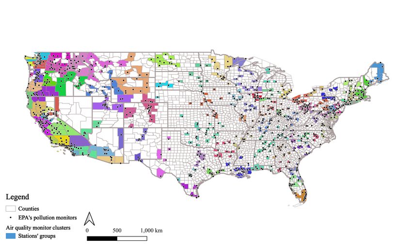
Impressum:

CESifo Working Papers
ISSN 2364-1428 (electronic version)
Publisher and distributor: Munich Society for the Promotion of Economic Research - CESifo
GmbH
The international platform of Ludwigs-Maximilians University’s Center for Economic Studies
and the ifo Institute
Poschingerstr. 5, 81679 Munich, Germany
Telephone +49 (0)89 2180-2740, Telefax +49 (0)89 2180-17845, email office@cesifo.de
Editor: Clemens Fuest
https://www.cesifo.org/en/wp
An electronic version of the paper may be downloaded
· from the SSRN website:       www.SSRN.com
· from the RePEc website:      www.RePEc.org
· from the CESifo website:     https://www.cesifo.org/en/wp
CESifo Working Paper No. 8609

         COVID-19 Mortality and Contemporaneous
                    Air Pollution
                                                  Abstract

We examine the relationship between contemporaneous fine particulate matter exposure and
COVID-19 morbidity and mortality using an instrumental variable approach based on wind
direction. Harnessing daily changes in county-level wind direction, we show that arguably
exogenous fluctuations in local air quality impact the rate of confirmed cases and deaths from
COVID-19. In our preferred high dimensional fixed effects specification with state-level policy
and social distancing controls, we find that a one μg/m3 increase in PM 2.5 increases the number
of confirmed cases by roughly 2% from the mean case rate in a county. These effects tend to
increase in magnitude over longer time horizons, being twice as large over
a 3-day period. Meanwhile, a one μg/m3 increase in PM 2.5 increases the same-day death rate by
3% from the mean. Our estimates are robust to a host of sensitivity tests. These results suggest
that air pollution plays an important role in mediating the severity of respiratory syndromes such
as COVID-19, for which progressive respiratory failure is the primary cause of death, and that
policy levers to improve air quality may lead to improvements in COVID-19 outcomes.
JEL-Codes: D620, I100, Q530.
Keywords: pollution, air quality, PM 2.5, COVID-19, health, mortality.

                   Wes Austin                                               Stefano Carattini
     Georgia State University / Atlanta / USA                    Georgia State University / Atlanta / USA
               gaustin4@gsu.edu                                            scarattini@gsu.edu
             John Gomez Mahecha                                              Michael Pesko
     Georgia State University / Atlanta / USA                    Georgia State University / Atlanta / USA
          jgomezmahecha1@gsu.edu                                            mpesko@gsu.edu

October 1, 2020
We thank Garth Heutel, Julie Hotchkiss, Daniel Kreisman, Rafael Lalive, James Marton, Givi Melkadze, Andrew
Schreiber, and Jonathan Smith for very helpful comments on a previous version of this paper. We also thank Unacast,
which provided the restricted access data on social distancing. While this paper was completed during his time at
Georgia State University, Austin is now affiliated with the National Center for Environmental Economics, U.S.
Environmental Protection Agency, Washington, DC. The views expressed in this paper are those of the authors and
do not necessarily reflect the views or policies of the U.S. Environmental Protection Agency (EPA). Carattini is also
affiliated with CESifo, the London School of Economics and Political Science, and the University of St. Gallen.
Carattini acknowledges support from the Grantham Foundation for the Protection of the Environment through the
Grantham Research Institute on Climate Change and the Environment and from the ESRC Centre for Climate Change
Economics and Policy as well as from the Swiss National Science Foundation, grant number PZ00P1 180006/1. The
usual disclaimer applies.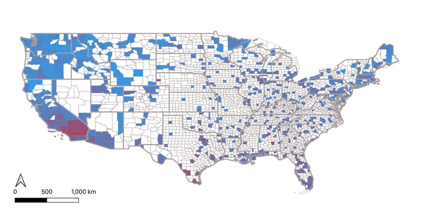
1     Introduction

As of September 2020, the 2019 novel Coronavirus has claimed over 870,000 lives globally. The total number

of confirmed Coronavirus cases has soared to 26.3 million. Since the start of the outbreak, unemployment

has increased and economic production decreased. Local governments are still defining the best strategies

for relaunching economic activity while minimizing the number of additional cases and deaths. A trade-off

exists between the speed at which economic activity is reopened and the risk of further cases and deaths.

    Our paper expands the policymakers’ toolkit by adding one more dimension to this trade-off: contem-

poraneous air pollution exposure. PM 2.5 has been associated with many of the co-morbidities that relate

to poor prognosis and death in COVID-19 patients, including lung and cardiovascular disease. PM 2.5

may therefore contribute to COVID-19 severity, thus increasing demand for testing, due to worsened symp-

toms, as well as mortality. We show that decreases in contemporaneous pollution are linked to decreases

in confirmed COVID-19 cases and mortality. Our empirical approach uses plausibly random daily changes

in wind direction to predict air pollution levels, providing quasi-experimental evidence of the effect of PM

2.5 exposure on COVID-19 outcomes (Luechinger, 2014; Deryugina et al., 2019; Anderson, 2020). In our

preferred high dimensional fixed effects specification with state-level policy and standard social distancing

controls from Unacast cell phone data, we show that a one µg/m3 increase in PM 2.5 increases the number

of confirmed cases by roughly 2% from the mean case rate in a county, where confirmed cases are likely to be

a measure for severe cases, given that in the case of COVID-19 many infected people do not show symptoms

(Day, 2020; Gandhi et al., 2020; Persico and Johnson, 2020). In absolute terms, this represents 0.7 additional

confirmed cases in a county on any given day. In the three-day period following a perturbation in air quality,

the relationship between fine particulate matter exposure and cases is over twice as large. Meanwhile, a one

µg/m3 increase in PM 2.5 increases the same-day death rate by 3% from the mean, or between 0.05 and 0.06

additional deaths per 100,000 individuals in a county. These results are in line with the medical literature,

which points to progressive respiratory failure as the primary cause of death from COVID-19 (Ackermann

et al., 2020), as well as an older literature in economics showing the immediacy of the relationship between

exposure to pollution and potential death (see Currie et al., 2014).

    Our paper contributes to several strands of literature. To start, we contribute to recent research that

associates past exposure to fine particulate matter with COVID-19 mortality (e.g., Wu et al., 2020). Our

paper expands our knowledge on the relationship between particulate matter and COVID-19 mortality in two

important ways. First, it focuses on current exposure to particulate matter. The contemporaneous dimension

is crucial because policymakers have control over current pollution levels but not over past exposure to air

pollution. Second, identification relies on plausibly exogenous variation in wind direction à la Deryugina

                                                      2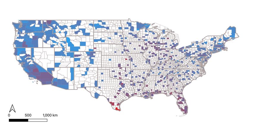
et al. (2019), which allows us to causally link particulate matter with COVID-19 outcomes in a nationwide

study for the United States, covering virtually all polluting sources. Hence, we generalize previous findings

showing that changes in air pollution from recent regulatory changes affecting Toxic Release Inventory sites

can have an impact on number of deaths and confirmed cases of COVID-19 (Persico and Johnson, 2020).

Further, our study contributes to a growing literature showing detrimental effects of air pollution on a wide

range of outcomes, such as infant mortality (e.g., Chay and Greenstone, 2003; Chay et al., 2003; Currie and

Neidell, 2005; Knittel et al., 2016), birth weight (e.g., Currie and Walker, 2011), dementia (e.g., Bishop et al.,

2018), contemporaneous and long-run education outcomes (e.g., Lavy et al., 2012; Sanders, 2012; Ebenstein

et al., 2016) and other measures of productivity (e.g., He et al., 2019). Among the many outcomes that have

been studied (see also Currie et al., 2014; EPA, 2019), non-infant mortality has been largely neglected, with

only a handful of studies covering it (such as Chay et al., 2003; Chen et al., 2013; Deschênes et al., 2017;

Deryugina et al., 2019). Our paper contributes to fill this gap. Further, it adds to the growing body of work

illustrating the short-term effect of pollution on health outcomes, including the relationship between days

of exposure to pollution and mortality (e.g., Arceo et al., 2016; Simeonova et al., 2018; Deryugina et al.,

2019; Anderson, 2020). Overall, we contribute to the literature on pollution and health by showing that

air pollution, and in particular fine particulate matter, also plays an important role in the management of

deadly infectious diseases such as COVID-19, whose impacts have dramatically affected many cohorts in

society, and that these effects emerge very rapidly. Finally, our study contributes to an emerging literature

on the economics of the COVID-19 pandemic, aiming at identifying the best possible responses to the current

emergency (see Brodeur et al., 2020 for a review). Compared to other studies in the literature, the approach

used in this paper has also the advantage of addressing potential measurement error in COVID-19 outcomes.

   Our findings have important policy implications. From the contemporaneous relationship between PM

2.5 and COVID-19 morbidity and mortality, it follows that keeping current pollution at low levels may have

an immediate payoff in that it may allow for fewer additional cases and deaths when reopening the economy.

Policymakers have a wide range of policy levers available to reach this goal, as discussed in Section 6.

   The remainder of the paper is organized as follows. Section 2 describes our data. Section 3 introduces our

empirical methods and identification strategy. Section 4 presents our main empirical results. Section 5 con-

firms these results based on a battery of robustness tests. Section 6 illustrates our main policy implications.

Section 7 concludes.

                                                        3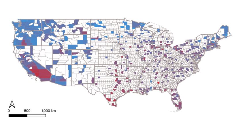
2     Data

This paper uses daily information about the COVID-19 outbreak, pollution levels, wind, and social distancing

behavior at the county level from January 22nd to August 15th . We also use state-level information on policies

adopted to curb the spread of the virus. Our data is limited to the contiguous United States and counties

with an EPA air quality monitoring station. In the following sections, we describe data sources and the

construction of the final database.

2.1     Coronavirus Cases and Deaths

The Johns Hopkins University Center for Systems Science and Engineering provides mortality and caseload

information for the study.1 It offers a web-based data repository available since January 22nd , developed for

researchers, public health authorities, and the general public to track the outbreak. The platform reports

raw daily caseload and death figures for each county in the United States and has arguably become the

standard source of data for cases and deaths in the growing COVID-19 literature. The number of cases

and deaths registered in the United States is based on the reports of the Center for Disease Control and

Prevention (CDC) and various local health authorities. Summary statistics are presented in the second panel

of Table 1, while Figure 1 and Figure 2 present the development of new cases or deaths across the United

States over the sample period. The first of these figures represents the pattern of new confirmed cases over

the course of the outbreak, illustrating the late March and June waves of contagion in the United States.

Figure 2 represents the geographic spread of the disease in each month of the outbreak. In this figure, we

depict the total monthly rate of new cases per 100,000 people at the county level from February (Figure 3(a))

to July (Figure 3(f))2 . Our data reflects the well-known pattern of contagion across the United States, with

increasing cases in the Northeast by March and then a spread to new hot spots in the southern and western

regions by June.

2.2     Fine Particulate Matter

Fine particulate matter or PM 2.5 indicates a combination of particles with diameter of 2.5 micrometers

or less, such as nitrates, sulfates, ammonium, and carbon. PM 2.5 found in a given area can be either

produced locally or transported from other areas, with transported PM 2.5 being a large share of total PM

2.5. Wind direction is one of the factors influencing transported PM 2.5 (Muller and Mendelsohn, 2007;
    1 2019 Novel Coronavirus COVID-19 (2019-nCoV) Data Repository by Johns Hopkins CSSE.

https://github.com/CSSEGISandData/COVID-19. Last accessed, September 2, 2020.
    2 In terms of weeks since the first nontravel–related COVID-19 case, Figure 2 panel (a) represents the new cases during

the first week of the outbreak, panel (b) new cases during weeks 2 to 5, (c) weeks 4 to 10, and weeks 18 to 22 in panel (f).

                                                               4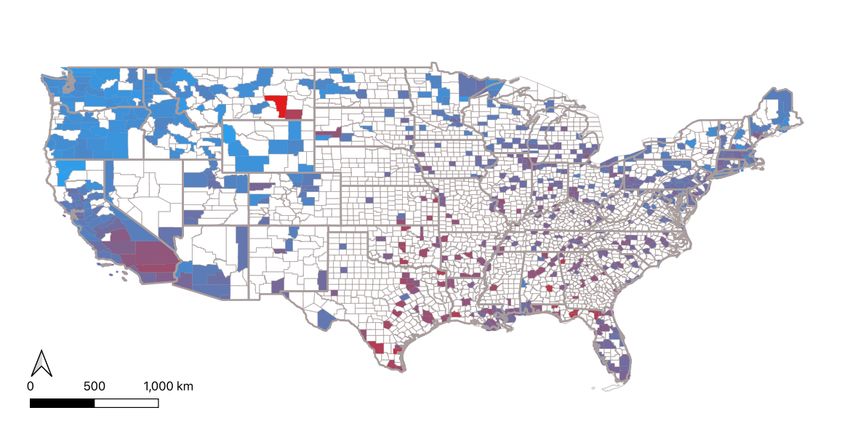
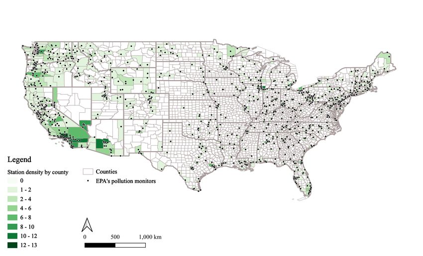
Deryugina et al., 2019). We source fine particulate information from the EPA’s daily outdoor air quality
information, AirNow.3 Monitoring stations with available data from January to August 2020, and their
density by county, are represented in Figure 3. We aggregate monitor air quality information to the county-
day level. In counties with more than one monitoring station, air quality data is weighted by the number
of people in census blocks in a 10 kilometer buffer around the station. Following Deryugina et al. (2019),
the EPA’s air quality monitors are classified into 100 clusters based on their location; these clusters are
represented in Figure 4. Summary statistics are presented in the first panel of Table 1. Figure 5 maps the
mean daily concentration in each month across US counties. We also show the trend in fine particulate
matter levels and air quality index over the course of the pandemic in Figure 6. This figure shows that,
contrary to media portrayals, air pollution levels have remained generally constant over the course of the
pandemic. In addition to PM 2.5 concentrations, AirNow reports Air Quality Index (AQI), which we use as
an alternative air quality measurement for robustness analysis.
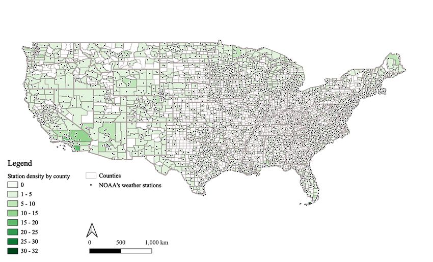
2.3 Wind Speed and Direction
We incorporate information on wind speed and direction from the National Oceanic and Atmospheric Ad-
ministration’s daily weather monitors.4 The data includes weather variables for 2,543 weather stations.5
Figure 7 presents the spatial distribution and density of weather stations. Weather stations have different
reporting frequencies. To address these differences, all reported variables are first aggregated to the station-
hour level and then averaged to the station-day level. Among other weather variables, NOAA’s stations
report information on wind direction and speed.6 Wind direction, measured in degrees, is re-coded as sug-
gested by Deryugina et al. (2019) such that the daily mean wind direction is grouped into four categories
(1o -90o , 91o -180o , 181o -270o , and 271o -360o ). Wind speed is reported in miles-per-hour but is re-coded into
ten dummy variables representing deciles of the speed distribution. We consider three strategies in assigning
NOAA wind direction information to either EPA air quality monitors or to the county. For our main specifi-
cations, each EPA air quality monitor uses a weighted average of the wind direction (in degrees) of the four
nearest weather monitors, which approximates a simple Inverse Distance Weighting (IDW) interpolation as
employed by Deryugina et al. (2019).7 On the other hand, the wind speed data is averaged at the county-day
3 https://www.epa.gov/outdoor-air-quality-data/download-daily-data. Last accessed, September 2, 2020.
4 https://www.ncei.noaa.gov/data/local-climatological-data/archive/2020.tar.gz. Last accessed, September 2, 2020.
5 NOAA reports 2,820 monitoring stations between January and August of 2020. After limiting the stations to the con-
tiguous United States, the number reduces to 2,543.
6 The data also includes information on weather conditions such as precipitation and temperature. Because these variables
are frequently missing, we do not include them as controls in our analysis. P 4
wj DIRjt
7 Therefore, j=1
the assigned wind direction for EPA station i at time t (DIRit ) is given by DIRit = P 4 , where
wj
j=1
DIRjt is the wind direction of the j th nearest weather monitor at time t, and wj = (dij )−1 is the weight of the j th monitor
based on the distance between i and j (dij ).
5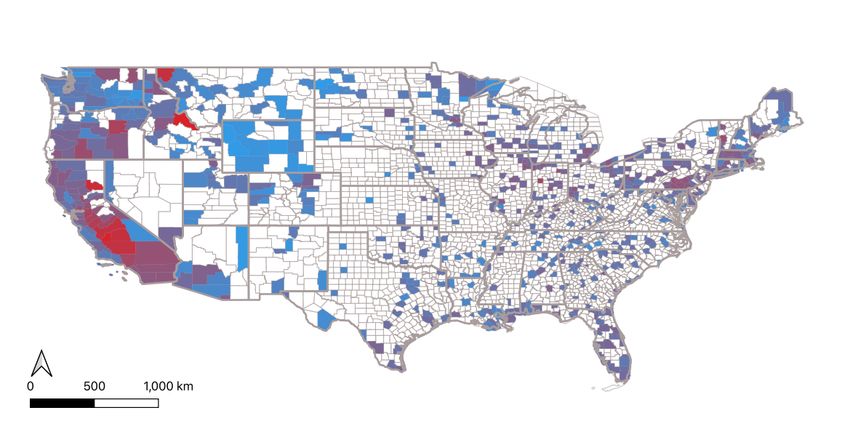
level. We explore the sensitivity of our results to this wind-to-air quality assignment mechanism in Section

5 and more specifically Table A6 and Table A7.

2.4        Social Distancing Metrics

The data company Unacast creates social distancing records by county using cell phone information (Unacast,

2020).8 We use three relevant variables created by Unacast: change to average daily distance traveled from

pre-COVID baseline, change to average daily visits to non-essential locations from pre-COVID baseline, and

change to average daily encounters per square kilometer from baseline. Change to average distance traveled

is a z-score difference in mean distance traveled for all cell phones in a county from the average traveled

distance on the same weekday in a pre-COVID period (March 8th or earlier). The second indicator, change to

average daily visits, controls for essential movements by distinguishing between essential and non-essential

facilities.9 As with change to average distance traveled, changes to visitations are reported as z-scores.

Finally, the rate of encounters captures person-to-person contact. Since Unacast’s underlying cell phone

data do not identify if two people have met, they define person-to-person contact as each time two users are

within 50 meters of each other for 60 minutes or less. This value is then normalized by the counties’ area (in

square kilometers) and compared to a national baseline defined as the average encounters for a pre-outbreak

period (February 10th to March 8th ).10 In all regression specifications, we use the average of all daily values

from the previous 2-week period as control variables. Summary statistics are presented in Table 1.

2.5        State-Level Policy Adoption

We use the COVID-19 Government Response Event Dataset (CoronaNet v1.0) via Safegraph to control for

adoption of aversive policy behavior by state governments (Cheng et al., 2020).11 The full list of policies in-

cludes limiting mass gatherings, social distancing actions, stay at home or quarantine orders, school closures,

testing initiatives, state border closures, public surface cleaning, curfews, information campaigns, state of

emergency declarations, administrative task forces, policies to provide greater access to personal protective

equipment, and other policies to increase access to healthcare resources (such as respirators). For each

county, we create indicator variables equal to one if the policy has started and has not yet ended. Summary

statistics are presented in Table 1.
   8 See  https://www.unacast.com/. Last accessed, September 2, 2020.
   9 Unacast   categorized “essential” based on states’ guidelines. Essential locations include facilities like food stores, pet
stores, and pharmacies, while non-essential facilities include restaurants, department and clothing stores, spas and hair sa-
lons between others. See https://www.unacast.com/post/unacast-updates-social-distancing-scoreboard for more detail on
Unacast’s methodology. Last accessed, September 2, 2020
   10 For more detail on the indicator’s origin and the methodology followed by Unacast, see

https://www.unacast.com/post/rounding-out-the-social-distancing-scoreboard. Last accessed, September 2, 2020
   11 https://www.coronanet-project.org/download.html. Last accessed, September 2, 2020.

                                                                 6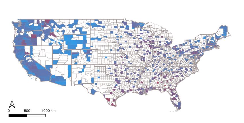
3       Methods

We follow Deryugina et al. (2019) in instrumenting for air pollution with local wind direction, with the

aim of identifying the effect of acute exposure to air pollution on our outcomes of interest. Let P M 2.5iswt

represent the average PM 2.5 concentration in county i, state s, week of the outbreak w, and day t. yiswt

is the health outcome of interest; these outcomes include the daily rate of confirmed COVID-19 cases per

100,000 population, the raw daily count of COVID-19 cases, the rate of confirmed COVID-19 deaths per

100,000 population, and the raw daily count of COVID-19 deaths. We also explore the same case and death

outcomes over 3-day, 7-day, 10-day, and 14-day periods. Consider the following two stage least squares

regression equation:

                                      XX
                     P M 2.5iswt =              βbg 1[Gi = g] ∗ DIRit
                                                                   90b
                                                                       + X 0 γ + ηi + ηsw + νiswt                               (1)
                                      g∈G b=0

                                   yiswt = φP M 2.5iswt + X 0 γ + ηi + ηsw + iswt

     In Equation 1, DIRit represents four wind direction dummies indicating whether average wind direction

falls into one of four 90o quadrants for county i on day t.12 As in Deryugina et al. (2019), variable 1[Gi = g]

is an indicator function asserting that county i belongs to wind monitor group g in the set of all wind

monitor clusters G. Our excluded instruments are the full interaction of wind monitor clusters with wind

direction dummies, or 382 interaction terms. Intuitively, the β coefficients capture how a wind direction

and locality combination influences average PM 2.5 levels in a county on the same day.13 Aside from the

excluded instruments, Equation 1 includes the term X for a suite of time-varying controls for state-level

COVID-19 mitigation policies, day of the week, nine county-level dummies for wind speed categories, two

lagged wind direction-by-cluster variables, and prior 2-week averages of Unacast social distancing metrics

based on cell phone data. Unacast social distancing variables are the change in average distance traveled

from county-level baseline, change in visits from baseline, and change in the rate of human encounters per

square kilometer. We incorporate lagged 2-week averages for these variables to control for behavior over the

relevant incubatory period of COVID-19.14 istw is a random error term clustered at the county level. The
    12 Weomit the wind direction dummy representing 271o -360o .
    13 For
         example, a wind direction is allowed to influence air pollution in the Chesapeake Bay region differently than the
same wind direction in the San Francisco bay region.
   14 We note that social distancing behavior over the previous two-week period may potentially be correlated with air qual-

ity. We take this theoretical possibility seriously and test the sensitivity of our results to alternative specifications in which
we alter the control variables in our model, as shown in Table A2 and Table A3. We further discuss this potential issue in
Section 5.

                                                                 7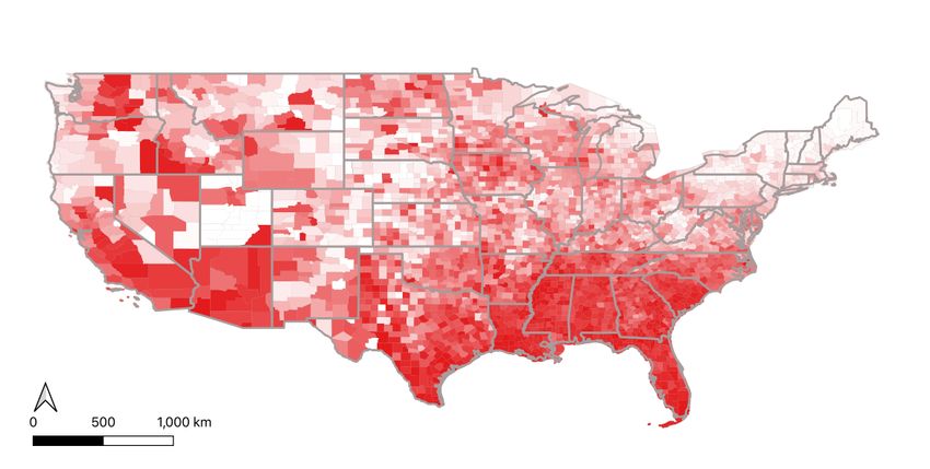
coefficient of interest in Equation 1 is φ, an estimate of the relationship between an additional µg/m3 of PM

2.5 and cases or deaths from COVID-19.

     Equation 1 incorporates county and state-by-week fixed effects, ηi and ηsw .15 These fixed effects control

for time-constant county-level heterogeneity and time-varying state-level characteristics.16 Due to the nature

of the spread of a contagion, the state-by-week fixed effects are best suited for controlling for the evolving

baseline infection rate in a local population, endogenous responses to the infection rate, and the ways in

which underlying heterogeneity may interact with these dynamics. Intuitively, these fixed effects allow

us to ask how better or worse air quality impacts the severity of the COVID-19 outbreak while taking a

ceteris paribus approach with respect to local characteristics, infection rate, and behaviors. For the purpose

of comparison, we also show results with county and metropolitan statistical area-by-week or combined

statistical area-by-week fixed effects specifications.17

     In line with Deryugina et al. (2019), the identifying assumption is that, after flexibly controlling for

the above-mentioned variables, county-level variation in daily wind direction is unrelated to variation in

morbidity and mortality in the same county, if not through variation in air pollution. Hence, this empirical

approach provides quasi-experimental evidence of the effect of air pollution, instrumented by changes in

wind direction, on health outcomes, while addressing common issues identified in the literature, including

measurement error from various sources.

4       Results

4.1         COVID-19 Cases

Contemporaneous exposure to air pollution may influence the severity of illness, thereby increasing the

number of severe cases. Table 2 shows our primary results on confirmed cases across a range of fixed effects

specifications. In columns (1) through (3), we show the relationship between PM 2.5 and case rates per

100,000 individuals in a county. Columns (4) through (6) regress wind-fitted PM 2.5 on case totals. In

column (1), we find that an increase of one µg/m3 of fine particulate matter in a county will increase the
    15 To this end, we use the Stata command ivreghdf e (Correia, 2016).
    16 The use of state-by-week fixed effects, or within-week comparisons, imply that we are not investigating how air quality
affects the speed of transmission of the virus but rather how air quality affects the severity of illness among already-infected
individuals. Confirmed cases are expected to represent more severe cases, for which infected individuals experience symp-
toms and seek testing (Day, 2020; Gandhi et al., 2020). We do not expect air pollution to change the threshold of pain and
symptoms leading individuals to seek testing, but rather to increase the number of people whose pain and symptoms exceed
such threshold. We also note that identifying the speed of transmission is beyond the scope of our paper. The often-lengthy
incubation period, testing lags, and reporting lags mean that our estimation procedure does not identify the speed of trans-
mission.
   17 In each of these specifications, counties that are not in an MSA or CBSA are assigned state-by-week fixed effects. For

example, a county and MSA-by-week fixed effects specification would make within-MSA, within-week comparisons for MSAs,
while rural regions would be compared to other non-MSA regions in the same state and week. To avoid over-fitting, any
MSA or CBSA with only one county is also assigned the state-by-week fixed effect.

                                                               8
number of confirmed cases per 100,000 population by 0.13. This is roughly a 2% increase from the mean case
rate per county on a given day. In columns (2) and (3), we show that this increase is roughly constant at
0.12 and 0.11 when adopting MSA-by-week or CBSA-by-week fixed effects. In our regressions on total cases
in columns (4) through (6), a one unit increase of PM 2.5 in a county results in 4-5 additional cases within a
county on the same day. These estimates reflect larger percent changes from the mean than those observed
on case rates, and they are consistent across fixed effects specifications. However, our point estimates are
less-precisely estimated in regressions on case totals.
We quantify the magnitude of these findings in two ways. First, the within-county standard deviation of
average daily PM 2.5 over our sample period is 3.6 µg/m3 . Therefore, a wind-induced shift in PM 2.5 of one
standard deviation would be expected to increase cases in any given county by at least 6% from the mean.
Second, we estimate the approximate change over the support of wind-induced PM 2.5 shifts. We incorporate
four wind-direction dummies. Within any county, the wind direction associated with lowest PM 2.5 levels
has an average PM 2.5 level of 4.9 µg/m3 ; the second is 5.9, third is 6.9, and the highest wind direction is
associated with mean PM 2.5 level of 7.9 µg/m3 . These categories illustrate that any given county has wide
variation in PM 2.5 levels associated with wind direction, ranging an average of 3 µg/m3 from lowest to
highest wind direction-pollution combination. Therefore, any given county would be expected to see at least
5% more confirmed cases on the worst wind-pollution combination days in comparison to the best ones, or
at least a 1.7% increase in confirmed cases from even a slight step up in PM 2.5 associated with a marginal
change in wind direction. For comparison, Persico and Johnson (2020) found that a one unit increase in fine
particulate matter led to an approximate doubling of confirmed cases and deaths. Recall that the effects
in Persico and Johnson (2020) are induced by regulatory rollback of pollution control at Toxic Release
Inventory sites. Because these sites release many harmful pollutants other than fine particulate matter, it
seems reasonable that the magnitude of their findings would be higher than those we observe. Further,
populations especially exposed to pollution from Toxic Release Inventory sites may be more vulnerable for
a variety of reasons, including past exposure to the many harmful pollutants released at those sites. Persico
and Johnson (2020) analyze heterogeneous effects along standard socioeconomic dimensions and find worse
pollution exposure for counties with a higher fraction of Black individuals, with higher unemployment, and
with lower incomes. Our approach allows isolating the effect of PM 2.5 while inferring from a much broader
set of pollution sources, thus generalizing previous results. A wide set of policy implications follow from our
empirical findings, which we discuss in Section 6.
Further, we show how air pollution impacts the number of cases over the following 3, 7, 10, and 14 day
periods in Table 4. For concision, we show only specifications with county and state-by-week fixed effects.18
18 All additional estimations are available by the authors upon request.
9In column (1), we see our previous result that a one µg/m3 increase in PM 2.5 increases the case rate by
0.13 and the total cases by 5.4 on the same day. Column (2) of the table suggests that a one unit increase in
fine particulate matter in a given county is expected to increase the number of cases per 100,000 by 0.3 over
the following three day period. While this effect in magnitude is over twice as large, it is a smaller percent
increase relative to the mean 3-day combined case rate at 1.5%. Meanwhile, the same one unit increase
would be expected to increase the case rate by 0.17 over a seven day period, 0.37 over a ten-day period
and by 0.43 over a two week period. It seems reasonable that the magnitude of the findings would increase
over longer time horizons, as a given exposure to pollution may lead the severity of cases to increase over
several days, and testing or reporting lags may further delay the time of confirmation. At the same time,
our estimates tend to become noisier over longer time horizons. In the second panel of Table 4, we observe
a similar increasing relationship between PM 2.5 and confirmed cases when our outcome is total cases. The
relationship between a one unit increase in PM 2.5 and confirmed cases over three days is 23, four times
higher than the magnitude of our same-day estimations. Over two weeks, the relationship increases to 111
additional confirmed cases per unit of PM 2.5, or a 22% increase from the mean 2-week case total.
4.2 COVID-19 Deaths
Table 3 displays point estimates for the relationship between levels of fine particulate matter and confirmed
COVID-19 deaths. As in Table 2, columns (1) through (3) display results on death rates per 100,000
individuals, while columns (4) through (6) show the relationship between PM 2.5 and death totals. The
point estimate in column (1) suggests that an additional unit of wind-induced PM 2.5 would raise the same-
day death rate from COVID-19 by 0.006. This is a 3% increase from the mean daily death rate within
a county of 0.18. This coefficient is generally stable when adopting MSA-by-week or CBSA-by-week fixed
effects in place of the state-by-week fixed effects, as displayed in column (2) and column (3). Meanwhile, our
estimates in columns (4) through (6) suggest that a one-unit increase in PM 2.5 would increase the absolute
death count by 0.07 - 0.09, or roughly a 7% increase from the mean number of COVID-19 deaths in a county
on any given day. For comparison, the cross-sectional estimates in Wu et al. (2020) suggest, if taken at face
value, that a µg/m3 increase in average historical exposure to PM 2.5 is associated with an 8% increase in
the rate of deaths from COVID-19.
Finally, consistent with Deryugina et al. (2019), we examine the relationship between exposure to an
additional unit of PM 2.5 and COVID-19 deaths over longer time horizons. The corresponding estimates are
provided in Table 5. For death rates, we show that the relationship remains roughly constant at 0.006 for up
to three days, but then we observe no discernible relationship between exposure to PM 2.5 and death rates
10over 7, 10, and 14 day periods. Conversely, we observe a slightly increasing relationship between exposure
to PM 2.5 and death totals over up to two week periods, with a single unit of PM 2.5 exposure increasing
two-week death counts by approximately 2 individuals per county, an 11% increase from the mean two-week
county death rate of 17. Our results suggest that a county would have 33% fewer deaths if wind came
from the least-polluted direction for two weeks, in comparison to itself if wind came from the most-polluted
direction for two weeks.
5 Robustness Tests
In this section, we assess the sensitivity of our results to a battery of alternative specifications. We proceed
as follows. First, we re-examine our relationship of interest when replacing PM 2.5 with EPA’s Air Quality
Index as independent variable. Second, we test the sensitivity of our results to inclusion of different time-
varying daily controls. In particular, we show how our results compare when dropping social distancing
metrics. Third, we drop New York City, which may be considered a special case in the context of the
COVID-19 epidemic. Fourth, we compare our instrumental variable approach to estimations using Ordinary
Least Squares. Fifth, we explore alternate mechanisms for assigning wind and weather information to air
quality monitors.
AQI vs. PM 2.5: We use PM 2.5 as our primary independent variable to represent air pollution, although
a variety of air pollutants contribute to air quality. We therefore also test our primary regression specification
with EPA’s Air Quality Index (AQI) as the independent variable. As with PM 2.5, we construct this variable
by population-density weighting AQI measures when more than one monitor is present in a county. The
results are presented in Table A1. In all regression specifications, the relationship between AQI and COVID-
19 morbidity and mortality is of the same sign and similar statistical significance as the relationship between
PM 2.5 and COVID-19 morbidity and mortality. For case rates, the relationship is actually much more
precisely estimated across all fixed effects specifications, although death rate point estimates have slightly
less statistical significance. The magnitude of the point estimates, however, are consistent across PM 2.5
and AQI if not slightly larger for AQI. For example, we see that a one unit increase in AQI in a county
would lead to a 0.6% increase in case and a 0.8% increase in death rates. Scaling these by the mean AQI,
which is four times as large as the mean PM 2.5, results in similar shifts from PM 2.5 in the range of 2%
and 3%, respectively. The fact that the magnitude is of similar range, if not slightly larger, makes sense, as
fine particulate matter is not the only harmful air pollutant that may exacerbate COVID-19 outcomes.
11Inclusion of Different Time-Varying Controls: Our primary regressions control for state-level policies
to control the spread of COVID-19, wind speed dummies, past 2-week average social distancing information,
day of the week, and two days of lagged wind-direction combinations. In Table A2, we show how our primary
results differ when subsets of controls are used. In columns (1) and (5), we show how our results differ when
no controls are adopted except lagged wind-direction combination. Coefficients for case rates and counts, as
well as death rates and counts, are all less-precisely estimated. Point estimates for case or death rates are
half as large as our primary estimates, although estimates for case or death totals are similar, even slightly
larger, than our primary estimates. When adding day of week and wind speed dummies, our results for case
and death rates are larger and more precisely-estimated, achieving statistical significance for case rates and
near significance for death rates. Incorporating either state-level policies or social distancing controls, in
columns (3), (4), (7), and (8), very slightly improves the precision of our estimates in most specifications.
However, the magnitude of the point estimates remains roughly constant across all specifications. If anything,
this evidence compounds that provided in Deryugina et al. (2019) on the validity of wind direction as an
instrument for air pollution.
With respect to case rates and death rates, inclusion of past 2-week average social distancing controls
slightly elevates our point estimates, while case counts and death counts appear unaffected. In Table A3,
we test how our primary results differ when excluding all past 2-week average social distancing metrics.
Point estimates are similar in all models, although we note that slight attenuation does occur in most
specifications. Hence, we conclude that our approach is able to capture the main effect of interest, even
if past 2-week average social distancing behavior may be correlated with pollution through two channels,
avoidance behavior (Graff Zivin and Neidell, 2009; Neidell, 2009; Deschênes et al., 2017) and the fact that
past social distancing behavior may generate less pollution.
Drop New York City: The first major outbreak of COVID-19 in the continental United States occurred
in the metropolitan region surrounding New York City, a large and heavily-populated zone with unique
characteristics with respect to its outbreak intensity, COVID-19 response, and pollution levels. In Table A4,
we test whether our results differ when excluding this region from the sample.19 In virtually all specifications,
our results are larger in magnitude and more precisely estimated when excluding New York City. With the
exception of death counts, we observe highly statistically significant relationships between an additional
unit of PM 2.5 and each outcome. For example, in column (1), we observe that an additional unit of PM
2.5 increases case rates per 100,000 individuals by 0.15, a 2.4% increase. In comparison, our estimations
including New York City showed an increase of 0.13 cases, or a 2% increase. The increase in case counts is
19 We exclude the counties or boroughs of Nassau, Westchester, Queens, Manhattan, Brooklyn, and the Bronx. Corre-
sponding FIPS codes for these regions are 36059, 36119, 36081, 36061, 36047, and 36005.
12now 6-7 additional confirmed COVID-19 cases per unit of PM 2.5. Though still statistically insignificant,
these point estimates are more precisely estimated than our results including New York City. Meanwhile,
the increase in the death rate, now highly significant, is 0.009 instead of 0.006 per 100,000 individuals, a 5%
increase instead of a 3% increase. Regressions on total deaths, previously a statistically insignificant 0.08 or
7% per additional unit of PM 2.5, are now a sizeable and statistically significant 0.3, a 34% from the mean
daily death count. From these results, we conclude that our findings are robust to the exclusion of the New
York City region.
Instrumental Variables vs. Ordinary Least Squares: The previous literature has identified mea-
surement error as one of the main issues when analyzing the effect of air pollution on health outcomes,
thus leading to the use of an instrumental variable approach to overcome it (Deryugina et al., 2019). This
approach can also tackle other non-random sources of variation in the pollution-health relationship, which
also limit the extent to which naive estimations via Ordinary Least Squares may lead to causal estimates.
As per standard procedure, we compare estimates obtained with the instrumental variable approach to es-
timates obtained via Ordinary Least Squares to ascertain the direction and magnitude of the bias, if any.
In Table A5, we show the reduced-form relationship between concentrations of fine particulate matter and
confirmed cases and deaths on the same day, using Ordinary Least Squares. We estimate these relationships
across the same fixed effects as before. In the first panel and first column of Table A5, we see that an
additional unit of PM 2.5 is associated with a 0.03 increase in the case rate per 100,000 population. This is
a 0.4% increase relative to the mean daily case rate in a county. Similarly, in column (4) we see that a one
unit increase in PM 2.5 is associated with 6 additional confirmed cases in a county. While these coefficients
are of the same sign as our baseline point estimates, they are less precisely estimated. In the case of case
rates, they are also much smaller in magnitude, reflecting a 0.4% change from an additional unit of PM 2.5
instead of a 2% shift. Ordinary Least Squares coefficients are essentially zero for all regressions on death
rates; for death counts, the coefficients are of the same sign as our instrumental variable point estimates but
one tenth the magnitude. The standard errors are also approximately four times as large as the coefficient.
For comparison, our instrumental variable estimates suggest an additional unit of PM 2.5 raises the daily
death count by 0.08, while the Ordinary Least Squares estimate is 0.008. Hence, our comparison of estimates
between our main specifications and Ordinary Least Squares tends to confirm the conclusion of Deryugina
et al. (2019) on the influence of measurement error in naive regressions.
Matching Weather Stations to Air Quality Monitors: We assign wind direction variables to air
quality monitors by inverse-distance weighting wind direction values of the four nearest weather stations.
13This assignment mechanism approximates that of Deryugina et al. (2019), in which a complete national
wind direction and speed interpolation allows flexible assignment of wind variables to any given air qual-
ity monitor location.20 We also present results under two alternative assignment mechanisms. First, we
assign wind direction based on only the closest weather station.21 Next, we assign wind direction based
on inverse-distance weighting wind direction values of the twelve nearest weather stations. We present our
main empirical specifications with these alternate wind direction assignments in Table A6 and Table A7.
When assigning wind direction based on only the closest weather station, our results on cases are virtually
unchanged. However, we note slight attenuation in our point estimates on death rates as well as imprecise
estimates on death totals. Meanwhile, when assigning wind direction based on the twelve nearest weather
stations, all coefficients are very similar to our baseline estimations, with all coefficients in regressions on
death rates or counts are of larger magnitude. These results suggest that use of a single weather station to
assign wind direction may noisily capture weather patterns in the surrounding region, while our estimates
are robust to averaging wind direction over up to twelve nearest weather stations.
6 Policy Relevance
Our findings indicate that higher contemporaneous exposure to PM 2.5 leads to higher COVID-19 morbidity
and mortality. While concentrations of PM 2.5 may have decreased in some cities across the United States
in the early days of the COVID-19 outbreak (see Berman and Ebisu, 2020), we observe little change in PM
2.5 or AQI levels nationwide over the course of the pandemic. Further, Persico and Johnson (2020) report
an increase in particulate matter in counties with TRI sites since the pandemic began, suggesting that
environmental deregulation may have largely offset any decrease in air pollution driven by less motorized
traffic. Figure 6 shows a pattern consistent with these elements. Meanwhile, the overall number of COVID-
19 cases and deaths has continued to increase in the United States as well as globally. It follows from our
findings that there is a continued rationale for limiting pollution levels while reopening the economy. In
this section, we discuss several policy levers that may be used by policymakers at the federal, state, and
local level. Private companies may also contribute to keep current pollution down as part of their corporate
social responsibility strategies by letting employees telework whenever appropriate. As suggested in Persico
and Johnson (2020), hospitals may consider using air purifiers in rooms with COVID-19 patients, to limit
exposure to air pollution and prevent the need for ventilators.
At the federal level, reinstating air pollution control and reporting regulations, requirements lifted in
20 Deryugina et al. (2019) use the North American Regional Reanalysis (NARR) daily reanalysis data. Since our study
uses contemporaneous wind and air quality information, NARR data is not yet readily available for our sample time period.
21 If the nearest weather station is missing wind information for a given day, we assign wind variables based on the second-
closest weather station.
14March 2020, may lower releases by large polluting sites and thereby improve COVID-19 morbidity and
mortality outcomes. Additional immediate policy levers may emerge in case of a new recovery package,
which could complement the Coronavirus Aid, Relief, and Economic Security (CARES) Act of March 27th
2020. Relief funds could, for instance, be provided to some industries conditional on pollution reductions.
Airlines are a case in point. The CARES Act required airline companies to maintain a minimum number of
flights between destinations that were served before the outbreak started. Many of those flights are likely
to be carried out at very low levels of capacity, thus generating pollution at the same time that they create
operational losses to the airlines. Renegotiating the terms of the agreement in the light of our findings may
be in the interest of both society and the airlines.
State regulations can limit the extent with which people can move for non-essential activities and encour-
age continued teleworking as much as possible, in case voluntary efforts by companies are deemed insufficient.
Local governments can also regulate traffic and pollution directly. For instance, adjusting speed limits on
highways to current traffic conditions can reduce pollution (Bel and Rosell, 2013). Temporary policies using
alternate license plates can be enforced for non-essential movements, for instance allowing individuals with
an even final digit on the license plate number to circulate only on even days of the month (Davis, 2008;
Gallego et al., 2013; Li, 2018). Retrofitted public transit vehicles can be used whenever possible (Beatty and
Shimshack, 2011; Austin et al., 2019), especially as long as the number of routes and the frequency of service
have both been adjusted downward during the outbreak. To the extent that it is feasible in the short run,
expanding current public transit infrastructure would also contribute to limit local air pollution (Lalive et al.,
2018; Li et al., 2019). Expanding subsidies for electric and hybrid vehicles as well as charging stations may
also accelerate the transition to cleaner vehicles (Beresteanu and Li, 2011; Li et al., 2017; Muehlegger and
Rapson, 2018), depending on the local context (Holland et al., 2016), the expected duration of the current
pandemic (Scudellari, 2020), as well as expectations about future ones.
Many of these policy implications apply also to other countries in the world. Further, all cities with
congestion charges already in place, such as Gothenburg, London, Milan, Singapore, or Stockholm, may
consider adjusting the price level to reflect current pollution levels and the spread of COVID-19 (Coria
et al., 2015). Congestion charges have indeed been shown to reduce overall traffic and pollution (Leape,
2006; Gibson and Carnovale, 2015). Several cities around the world also limit access to city centers or entire
regions to some vehicles, depending on vintage, fuel type, and efficiency (e.g., Barahona et al., 2019). Such
regulations may also be adjusted during the pandemic. Over the longer run, COVID-19-related deaths could
be used as an additional impetus to internalize known externalities from local air pollution (e.g. Parry and
Small, 2005; Muller and Mendelsohn, 2009).
157 Conclusion
The novel Coronavirus has caused hundreds of thousands of deaths and severe economic damage across the
world. The common experience of many countries has shown that a trade-off exists between the speed at
which economic activity is relaunched and the risk of further cases and deaths. This trade-off is usually
described as between two important but conflicting goals: jobs and economic recovery on one side, and
limiting cases and deaths on the other. Our paper adds one dimension to this trade-off, pointing to an
untapped potential to limit severe cases and deaths while sustaining economic recovery. Our study shows
that the observed trade-off between the two aforementioned desirable goals can be relaxed by keeping current
pollution at low levels. Indeed, we find strong evidence that current air quality almost immediately affects
the severity of COVID-19 illness. According to our results, a one µg/m3 increase in PM 2.5 (about 15%
of the average concentration of PM 2.5) increases the number of severe cases by roughly 2% and same-day
deaths by 3% from the mean case rate in a county. Our results rely on arguably exogenous variation in
wind direction and are robust to a wide variety of specifications. Overall, our study points to a potentially
important role for policy levers aimed at lowering pollution in addressing the pandemic.
16References
Ackermann, M., S. E. Verleden, M. Kuehnel, A. Haverich, T. Welte, F. Laenger, A. Vanstapel, C. Werlein,
H. Stark, A. Tzankov, W. W. Li, V. W. Li, S. J. Mentzer, and D. Jonigk (2020). Pulmonary vascular
endothelialitis, thrombosis, and angiogenesis in Covid-19. New England Journal of Medicine 383 (2),
120–128.
Anderson, M. L. (2020). As the wind blows: The effects of long-term exposure to air pollution on mortality.
Journal of the European Economic Association 18 (4), 1886–1927.
Arceo, E., R. Hanna, and P. Oliva (2016). Does the effect of pollution on infant mortality differ between
developing and developed countries? Evidence from Mexico City. The Economic Journal 126 (591), 257–
280.
Austin, W., G. Heutel, and D. Kreisman (2019). School bus emissions, student health and academic perfor-
mance. Economics of Education Review 70, 109–126.
Barahona, N., F. A. Gallego, and J.-P. Montero (2019). Vintage-specific driving restrictions. The Review of
Economic Studies 87 (4), 1646–1682.
Beatty, T. K. M. and J. P. Shimshack (2011). School buses, diesel emissions, and respiratory health. Journal
of Health Economics 30 (5), 987–999.
Bel, G. and J. Rosell (2013). Effects of the 80km/h and variable speed limits on air pollution in the
metropolitan area of Barcelona. Transportation Research Part D: Transport and Environment 23, 90–97.
Beresteanu, A. and S. Li (2011). Gasoline prices, government support, and the demand for hybrid vehicles
in the United States. International Economic Review 52 (1), 161–182.
Berman, J. D. and K. Ebisu (2020). Changes in u.s. air pollution during the covid-19 pandemic. Science of
The Total Environment 739, 139864.
Bishop, K. C., J. D. Ketcham, and N. V. Kuminoff (2018). Hazed and confused: The effect of air pollution
on dementia. Report 0898-2937, National Bureau of Economic Research.
Brodeur, A., D. M. Gray, A. Islam, and S. Bhuiyan (2020). A literature review of the economics of Covid-19.
SSRN Scholarly Paper ID 3636640, Social Science Research Network, Rochester, NY.
Chay, K., C. Dobkin, and M. Greenstone (2003). The Clean Air Act of 1970 and adult mortality. Journal
of Risk and Uncertainty 27 (3), 279–300.
Chay, K. and M. Greenstone (2003). The impact of air pollution on infant mortality: Evidence from geo-
graphic variation in pollution shocks induced by a recession. The Quarterly Journal of Economics 118 (3),
1121–1167.
Chen, Y., A. Ebenstein, M. Greenstone, and H. Li (2013). Evidence on the impact of sustained exposure to
air pollution on life expectancy from China’s Huai River policy. Proceedings of the National Academy of
Sciences of the United States of America 110 (32), 12936–12941.
Cheng, C., J. Barceló, A. Hartnett, R. Kubinec, and L. Messerschmidt (2020). Covid-19 government response
event dataset (coronanet v1.0).
Coria, J., J. Bonilla, M. Grundström, and H. Pleijel (2015). Air pollution dynamics and the need for
temporally differentiated road pricing. Transportation Research Part A: Policy and Practice 75, 178–195.
Correia, S. (2016). Linear models with high-dimensional fixed effects: An efficient and feasible estimator.
Working Paper.
Currie, J. and M. Neidell (2005). Air pollution and infant health: What can we learn from California’s recent
experience? The Quarterly Journal of Economics 120 (3), 1003–1030.
17Currie, J. and R. Walker (2011). Traffic congestion and infant health: Evidence from E-ZPass. American
Economic Journal: Applied Economics 3 (1), 65–90.
Currie, J., J. G. Zivin, J. Mullins, and M. Neidell (2014). What do we know about short- and long-term
effects of early-life exposure to pollution? Annual Review of Resource Economics 6 (1), 217–247.
Davis, L. W. (2008). The effect of driving restrictions on air quality in Mexico City. Journal of Political
Economy 116 (1), 38–81.
Day, M. (2020). Covid-19: Four fifths of cases are asymptomatic, China figures indicate. BMJ 369.
Deryugina, T., G. Heutel, N. H. Miller, D. Molitor, and J. Reif (2019). The mortality and medical costs of
air pollution: Evidence from changes in wind direction. American Economic Review 109 (12), 4178–4219.
Deschênes, O., M. Greenstone, and J. S. Shapiro (2017). Defensive investments and the demand for air
quality: Evidence from the NOx Budget Program. American Economic Review 107 (10), 2958–2989.
Ebenstein, A., L. Victor, and R. Sefi (2016). The long-run economic consequences of high-stakes exam-
inations: Evidence from transitory variation in pollution. American Economic Journal: Applied Eco-
nomics 8 (4).
EPA (2019). Integrated science assessment (ISA) for particulate matter. Technical Report EPA/600/R-
19/188, U.S. Environmental Protection Agency, Washington, DC.
Gallego, F., J.-P. Montero, and C. Salas (2013). The effect of transport policies on car use: Evidence from
Latin American cities. Journal of Public Economics 107, 47–62.
Gandhi, M., D. S. Yokoe, and D. V. Havlir (2020). Asymptomatic transmission, the Achilles’ heel of current
strategies to control Covid-19. New England Journal of Medicine 382 (22), 2158–2160.
Gibson, M. and M. Carnovale (2015). The effects of road pricing on driver behavior and air pollution. Journal
of Urban Economics 89, 62–73.
Graff Zivin, J. and M. Neidell (2009). Days of haze: Environmental information disclosure and intertemporal
avoidance behavior. Journal of Environmental Economics and Management 58 (2), 119–128.
He, J., H. Liu, and A. Salvo (2019). Severe air pollution and labor productivity: Evidence from industrial
towns in China. American Economic Journal: Applied Economics 11 (1), 173–201.
Holland, S. P., E. T. Mansur, N. Z. Muller, and A. J. Yates (2016). Are there environmental benefits from
driving electric vehicles? The importance of local factors. American Economic Review 106 (12), 3700–3729.
Knittel, C. R., D. L. Miller, and N. J. Sanders (2016). Caution, drivers! children present: Traffic, pollution,
and infant health. The Review of Economics and Statistics 98 (2), 350–366.
Lalive, R., S. Luechinger, and A. Schmutzler (2018). Does expanding regional train service reduce air
pollution? Journal of Environmental Economics and Management 92, 744–764.
Lavy, V., A. Ebenstein, and S. Roth (2012). The impact of air pollution on cognitive performance and
human capital formation.
Leape, J. (2006). The London Congestion Charge. Journal of Economic Perspectives 20 (4), 157–176.
Li, S. (2018). Better lucky than rich? Welfare analysis of automobile licence allocations in Beijing and
Shanghai. The Review of Economic Studies 85 (4), 2389–2428.
Li, S., Y. Liu, A.-O. Purevjav, and L. Yang (2019). Does subway expansion improve air quality? Journal of
Environmental Economics and Management 96, 213–235.
Li, S., L. Tong, J. Xing, and Y. Zhou (2017). The market for electric vehicles: Indirect network effects and
policy design. Journal of the Association of Environmental and Resource Economists 4 (1), 89–133.
18Luechinger, S. (2014). Air pollution and infant mortality: A natural experiment from power plant desulfur-
ization. Journal of Health Economics 37, 219–231.
Muehlegger, E. and D. S. Rapson (2018). Subsidizing mass adoption of electric vehicles: Quasi-experimental
evidence from California. Working Paper 25359, National Bureau of Economic Research.
Muller, N. Z. and R. Mendelsohn (2007). Measuring the damages of air pollution in the United States.
Journal of Environmental Economics and Management 54 (1), 1–14.
Muller, N. Z. and R. Mendelsohn (2009). Efficient pollution regulation: Getting the prices right. American
Economic Review 99 (5), 1714–1739.
Neidell, M. (2009). Information, avoidance behavior, and health: The effect of ozone on asthma hospitaliza-
tions. Journal of Human Resources 44 (2), 450–478.
Parry, I. W. H. and K. A. Small (2005). Does Britain or the United States have the right gasoline tax?
American Economic Review 95 (4), 1276–1289.
Persico, C. and K. R. Johnson (2020). Deregulation in a time of pandemic: Does pollution increase coron-
avirus cases or deaths? (13231).
Sanders, N. J. (2012). What doesn’t kill you makes you weaker: Prenatal pollution exposure and educational
outcomes. Journal of Human Resources 47 (3), 826–850.
Scudellari, M. (2020). How the pandemic might play out in 2021 and beyond. Nature 584 (7819), 22–25.
Simeonova, E., J. Currie, P. Nilsson, and R. Walker (2018). Congestion pricing, air pollution and children’s
health. Working Paper 24410, National Bureau of Economic Research. Series: Working Paper Series.
Unacast (2020). Unacast social distancing dataset. https://www.unacast.com/data-for-good. Version from
17 April 2020.
Wu, X., R. C. Nethery, B. M. Sabath, D. Braun, and F. Dominici (2020). Exposure to air pollution and
COVID-19 mortality in the United States: A nationwide cross-sectional study. medRxiv .
19You can also read


