Curvilinear mesh adaptation
←
→
Page content transcription
If your browser does not render page correctly, please read the page content below
Curvilinear mesh adaptation

Ruili Zhang, Amaury Johnen and Jean-François Remacle

Abstract This paper aims at addressing the following issue. Assume a unit
square: Ω = {(x1 , x2 ) ∈ [0, 1] × [0, 1]} and a Riemannian metric gij (x1 , x2 )
defined on U . Assume a mesh T of U that consist in non overlapping valid
quadratic triangles that are potentially curved. Is it possible to build a unit
quadratic mesh of U i.e. a mesh that has quasi-unit curvilinear edges and
quasi-unit curvilinear triangles ? This paper aims at providing an embryo of
solution to the problem of curvilinear mesh adaptation. The method that is
proposed is based on standard differential geometry concepts. At first, the
concept of geodesics in Riemannian spaces is quickly presented: the geodesic
between two points as well as the unit geodesic starting at a given point
with a given direction are the two main tools that allow us to address our
issue. Our mesh generation procedure is done in two steps. At first, points are
distributed in the unit square U in a frontal fashion, ensuring that two points
are never too close to each other in the geodesic sense. Then, a simple isotropic
Delaunay triangulation of those points is created. Curvilinear edge swaps as
then performed in order to build the unit mesh. Notions of curvilinear mesh
quality is defined as well that allow to drive the edge swapping procedure.
Examples of curvilinear unit meshes are finally presented.

Ruili Zhang
Université catholique de Louvain, Avenue Georges Lemaitre 4, bte L4.05.02, 1348 Louvain-
la-Neuve, Belgium, e-mail: ruili.zhang
Amaury Johnen
Université catholique de Louvain, Avenue Georges Lemaitre 4, bte L4.05.02, 1348 Louvain-
la-Neuve, Belgium, e-mail: amaury.johnen@uclouvain.be
Jean-François Remacle
Université catholique de Louvain, Avenue Georges Lemaitre 4, bte L4.05.02, 1348 Louvain-
la-Neuve, Belgium, e-mail: jean-francois.remacle@uclouvain.be

                                                                                       1
2                           Ruili Zhang, Amaury Johnen and Jean-François Remacle

1 Introduction

There is a growing consensus that state of the art Finite Volume and Fi-
nite Element technologies require, and will continue to require too extensive
computational resources to provide the necessary resolution, even at the rate
with which computational power increases. The requirement for high resolu-
tion naturally leads us to consider methods with higher order of grid conver-
gence than the classical (formal) 2nd order provided by most industrial grade
codes. This indicates that higher-order discretization methods will replace at
some point the finite volume/element solvers of today, at least for part of
their applications. The development of high-order numerical technologies for
CFD is underway for many years now. For example, Discontinuous Galerkin
methods (DGM) have been largely studied in the literature, initially in a
quite theoretical context [4], and now in the application point of view [9].
In many contributions, it is shown that the accuracy of the method strongly
depends of the accuracy of the geometrical discretization [3] In other words,
the following question is raised: yes we have the high order methods, but how
do we get the meshes?
   Several research teams are now actively working in the domain of curvilin-
ear meshing. This new subject is considered as crucial for the future of CFD
[13] and large fundings have been given to some brilliant researchers to allow
innovation in the domain (our colleague Xevi Roca has recently obtained an
ERC starting grant on the subject).
   A good research project should ideally be summarized as a simple yet
fundamental question. It is very much the case here. Assume a unit square

                        Ω = {(x1 , x2 ) ∈ [0, 1] × [0, 1]}

and a smooth function f (x1 , x2 ) defined on the square. Consider a mesh T
made of P 2 triangles that exactly covers the square. How can we compute
the mesh T that minimizes the discretization error kΠf − f kΩ . Here, Π is
the so-called Clément interpolation of f on the mesh [5]. This problem is
the problem of curvilinear mesh adaptation . The solution of that problem
requires to address three main open questions:
1. What is the geometrical structure of the discretization error in the P 2
   case?
2. How can we relate this structure with the geometry/shape of a P 2 triangle?
3. How can we build a mesh made of optimal P 2 triangles?
The first question is related to error estimation and we will not deal with it
in this paper.
   In this first attempt, we will start with a simpler statement. A Riemannian
metric field gij (x1 , x2 ) is defined on the unit square. This metric field is
supposed to be the result of the error estimation. Our aim is thus to build
a unit P 2 mesh with respect to that metric. A discrete mesh T of a domain
Curvilinear mesh adaptation 3
Ω is a unit mesh with respect to Riemannian metric space g(x1 , x2 ) if all its
elements are quasi-unit. More specifically, a curvilinear triangle t defined by
its list of edges ei , i = 1, 2, 3 is said to be quasi-unit if all its adimensional
edges lengths Lei ∈ [0.7, 1.4]1 . Generating unit straight-sided meshes is a
problem that has been largely studied, both in the theoretical point of view
and on the application point of view [6]. Here, our aim is to allow edges to
become curved, leading to unit meshes that would potentially contain way
less triangles.
The paper is structured as follows. Our mesh generation technique essen-
tially relies on the computation of the shortest parabola between two points
and on a unit-size parabola starting in a given direction. In Section 2, stan-
dard notions of geodesics in Riemann spaces are briefly exposed. Algorithms
that compute geodesic parabolas are explained as well.
The mesh generation approach that we advocate is in two steps. We first
generate the points in a frontal fashion [1]. In that process, we ensure that
(i) two points xi and xj are never too close to each other and (ii) that there
exist four points xij , j = 1, . . . , 4 in the vicinity of each point xi that are not
too far to xi i.e. that can form edges in the prescribed range [0.7, 1.4].
Then, points are connected in a very standard “isotropic” fashion. The
mesh is subsequently modified using curvilinear edge swaps in order to form
the desired unit mesh. A curvilinear mesh quality criterion is proposed that
allow to drive the edge swapping process.
In §5, some unit meshes are presented that adapt to analytical metric
fields.
In what follows, we illustrate concepts of unit circle and geodesics using
the following toy metric tensor :
1
!
0
1 2 g11 g12 cos θ sin θ 2
lmin cos θ − sin θ
g(x , x ) = = (1)
g12 g22 − sin θ cos θ 0 l21 sin θ cos θ
max
with
x = {x1 , x2 }, r = kxk, θ = arctan(x2 /x1 ),
lmin = + lmax (1 − exp(−((r − r0 )/h)2 ).
2 Geodesics
In a Riemannian space, the length of curve C is computed as
Z q
LC = gij dxi dxj
C
1 This range is not arbitrary. When a long edge of size 1.4 is split, it should not become a
√ √
short edge. Other authors choose [ 2/2, 2]4 Ruili Zhang, Amaury Johnen and Jean-François Remacle
The geodesic between two points x1 and xs is the shortest path C between
those two points. It is possible to compute geodesics by solving a set of cou-
pled ordinary differential equation (ODE). Defining the so-called Christoffel
symbols
i 1 −1 ∂gmk ∂gml ∂gkl −1
Γ kl = 2 gim + − = 21 gim (gmk,l + gml,k − gkl,m ),
∂xl ∂xk ∂xm
the ODE’s of geodesics are written:
d2 xi j
i dx dx
k
+ Γ jk = 0. (2)
dt2 dt dt
2.1 Geodesics and unit circle
Assume a point x = {x1 , x2 } and an initial velocity ẋ = {cos(α), sin(α)}.
Equation (2) allows to compute geodesic C(α) which is the geodesic passing
by x and which tangent vector at x is ẋ. In this work, a simple RK2 scheme
is used to integrate Equation (2) explicitly.
The unit circle centered at x is the set of end-points of all geodesics C(α)
with LC(α) = 1 starting at point x. Figure 1 shows unit circles with different
centers for the toy metric (1).
The tangent plane assumption that is usually made in anisotropic mesh-
ing theory [6] leads to unit circles that are ellipsis and where geodesic remain
straight lines. Here, geodesics have a banana shape that differes very much
with an ellipsis. On Figure 2, geodesics corresponding to the principal di-
rections of the metric at point {x1 , x2 } = {0, 1.2} are drawn, both for true
geodesics (left) and in the case of the tangent plane approximation (right).
2.2 Geodesic curve between two points
Shooting a geodesic from a point x with velocity ẋ can be solved by integrat-
ing the geodesic ODE (2) explicitly in t. Now, consider two points x1 and x2 .
If our aim is to find a geodesic between those points, we need to integrate the
geodesic ODE (2) implicitly. In this work, we choose to simplify that proce-
dure. Quadratic meshes are considered in this paper, which means that “mesh
geodesics” are parabola. In order to simplify our formulation even more, we
assume that the mid point x12 on the geodesic parabola C12 between x1 and
x2 is located on the orthogonal bissector of segment x1 x2 as:
1
x12 = (x1 + x2 ) + α(x2 − x1 ) × e3 , α ∈ R.
2Curvilinear mesh adaptation 5
2
1.5
1
x2
0.5
0
x = (0.0,0.0)
x = (0.0,0.8)
-0.5 x = (0.0,1.05)
x = (0.0,1.2)
x = (0.0,2.0)
Unit circle r=1
-1
-2 -1.5 -1 -0.5 0 0.5 1 1.5 2
x1
Fig. 1 Unit circles at different centers for the toy metric (1)
1.2 1.2
1.1 1.1
1 1
0.9 0.9
x2
x2
0.8 0.8
0.7 0.7
x = (0.0,0.0)
0.6 x = (0.0,0.0) 0.6 x = (0.0,0.8)
x = (0.0,0.8) x = (0.0,1.05)
x = (0.0,1.05) x = (0.0,1.2)
0.5 x = (0.0,1.2) x = (0.0,2.0)
x = (0.0,2.0) 0.5
Unit circle r=1
Unit circle r=1
-0.5 -0.4 -0.3 -0.2 -0.1 0 0.1 0.2 0.3 0.4 0.5
-0.5 -0.4 -0.3 -0.2 -0.1 0 0.1 0.2 0.3 0.4 0.5
x1
x1
Fig. 2 Unit circles at different centers for the toy metric (1). Left Figure shows circles
computed using the exact geodesics while right Figure assumes a constant metric (tangent
plane approximation)6 Ruili Zhang, Amaury Johnen and Jean-François Remacle
Parametric equation of this geodesic parabola is given by:
x12
x2
e
C 12
x1
Fig. 3 Midpoint x12 of a parabola situated on the orthogonal bissector of the straight
line x1 x2
C12 ≡ x(t, α) = (1 − t)(1 − 2t)x1 + t(2t − 1)x2 + 4t(1 − t)x3 (α)
= x1 + t(x2 − x1 ) + 4t(1 − t)α(x2 − x1 ) × e3 .
Tangent vector at t is computed as,
ẋ(t, α) = (x2 − x1 ) + (4 − 8t)α(x2 − x1 ) × e3 .
So, point x12 is computed by minimizing the length of that parabola
Z 1q
x12 = arg min LC12 = ẋi ẋj gij (xi , xj ) dt (3)
α 0
using a golden section algorithm.
3 Generation of points
Assume a 1D mesh of the unit square that is compatible with the metric
field gij (x) i.e. where every boundary mesh edges is quasi-unit. The main
idea here is to proceed as we did for generating hex dominant meshes [1].
The point sampling algorithm is presented in Algorithm 1.
Algorithm 1 ensures that there exists no point in the mesh that are too
close to another while, on the other hand, ensuring that there exist 4 points
that are sufficiently close to any point of the mesh. Principal directions of
the metric field v1 and v2 are used as a “direction field”. This is an arbitraryCurvilinear mesh adaptation 7
Algorithm 1 Point sampling for the generation of a unit curvilinear mesh
1: Input: A LIFO queue Q is initialized containing all mesh vertices of the 1D mesh and
a metric field gij (x).
2: Output: A list L of accepted vertices
3: while Q is not empty do
4: x ← Q: pop vertex x at the begin of the queue
5: Compute g(x) as well as its eigenvectors v1 and v2 at point x
6: Four tentative points x1 , x2 , x3 , x4 are computed at a geodesic distance equal to 1
in the four directions v1 , −v1 , v2 , −v2 solving Equation (2).
7: for i = 1, . . . , 4 do
8: if xi is not too close to any accepted point in L then
9: Add xi at the end of the queue Q
10: end if
11: end for
12: L ← L + x: add x in the list L of accepted vertices
13: end while
√
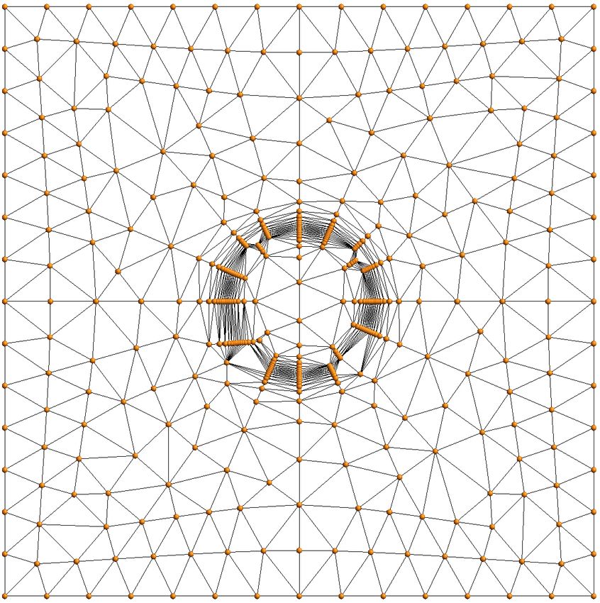
Fig. 4 Sampling of points using toy metric (1) with parameters = 0.01, h = 1/ 10,
1 2
r0 = 0.5 and lmax = 0.3. The square is of size 4 × 4 and is centered at (x , x ) = (0, 0).
choice. Yet, it has the advantage in most cases to generate meshes that are
more structured.
Ensuring that two points are not too close is done using a RTree [2] spatial
search structure. The distance between two points is computed as the shortest
parabola in the given metric (see Equation (3)). Our sampling algorithm
applied to the toy metric (1) provides the set of points of Figure 4.8 Ruili Zhang, Amaury Johnen and Jean-François Remacle
4 Generation of triangles
The set of points optimally sampled are then triangulated using an off the
shelf constrained Delaunay triangulator such as Gmsh [7] or Triangle [12]. We
see on Figure 5 that isotropic straight sided elements are not suited for the
proposed metric. Here, local mesh modifications [10] will be used to align the
mesh with the desired metric. We do not move the points that are optimally
sampled. Only edge swaps will be performed, yet in a non usual fashion.
Fig. 5 Constrained Delaunay mesh constructed using sampled points of Figure 4. The
triangulation is straight sided. It has been done using no specific metric and is thus clearly
not adapted.
High order points are initially placed on every edge of the straight
sided mesh using Equation (3). Assume two triangles t1 (x1 , x2 , x4 ) and
t2 (x2 , x1 , x3 ) that share an edge e (see Figure 6). Triangles t1 and t2 are
possibly curvilinear (as in the Figure) and we aim at evaluating the oppor-
tunity of replacing edge e by edge e0 (edge e0 is the geodesic between x3 and
x4 ). Two indicators will help us to decide whether an edge swap should be
performed:
• The new curvilinear triangles t01 (x4 , x3 , x2 ) and t01 (x3 , x4 , x1 ) have to be
both valid. The validity criterion that is used is based on robust estimates
that have been developed in [8]. In short, for t01 , determinants of jacobians
J4 ,J3 ,J2 ,J43 ,J32 ,J24 are computed at its 6 nodes. A sufficient condition
for triangle t01 to be valid is
J4 > 0 , J3 > 0 , J2 > 0 , 4J43 > J3 +J4 , 4J32 > J3 +J2 , 4J24 > J2 +J4 .
• The quality of the mesh has to be improved by the swap:Curvilinear mesh adaptation 9
min(qg (t1 ), qg (t2 )) < min(qg (t01 ), qg (t02 ))
where qg (t) is a curvilinear quality measure of triangle t with respect to
metric field g.
x3
x23
e0
x13
x34
x2
x12
x24
e
x14
x1 x4
Fig. 6 Curvilinear edge swap.
The quality measure that is used here is a direct extension to standard
quality measures defined in [11]. We define
R √
12 det g dx
qg (t) = √ 2 t (4)
3 Le1 + L2e2 + L2e3
where e1 , e2 and e3 are the three edges of t, Le is the length of e with
respect to the metric. Note that triangle inequality is not necessary verified in
Riemannian metrics i.e. Le1 ≤ Le2 +Le3 is not necessary true. In consequence,
quality measure qg (t) may be larger than one. Edges are swapped until a
stable configuration is found.10 Ruili Zhang, Amaury Johnen and Jean-François Remacle 5 Examples 5.1 Unit mesh for the toy metric Figure 7 present meshes for the toy metric (1). All triangles are valid by construction. Fig. 7 Curvilinear mesh of the unit square using the toy metric. Note here that the corresponding P 1 mesh of our P 2 mesh is totally invalid. It is indeed not possible to generate a P 1 mesh and curving it afterwards without doing curvilinear local mesh modifications (see Figure 8). In the sampling process, points are placed along true geodesics while edges of the mesh are parabola. Parabola that have the same endpoints as true unit geodesics could potentially be longer than 1. Even though the number of long edges that are the consequence of this approximation is quite small, this discrepancy could potentially become annoying. We have addressed that issue by reducing the size of geodesics with the aim at producing parabolas that are of the right unit size. With this fix, edge lengths are in the range [0.701, 1.66] which is very close to the optimal range (see Figure 9). Note that no short edges can exist in the mesh by construction. Long edges are due to the inability of the swapping process to connect points that are close enough without generating invalid P 2 triangles. In further work, other mesh optimizations will be put into place that could enhance even further the quality of the P 2 meshes. Quality measures (4) are also depicted in Figure 9.
Curvilinear mesh adaptation                                                            11

Fig. 8 This Figure depicts the corresponding P 1 straight sided version of the curvilinear
mesh of Figure 7. A large amount of the P 1 triangles are invalid while every single P 2
triangle of Figure 7 is valid.

Fig. 9 Left Figure shows adimensional lengths of edges of the mesh for the toy metric.
Right Figure present P 2 triangle quality measures (4).
12                              Ruili Zhang, Amaury Johnen and Jean-François Remacle

5.2 Intersection of three toy metrics

Fig. 10 Curvilinear mesh of the unit square using the intersection of three toy metrics.

   This example consist in placing three toy metrics M1 , M2 and M3 in the
4 × 4 square, centered at different locations with different mesh sizes and
intersecting them [6]:
                           M = M1 ∩ M2 ∩ M3 .
Meshes are presented in Figure 10. A total of 1270 mesh vertices were inserted
in the unit square. Then, 840 curvilinear swaps were performed to produce
the final mesh. Edges of the mesh have sizes that are in the range [0.7, 1.8].

5.3 Other analytical metrics

We have used our technique to adapt to iso zero of two functions (Figure 11
and Figure 12). Our procedure seems to remain stable and robust for thicker
and thiner adaptations.

6 Conclusions

In this paper, a new methodology for generating unit curvilinear meshes has
been proposed. The method guarantees two important properties in the final
mesh:
Curvilinear mesh adaptation 13 Fig. 11 Curvilinear mesh adapted to capture (x1 )4 + (x2 )4 = R4 . Fig. 12 Curvilinear mesh adapted to capture (x1 )2 + 2(x2 )4 = R4 . 1. Generated meshes are valid. This importrant property is due to the fact that P2 meshes are valid at any point of the algorithm. The initial mesh is curved along geodesic. A backtracking step is applied to ensure that every triangle of the mesh is valid. Then, edge swaps are only applied if elements are valid. Note that the validity criterion that is used is robust. 2. No short edges will be exist in the mesh. A spatial search procedure is used for ensuring that any point that is inserted is not to close in the sense of geodesics than any other point. This work is now being extended to true adaptation i.e. adapting a mesh to a given function f (x1 , x2 ). Even though metrics are still the right tool for driving mesh adaptation at higher orders, basing g on hessians of f is not correct anymore for higher orders of approximation. Our future work will be to build metric fields that are suited for high order.
14                              Ruili Zhang, Amaury Johnen and Jean-François Remacle

Acknowledgements This research is supported by the European Research Council
(project HEXTREME, ERC-2015-AdG-694020) and by the Fond de la Recherche Sci-
entifique de Belgique (F.R.S.-FNRS).

References

 1. Tristan Carrier Baudouin, Jean-François Remacle, Emilie Marchandise, François Hen-
    rotte, and Christophe Geuzaine. A frontal approach to hex-dominant mesh generation.
    Advanced Modeling and Simulation in Engineering Sciences, 1(1):8, 2014.
 2. Norbert Beckmann, Hans-Peter Kriegel, Ralf Schneider, and Bernhard Seeger. The r*-
    tree: an efficient and robust access method for points and rectangles. In Acm Sigmod
    Record, volume 19, pages 322–331. Acm, 1990.
 3. P-E Bernard, J-F Remacle, and Vincent Legat. Boundary discretization for high-
    order discontinuous galerkin computations of tidal flows around shallow water islands.
    International Journal for Numerical Methods in Fluids, 59(5):535–557, 2009.
 4. Bernardo Cockburn and Chi-Wang Shu. Tvb runge-kutta local projection discon-
    tinuous galerkin finite element method for conservation laws. ii. general framework.
    Mathematics of computation, 52(186):411–435, 1989.
 5. Alexandre Ern and Jean-Luc Guermond. Theory and practice of finite elements,
    volume 159. Springer Science & Business Media, 2013.
 6. Pascal-Jean Frey and Frédéric Alauzet. Anisotropic mesh adaptation for cfd computa-
    tions. Computer methods in applied mechanics and engineering, 194(48-49):5068–5082,
    2005.
 7. Christophe Geuzaine and Jean-François Remacle. Gmsh: A 3-d finite element mesh
    generator with built-in pre-and post-processing facilities. International journal for
    numerical methods in engineering, 79(11):1309–1331, 2009.
 8. Amaury Johnen, J-F Remacle, and Christophe Geuzaine. Geometrical validity of
    curvilinear finite elements. Journal of Computational Physics, 233:359–372, 2013.
 9. Norbert Kroll. The adigma project. In ADIGMA-A European Initiative on the De-
    velopment of Adaptive Higher-Order Variational Methods for Aerospace Applications,
    pages 1–9. Springer, 2010.
10. Xiangrong Li, Mark S Shephard, and Mark W Beall. 3d anisotropic mesh adaptation by
    mesh modification. Computer methods in applied mechanics and engineering, 194(48-
    49):4915–4950, 2005.
11. Jonathan Shewchuk. What is a good linear finite element? interpolation, conditioning,
    anisotropy, and quality measures (preprint). University of California at Berkeley,
    73:137, 2002.
12. Jonathan Richard Shewchuk. Triangle: Engineering a 2d quality mesh generator and
    delaunay triangulator. In Applied computational geometry towards geometric engi-
    neering, pages 203–222. Springer, 1996.
13. Jeffrey Slotnick, Abdollah Khodadoust, Juan Alonso, David Darmofal, William Gropp,
    Elizabeth Lurie, and Dimitri Mavriplis. Cfd vision 2030 study: a path to revolutionary
    computational aerosciences. 2014.
You can also read