Data Mining Input: Concepts, Instances, and Attributes
←
→
Page content transcription
If your browser does not render page correctly, please read the page content below
1/28/2021
Data Mining Input:
Concepts, Instances, and
Attributes
Chapter 2 of Data Mining
Terminology
Components of the input:
Concepts: kinds of things that can be learned
Goal: intelligible and operational concept description
E.g.: “Under what conditions should we play?”
This concept is located somewhere in the input data
Instances: the individual, independent examples of
a concept
Note: more complicated forms of input are possible
Attributes: measuring aspects of an instance
We will focus on nominal and numeric attributes
2
11/28/2021
What is a concept?
Styles of learning:
Classification learning:
understanding/predicting a discrete class
Association learning:
detecting associations between features
Clustering:
grouping similar instances into clusters
Numeric estimation:
understanding/predicting a numeric quantity
Concept: thing to be learned
Concept description:
output of learning scheme
3
Classification learning
Example problems: weather data, medical
diagnosis, contact lenses, irises, labor negotiations,
etc.
Can you think of others?
Classification learning is supervised
Algorithm is provided with actual outcomes
Outcome is called the class attribute of the example
Measure success on fresh data for which class
labels are known (test data, as opposed to training
data)
In practice success is often measured subjectively
How acceptable the learned description is to a human
user
4
21/28/2021
Association learning
Can be applied if no class is specified and any kind
of structure is considered “interesting”
Difference from classification learning:
Unsupervised
I.e., not told what to learn
Can predict any attribute’s value, not just the class, and
more than one attribute’s value at a time
Hence: far more association rules than classification rules
Thus: constraints are necessary
Minimum coverage and minimum accuracy
5
Clustering
Finding groups of items that are similar
Clustering is unsupervised
The class of an example is not known
Success often measured subjectively
Sepal length Sepal width Petal length Petal width Type
1 5.1 3.5 1.4 0.2 Iris setosa
2 4.9 3.0 1.4 0.2 Iris setosa
…
51 7.0 3.2 4.7 1.4 Iris versicolor
52 6.4 3.2 4.5 1.5 Iris versicolor
…
101 6.3 3.3 6.0 2.5 Iris virginica
102 5.8 2.7 5.1 1.9 Iris virginica
…
6
31/28/2021
Numeric estimation
Variant of classification learning where the
output attribute is numeric (also called
“regression”)
Learning is supervised
Algorithm is provided with target values
Measure success on test data
Outlook Temperature Humidity Windy Play-time
Sunny Hot High False 5
Sunny Hot High True 0
Overcast Hot High False 55
Rainy Mild Normal False 40
… … … … …
7
Some input terminology
• Each row in a collection of training data is known as an example
or instance.
• Each column is referred to as an attribute.
• The attributes can be divided into two types:
– the output attribute – the one we want to determine/predict
– the input attributes – everything else
input attributes model output attribute
• Example:
rules
fever or
swollen glands diagnosis
tree
headache or…
…
41/28/2021
What’s in an example?
Instance: specific type of example
Thing to be classified, associated, or clustered
Individual, independent example of target concept
Characterized by a predetermined set of attributes
Input to learning scheme: set of independent
instances dataset
Represented as a single relation/flat file
Note difference from relational database
Rather restricted form of input
No relationships between objects/instances
Most common form in practical data mining
9
Example: A family tree
Peter Peggy Grace Ray
= =
M F F M
Steven Graham Pam Ian Pippa Brian
=
M M F M F M
Anna Nikki
F F
10
51/28/2021
Family tree represented as a table
Name Gender Parent1 parent2
Peter Male ? ?
Peggy Female ? ?
Steven Male Peter Peggy
Graham Male Peter Peggy
Pam Female Peter Peggy
Ian Male Grace Ray
Pippa Female Grace Ray
Brian Male Grace Ray
Anna Female Pam Ian
Nikki Female Pam Ian
11
The “sister‐of” relation:
Two versions
First Second Sister of? First Second Sister of?
person person person person
Peter Peggy No Steven Pam Yes
Peter Steven No Graham Pam Yes
… … … Ian Pippa Yes
Steven Peter No Brian Pippa Yes
Steven Graham No Anna Nikki Yes
Steven Pam Yes Nikki Anna Yes
… … … All the rest No
Ian Pippa Yes
… … …
Anna Nikki Yes Closed-world assumption
… … …
Nikki Anna yes
12
61/28/2021
A full representation in one flat file table
First person Second person Sister
of?
Name Gender Parent1 Parent2 Name Gender Parent1 Parent2
Steven Male Peter Peggy Pam Female Peter Peggy Yes
Graham Male Peter Peggy Pam Female Peter Peggy Yes
Ian Male Grace Ray Pippa Female Grace Ray Yes
Brian Male Grace Ray Pippa Female Grace Ray Yes
Anna Female Pam Ian Nikki Female Pam Ian Yes
Nikki Female Pam Ian Anna Female Pam Ian Yes
All the rest No
If second person’s gender = female
and first person’s parent1 = second person’s parent1
then sister-of = yes
13
Generating a flat file
Process of flattening is called “denormalization”
Several relations are joined together to make one
Possible with any finite set of finite relations
More on this in CSC-341
Problematic: relationships without pre-specified
number of objects
“sister of” contains two objects
concept of nuclear-family may be unknown
combinatorial explosion in the flat file
Denormalization may produce spurious regularities
that reflect structure of database
Example: “supplier” predicts “supplier address”
14
71/28/2021
Multi‐instance Concepts
Each individual example comprises a set of instances
multiple instances may relate to the same example
individual instances are not independent
“bag” of instances in training data have same class
All instances are described by the same attributes
One or more instances within an example may be
responsible for its classification
Goal of learning is still to produce a concept description
Examples
multi‐day game activity (the weather data)
classification of computer users as experts or novices
response of users to multiple credit card promotions
performance of a student over multiple classes
15
What’s in an attribute?
Each instance is described by a fixed predefined
set of features, its “attributes”
But: number of relevant attributes may vary
Example: table of transportation vehicles
Possible solution: “irrelevant value” flag
Related problem: existence of an attribute may
depend on value of another one
Example: “spouse name” depends on “married?”
Possible solution: methods of data reduction
Possible attribute types (“levels of measurement”):
Nominal, ordinal, interval and ratio
Simplifies to nominal and numeric 16
81/28/2021
Types of attributes
• Nominal attributes have values that are "names" of categories.
– there is a small set of possible values
attribute possible values
Fever {Yes, No}
Diagnosis {Allergy, Cold, Strep Throat}
Outlook {sunny, overcast, raining}
• In classification learning, the output attribute is always nominal.
• Nominal comes from the Latin word for name
• No relation is implied among nominal values
• No ordering or distance measure
• Can only test for equality
• Numeric attributes have values that come from a range of numbers.
attribute possible values
Body Temp any value in 96.0‐106.0
Salary any value in $15,000‐250,000
– you can order their values (definition of “ordinal” type)
$210,000 > $125,000
98.6 < 101.3
Types of attributes
• What about this one?
attribute possible values
Product Type {0, 1, 2, 3}
• If numbers are used as IDs or names of categories,
the corresponding attribute is actually nominal.
• Note that it doesn't make sense to order the values of
such attributes.
– example: product type 2 > product type 1
doesn't have any meaning
• Also note that some nominal values can be ordinal:
– hot > mild > cool
– young < old
– freshman < sophomore < junior < senior
91/28/2021
Ordinal quantities
Impose order on values
But no distance between values defined
Example:
attribute “temperature” in weather data
Values: “hot” > “mild” > “cool”
Note: addition and subtraction don’t make sense
Example rule:
temperature < hot play = yes
Distinction between nominal and ordinal not always
clear (e.g. attribute “outlook” – is there an
ordering?)
19
Nominal vs. ordinal
Attribute “age” nominal
If age = young and astigmatic = no
and tear production rate = normal
then recommendation = soft
If age = pre-presbyopic and astigmatic = no
and tear production rate = normal
then recommendation = soft
Attribute “age” ordinal
(e.g. “young” < “pre-presbyopic” < “presbyopic”)
If age pre-presbyopic and astigmatic = no
and tear production rate = normal
then recommendation = soft
20
101/28/2021
Attribute types used in practice
Most schemes accommodate just two levels of
measurement:
nominal and numeric, by which we typically only
mean ordinal
Nominal attributes are also called “categorical”,
”enumerated”, or “discrete”
Ordinal attributes are also called “numeric”, or
“continuous”
23
Preparing the input
Denormalization is not the only issue
Problem: different data sources (e.g. sales
department, customer billing department, …)
Differences: styles of record keeping, conventions, time
periods, primary keys, errors
Data must be assembled, integrated, cleaned up
“Data warehouse”: consistent point of access
External data may be required (“overlay data”)
Leads to many potential dataset problems
24
111/28/2021
Missing values
Frequently indicated by out-of-range entries
E.g. -999, “?”
Types: unknown, unrecorded, irrelevant
Reasons:
malfunctioning equipment
changes in experimental design (e.g., new survey questions)
collation of different datasets
measurement not possible
user refusal to answer survey question
Missing value may have significance in itself (e.g.
missing test in a medical examination)
Most schemes assume that is not the case: “missing”
may need to be coded as additional value 25
Inaccurate values
Reason: data has not been collected for the purpose of
mining
Result: errors and omissions that don’t affect original
purpose of data but are critical to mining
E.g. data on hobbies of university students and faculty
Typographical errors in nominal attributes values need
to be checked for consistency
Typographical, measurement, rounding errors in numeric
attributes outliers need to be identified
What facility of Weka did we learn in lab that might be useful here?
Errors may be deliberate
E.g. wrong zip codes
26
121/28/2021
Unbalanced data
• Suppose the diagnosis dataset had 97
instances of allergy, 2 of cold, and 1 of strep
– Consequences?
• Another lesson about raw accuracy
percentages not telling the whole story
– Recall our prior discussion of the importance of
evaluation
• Predicting the majority outcome rarely says
anything interesting about the data
Other problems
Duplicate / redundant data
Instances
Attributes (already discussed: “What’s in an attribute?”)
Stale data
Different formats
131/28/2021
Noise
• Noisy data is meaningless data
– Not useful for prediction
• The term has often been used as a synonym
for corrupt data
• Its meaning has expanded to include any
data that cannot be understood and
interpreted correctly by machines
– unstructured text for example
• Distinguishing signal from noise is the task at
the heart of data mining
• Addressing these issues requires a process of
data cleaning
• Also called pre‐processing, or
• Data wrangling (sometimes)g
141/28/2021
Getting to know the data
Simple visualization tools are very useful
Nominal attributes: histograms
Q: Is the distribution consistent with background
knowledge?
Build hypotheses about which attributes to study
closely
Numeric attributes: graphs
Q: Any obvious outliers?
2-D and 3-D plots show dependencies
Need to consult domain experts
Too much data to inspect? Take a sample!
More complex data viz tools represent an
entire subdiscipline of Computer Science 31
The ARFF format
%
% ARFF file for weather data with some numeric features
%
@relation weather
@attribute outlook {sunny, overcast, rainy}
@attribute temperature numeric
@attribute humidity numeric
@attribute windy {true, false}
@attribute play? {yes, no}
@data
sunny, 85, 85, false, no
sunny, 80, 90, true, no
overcast, 83, 86, false, yes
...
32
151/28/2021
Additional attribute types
ARFF supports string attributes:
@attribute description string
Similar to nominal attributes but list of values is
not pre‐specified
It also supports date attributes:
@attribute today date
Uses the ISO‐8601 combined date and time
format yyyy‐MM‐dd‐THH:mm:ss
33
Sparse data
In some applications most attribute values in a
dataset are zero
word counts in a text categorization problem
product counts in market basket analysis
ARFF supports sparse data
0, 26, 0, 0, 0 ,0, 63, 0, 0, 0, “class A”
0, 0, 0, 42, 0, 0, 0, 0, 0, 0, “class B”
{1 26, 6 63, 10 “class A”}
{3 42, 10 “class B”}
34
161/28/2021
Finding datasets
• Many sources:
– Google’s Public Data Explorer
– UCI Machine Learning Repository
(https://archive.ics.uci.edu/ml/datasets.php)
– FedStats (http://fedstats.sites.usa.gov/)
– U.S. Census Bureau
– UNdata (http://data.un.org/)
– National Space Science Data Center
– Journal of Statistics Education data archive
– KDnuggets dataset repository
– Kaggle.com (feel like winning some money?)
– Search for “dataset” and the subject you’re interested in
– Tools for data scraping from the web
Applied Pre‐Processing
• Review: The Data Mining Process
• Key steps:
– assemble the data in the format needed for data
mining
• typically a text file
• referred to as pre‐processing:
– Major tasks: extraction, integration, transformation, cleaning,
reduction
– perform the data mining
– interpret/evaluate the results
– apply the results
171/28/2021
Why Data Pre‐processing?
• Data in the real world is dirty
• incomplete: lacking attribute values, lacking certain
attributes of interest
– e.g., occupation=“ ”
• noisy: containing errors or outliers, other values that
are not predictive
– e.g., Salary=“‐10”
• inconsistent: containing discrepancies in codes, names,
or values
– e.g., Age=“23” Birthday=“03/07/1998”
– e.g., Was rating “1,2,3”, now rating “A, B, C”
– e.g., discrepancy between duplicate records
Why is Data Dirty?
• Incomplete data (missing values) may come from
– “Not applicable” data value when collected
– Different considerations between the time when the data was
collected and when it is analyzed
– Human/hardware/software problems
• Noisy data (incorrect values) may come from
– Faulty data collection instruments
– Human or computer error at data entry
– Errors in data transmission
• Inconsistent data may come from
– Different data sources (resulting from integration)
– Functional dependency violation (e.g., modify some linked data)
181/28/2021
Why Data Pre‐Processing?
• No quality data, no quality mining results!
• Quality decisions must be based on quality
data
• Data extraction, integration, transformation,
cleaning, and reduction comprises the
majority of the work of building target data
• Data warehouse needs consistent integration
of quality data
Data Extraction
• Ready‐made downloads
– See prior discussion
• Web scraping
– Requires some programming ability
• Web APIs
– I want some data from service X. Does service X have an API?
– Look at the API documentation. Figure out if there is a URL that
retrieves the kind of data you’re looking for.
– Sign up for an API key if one is required.
– Figure out what parameters you need to include in the URL in order to
get the exact data you want.
– Load the URL, parameters included, into your browser. Get back a
response.
– Take the JSON or XML data and unpack it.
191/28/2021
Data Integration
• Combines data from multiple sources into a
coherent store
• In designing a database, we try to avoid
redundancies by normalizing the data
• As a result, the data for a given entity (e.g., a
customer) may be:
– spread over multiple tables
– spread over multiple records within a given table
Data Integration
• Combines data from multiple sources into a
coherent store
• In designing a database, we try to avoid
redundancies by normalizing the data.
• As a result, the data for a given entity (e.g., a
customer) may be:
– spread over multiple tables
– spread over multiple records within a given table
• To prepare for data warehousing and/or data
mining, we often need to denormalize the data.
– multiple records for a given entity a single record
201/28/2021
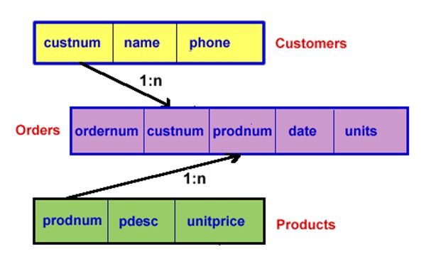
Data Integration
• Example: a simple database design
– Normalized
– Denormalized version would have a single table, with
one instance for every order, with customer and
product information repeated
Data Integration Issues
• Entity identification problem
– identify real world entities from multiple data sources,
e.g., A.cust‐id ≡ B.cust‐#, “LeBron James” vs. “L. James”
• Detecting and resolving data value conflicts
– for the same real world entity, attribute values from
different sources are different
– possible reasons: different representations, different scales
• e.g., metric vs. English units, date formats, etc.
• Redundant data
– Attributes repeated in different databases
– Records with different names in different databases
211/28/2021
Data Integration Issues
• Careful integration of the data from multiple sources may help
reduce/avoid redundancies and inconsistencies and improve
mining speed and quality
• Techniques
– Data scrubbing
• Detect errors and make corrections with simple domain knowledge
– E.g., spell check, zip code knowledge, etc.
– Data auditing
• Analyze data to discover rules and relationships to detect violations
– Clustering to find outliers
– Correlation analysis for redundant attributes
– Numerous others
These fall into the category of data cleaning, coming up.
Transforming the Data
• We may also need to reformat or transform the data
– discretization, normalization are primary examples
– we can use a Python program to do the reformatting
– Weka also provides several useful filters
• One reason for transforming the data: many machine‐
learning algorithms can only handle certain types of
data
221/28/2021
Transforming the Data
• We may also need to reformat or transform the data
– discretization, normalization are primary examples
– we can use a Python program to do the reformatting
– Weka also provides several useful filters
• One reason for transforming the data: many machine‐
learning algorithms can only handle certain types of
data
– some algorithms only work with nominal attributes –
attributes with a specified set of possible values
• examples: {yes, no}
{strep throat, cold, allergy}
– other algorithms only work with numeric attributes
231/28/2021
Discretizing Numeric Attributes
• We can turn a numeric attribute into a
nominal/categorical one by using some sort of
discretization
• This involves dividing the range of possible values
into subranges called buckets or bins.
– example: an age attribute could be divided into these
bins:
child: 0‐12
teen: 12‐17
young: 18‐35
middle: 36‐59
senior: 60‐
Simple Discretization Methods
• What if we don't know which subranges make
sense?
• Equal‐width binning divides the range of possible
values into N subranges of the same size.
– bin width = (max value – min value) / N
– example: if the observed values are all between 0‐
100, we could create 5 bins as follows:
width = (100 – 0)/5 = 20
241/28/2021
Simple Discretization Methods
• What if we don't know which subranges make
sense?
• Equal‐width binning divides the range of possible
values into N subranges of the same size.
– bin width = (max value – min value) / N
– example: if the observed values are all between 0‐
100, we could create 5 bins as follows:
width = (100 – 0)/5 = 20
bins: [0‐20], (20‐40], (40‐60], (60‐80], (80‐100]
[ or ] means the endpoint is included
( or ) means the endpoint is not included
Simple Discretization Methods
• What if we don't know which subranges make
sense?
• Equal‐width binning divides the range of possible
values into N subranges of the same size.
– bin width = (max value – min value) / N
– example: if the observed values are all between 0‐
100, we could create 5 bins as follows:
width = (100 – 0)/5 = 20
bins: [0‐20], (20‐40], (40‐60], (60‐80], (80‐100]
– typically, the first and last bins are extended to allow
for values outside the range of observed values
(‐infinity‐20], (20‐40], (40‐60], (60‐80], (80‐infinity)
251/28/2021
Simple Discretization Methods
• What if we don't know which subranges make
sense?
• Equal‐width binning divides the range of possible
values into N subranges of the same size.
– bin width = (max value – min value) / N
– example: if the observed values are all between 0‐
100, we could create 5 bins as follows:
width = (100 – 0)/5 = 20
bins: [0‐20], (20‐40], (40‐60], (60‐80], (80‐100]
– problems with this equal‐width approach?
Simple Discretization Methods (cont.)
• Equal‐frequency or equal‐height binning divides
the range of possible values into N bins, each of
which holds the same number of training
instances.
– example: let's say we have 10 training examples with
the following values for the attribute that we're
discretizing:
5, 7, 12, 35, 65, 82, 84, 88, 90, 95
261/28/2021
Simple Discretization Methods (cont.)
• Equal‐frequency or equal‐height binning divides
the range of possible values into N bins, each of
which holds the same number of training
instances.
– example: let's say we have 10 training examples with
the following values for the attribute that we're
discretizing:
5, 7, 12, 35, 65, 82, 84, 88, 90, 95
to create 5 bins, we would divide up the range of
values so that each bin holds 2 of the training
examples
Simple Discretization Methods (cont.)
• Equal‐frequency or equal‐height binning divides
the range of possible values into N bins, each of
which holds the same number of training
instances.
– example: let's say we have 10 training examples with
the following values for the attribute that we're
discretizing:
5, 7, 12, 35, 65, 82, 84, 88, 90, 95
To select the boundary values for the bins, this
method typically chooses a value halfway between
the training examples on either side of the boundary
final bins: (‐inf, 9.5], (9.5, 50], (50, 83], (83, 89], (89, inf)
271/28/2021
Simple Discretization Methods (cont.)
• Equal‐frequency or equal‐height binning divides
the range of possible values into N bins, each of
which holds the same number of training
instances.
– example: let's say we have 10 training examples with
the following values for the attribute that we're
discretizing:
5, 7, 12, 35, 65, 82, 84, 88, 90, 95
– Problems with this approach?
Other Discretization Methods
• Ideally, we'd like to come up with bins that
capture distinctions that will be useful in data
mining.
– example: if we're discretizing body temperature,
we'd like the discretization method to learn that
98.6 F is an important boundary value
281/28/2021
Other Discretization Methods
• Ideally, we'd like to come up with bins that
capture distinctions that will be useful in data
mining.
– example: if we're discretizing body temperature,
we'd like the discretization method to learn that
98.6 F is an important boundary value
– more generally, we want to capture distinctions that
will help us to learn to predict/estimate the class of
an example
Other Discretization Methods
• Both equal‐width and equal‐frequency binning
are considered unsupervised methods, because
they don't take into account the class values of
the training examples
291/28/2021
Other Discretization Methods
• Both equal‐width and equal‐frequency binning
are considered unsupervised methods, because
they don't take into account the class values of
the training examples
• There are supervised methods for discretization
that attempt to take the class values into account
– Minimum bucket size
Discretization in Weka
• In Weka, you can discretize an attribute by
applying the appropriate filter to it
• After loading in the dataset in the Preprocess tab,
click the Choose button in the Filter portion of
the tab
301/28/2021
Discretization in Weka
• In Weka, you can discretize an attribute by
applying the appropriate filter to it
• After loading in the dataset in the Preprocess tab,
click the Choose button in the Filter portion of
the tab
• For equal‐width or equal‐height, you choose the
Discretize option in the
filters/unsupervised/attribute folder
– by default, it uses equal‐width binning
– to use equal‐frequency binning instead, click on the
name of the filter and set the useEqualFrequency
parameter to True
Discretization in Weka
• In Weka, you can discretize an attribute by
applying the appropriate filter to it
• After loading in the dataset in the Preprocess tab,
click the Choose button in the Filter portion of
the tab
• For supervised discretization, choose the
Discretize option in the
filters/supervised/attribute folder
311/28/2021
Normalization
• Values scaled to fall within a small, specified
range
• Review: when is this transformation
necessary?
Nominal Attributes with Numeric Values
• Some attributes that use numeric values may
actually be nominal attributes
– the attribute has a small number of possible values
– there is no ordering to the values, and you would
never perform mathematical operations on them
– example: an attribute that uses numeric codes for
medical diagnoses
• 1 = Strep Throat, 2 = Cold, 3 = Allergy
321/28/2021
Nominal Attributes with Numeric Values
• If you load a comma‐separated‐value file containing such an
attribute, Weka will assume that it is numeric
• To force Weka to treat an attribute with numeric values as
nominal, use the NumericToNominal option in the
filters/unsupervised/attribute folder
– click on the name of the filter, and enter the number(s) of the attributes
you want to convert
• Or edit the ARFF file manually…
Data Cleaning
• Fill in missing values,
• smooth noisy data,
• identify or remove outliers,
• correct inconsistent data,
• resolve redundancy caused by data integration
• Importance
– “Data cleaning is the number one problem in data warehousing”
331/28/2021
Handling Missing Values
• Options:
– Ignore them
• PRISM and ID3 won’t work at all
• Naïve Bayes handles them fine
• J48 and nearest neighbor use tricks to get around
– Remove all instances with missing attribute values
• Usually done when the class attribute value is missing
• Unsupervised RemoveWithValues attribute filter in Weka
– Replace missing values with the most common value for
that attribute
• Unsupervised ReplaceMissingValues attribute filter in Weka
• Only works with nominal values
• Issues?
Handling Missing Values
• Options
– Replace with the mean value
– Replace with the mean value for all instances
belonging to the same class (a little smarter for
classification)
– Replace with a new value
• E.g., “unknown”, outlier value to indicate missing (‐999)
– Regression methods for numeric values
• Issues?
341/28/2021
Handing Noisy Data
• Noise:
– random error or variance in a measured attribute
– outlier values
– more generally: non‐predictive values
• Combined computer and human inspection
– detect suspicious values and check by human
– data visualization the key tool
• Clustering
– detect and remove outliers
– also employs data viz
• Regression
– smooth by fitting the data into regression functions
• Binning methods
– employs techniques similar to discretizing
Simple Binning Method
• Sorted attribute values:
4, 8, 9, 15, 21, 21, 24, 25, 26, 28, 29, 34
• Partition into (equal‐depth) bins:
– Bin 1: 4, 8, 9, 15
– Bin 2: 21, 21, 24, 25
– Bin 3: 26, 28, 29, 34
• Smoothing by bin averages:
– Bin 1: 9, 9, 9, 9
– Bin 2: 23, 23, 23, 23
– Bin 3: 29, 29, 29, 29
• Smoothing by bin boundaries:
– Bin 1: 4, 4, 4, 15
– Bin 2: 21, 21, 25, 25
– Bin 3: 26, 26, 26, 34
• Note how smoothing mitigates a noisy/outlier value
351/28/2021
Data Reduction
• Data can be too big to work with
– A database/data warehouse may store terabytes of data
– Complex data analysis/mining may take a very long time to run
on the complete data set
• Data reduction
– Obtain a reduced representation of the data set that is much
smaller in volume but yet produce the same (or almost the
same) analytical results
• Data reduction strategies
– Dimensionality reduction — remove unimportant attributes
– Aggregation and clustering
– Sampling
Dimensionality Reduction
• Feature selection (i.e., attribute subset selection):
– Select a minimum set of attributes (features) that is sufficient
for the data mining task.
• Heuristic methods (due to exponential # of choices):
– step‐wise forward selection
– step‐wise backward elimination
– combining forward selection and backward elimination
– select top N fields using 1R or decision tree algorithm
• rule of thumb: keep top 50 fields
– etc
361/28/2021
Dimensionality Reduction
• Problematic attributes include:
– irrelevant attributes: ones that don't help to predict
the class
• despite their irrelevance, the algorithm may erroneously include
them in the model
Dimensionality Reduction
• Problematic attributes include:
– irrelevant attributes: ones that don't help to predict
the class
• despite their irrelevance, the algorithm may erroneously include
them in the model
– attributes that cause overfitting
• also called false predictors or information leakers
• example: a unique identifier such as Patient ID
371/28/2021
Dimensionality Reduction
• Problematic attributes include:
– irrelevant attributes: ones that don't help to predict
the class
• despite their irrelevance, the algorithm may erroneously include
them in the model
• sometimes want to remove because data is simply too big
– attributes that cause overfitting
• example: a unique identifier such as Patient ID
– redundant attributes: those that offer basically the
same information as another attribute
• example: in many problems, date‐of‐birth and age
provide the same information
• some algorithms may end up giving the information from
these attributes too much weight
Dimensionality Reduction
• Implementation of feature selection (i.e., attribute
subset selection)
• We can remove an attribute manually in Weka by
clicking the checkbox next to the attribute in the
Preprocess tab and then clicking the Remove button
– How to determine?
• Experimentation
• Correlation analysis (filters in Weka)
381/28/2021
Clustering
• Partition data set into clusters, and one can
store cluster representation only
• Can be very effective if data is clustered but
not if data is “smeared”
• There are many choices of clustering
definitions and clustering algorithms. We will
discuss them later
Clustering
391/28/2021
Sampling
• Sampling
– Choose a representative subset of the data
• Simple random sampling may have poor performance in the presence of
skew
– Adaptive sampling methods
• Stratified sampling:
– Approximate the percentage of each class (or subpopulation
of interest) in the overall database
– Used in conjunction with skewed data
Data Reduction
Raw Data Cluster/Stratified Sample
401/28/2021
Undoing pre‐process actions
• In Weka:
– In the Preprocess tab, the Undo button allows you to undo actions
that you perform, including:
• applying a filter to a dataset
• manually removing one or more attributes
– If you apply two filters without using Undo in between the two, the
second filter will be applied to the results of the first filter
– Undo can be pressed multiple times to undo a sequence of actions
Dividing Up the Data File
• To allow us to validate the model(s) learned in
data mining, we'll divide the examples into two
files:
– n% for training
– 100 – n% for testing: these should not be touched
until you have finalized your model or models
– possible splits:
• 67/33
• 80/20
• 90/10
• Alternative to ten‐fold cross validation when you
have a sufficiently large dataset
411/28/2021
Dividing Up the Data File
• You can use Weka to split the dataset for you
after you perform whatever reformatting/editing
is needed
• If you discretize one or more attributes, you need
to do so before you divide up the data file
– otherwise, the training and test sets will be
incompatible
Dividing Up the Data File (cont.)
• Here's one way to do it in Weka:
1) shuffle the examples by choosing the Randomize filter from the
filters/unsupervised/instance folder
2) save the entire file of shuffled examples in Arff format.
3) use the RemovePercentage filter from the same folder
to remove some percentage of the examples
• whatever percentage you're using for the training set
• click on the name of the filter to set the percentage
4) save the remaining examples in a new file
• this will be our test data
5) load the full file of shuffled examples back into Weka
6) use RemovePercentage again with the same percentage
as before, but set invertSelection to True
7) save the remaining examples in a new file
• this will be our training data
421/28/2021
Summary
• Data preparation is a big issue for data mining
• Data preparation includes
– Data extraction (collection, scraping, API, etc.)
– Data integration
– Data transformation (discretization, normalization, etc.)
– Data cleaning
– Data reduction and feature selection
• Many methods have been proposed but still an active
area of research
43You can also read