Data Structures and Tolerant Retrieval - Dr. Goran Glavaš 1 - Universität Mannheim
←
→
Page content transcription
If your browser does not render page correctly, please read the page content below
1

    3. Data Structures and Tolerant Retrieval
                                                       Dr. Goran Glavaš

                                              Data and Web Science Group
                             Fakultät für Wirtschaftsinformatik und Wirtschaftsmathematik
                                                 Universität Mannheim

    CreativeCommons Attribution-NonCommercial-ShareAlike 4.0 International

                                                                                            2.3.2020.
After this lecture, you’ll...
2
Know what data structures are used for implementing inverted index
Understand the pros and cons of hash tables and trees
Know how to handle wildcard queries
Be familiar with methods for handling spelling errors and typos in IR
IR & WS, Lecture 2: Data Structures and Tolerant Retrieval 2.3.2020.Outline
3
Recap of Lecture #2
Data structures for inverted index
Wild-card queries
Spelling correction
IR & WS, Lecture 2: Data Structures and Tolerant Retrieval 2.3.2020.Recap of the previous lecture
4
Boolean retrieval
Q: How are queries represented in Boolean retrieval?
Q: How are documents represented for Boolean retrieval?
Q: How do we find relevant documents for a given query?
Inverted index and finding relevant documents
Q: What is inverted index and what does it consist of?
Q: What are posting lists?
Q: How to merge posting lists?
Q: What is the computational complexity of the merge algorithm?
Q: What are skip pointers and what is their purpose?
Phrase and proximity queries
Q: What is a biword index and what are its shortcomings?
Q: What is a positional index?
Q: How do we use positional index to answer phrase and proximity queries?
IR & WS, Lecture 2: Data Structures and Tolerant Retrieval 2.3.2020.Recap of the previous lecture
5
Inverted index is a data structure for computationally efficient retrieval
Inverted index contains a list of references to documents for all index terms
For each term t we store the list of all documents that contain t
Documents are represented with their identifier numbers (ordinal, starting from 1)
„Frodo” -> [1, 2, 7, 19, 174, 210, 331, 2046]
„Sam” -> [2, 3, 4, 7, 11, 94, 210, 1137]
„blue” -> [2, 3, 24, 2001]
The list of documents that contains a term is called a posting list (or just posting)
Q: Postings are always sorted. Why?
IR & WS, Lecture 2: Data Structures and Tolerant Retrieval 2.3.2020.Recap of the previous lecture
6
So far, we learned how to handle
Regular Boolean queries
Standard merge algorithm over posting lists
Multi-term queries – optimizing according to lengths of posting lists
Phrase queries
Biword index
Positional index
Proximity queries
Positional index
Today we’ll examine
Data structures for implementing the inverted index
How to handle wild-card queries and spelling errors
IR & WS, Lecture 2: Data Structures and Tolerant Retrieval 2.3.2020.Outline
7
Recap of Lecture #2
Data structures for inverted index
Wild-card queries
Spelling correction
IR & WS, Lecture 2: Data Structures and Tolerant Retrieval 2.3.2020.Data structures for inverted index
8
Conceptually, an inverted index is a dictionary
Vocabulary terms (i.e., index terms) are keys
Posting lists are values
„Frodo” -> [1, 2, 7, 19, 174, 210, 331, 2046]
„Sam” -> [2, 3, 4, 7, 11, 94, 210, 1137]
„blue” -> [2, 3, 24, 2001]
But the exact implementation is undefined
What data structures to use?
Where exactly to store different pieces of information – document frequencies,
pointers to posting lists, skip pointers, token positions, ...
IR & WS, Lecture 2: Data Structures and Tolerant Retrieval 2.3.2020.Data structures for inverted index
9
A naïve dictionary – an array of structures
Term Doc. freq. Pointer Each element of the array is a structure
a 656 265 consisting of:
aachen 65 The term itself
The number of documents in the collection in
blue 10 321 which the term appears
... ... ... A pointer to the posting list of the term
Structure size: char[N], int, pointer (int/long)
frodo 221
Q: How to efficiently store the inverted index / dictionary in memory?
Q: How to quickly look up elements at query time?
IR & WS, Lecture 2: Data Structures and Tolerant Retrieval 2.3.2020.Data structures for inverted index
10
Two main choices for implementing the inverted index dictionary
Hash tables
Trees
Both are regularly used in IR systems
Both have advantages and shortcomings
IR & WS, Lecture 2: Data Structures and Tolerant Retrieval 2.3.2020.Inverted index dictionary as a hash table
11
Hash table is a common data structure for implementing dictionaries, i.e., a
structure that maps keys to values as associative arrays
Hash tables rely on hash functions – functions that for a given input value (i.e.,
key) computes the index in the array where the value is stored
Perfect hash function – assigns each key a different index
Most hash functions are imperfect – they may compute the same value for several
different keys – this is called a collision
Q: how to account for collisions?
Each vocabulary term is „hashed” into an integer value
hf(„Frodo”) = 1, hf(„Sam”) = 19, hf(„blue”) = 204
IR & WS, Lecture 2: Data Structures and Tolerant Retrieval 2.3.2020.Inverted index dictionary as a hash table
12
hf(„Frodo”) = 1, hf(„Sam”) = 19, hf(„blue”) = 204, hf(„orc”) = 1
Associative array
1 ... 19 ... 204
„Frodo” -> [1, 2, ..., 2046] „Sam” -> [14, 21, ..., 246] „blue” -> [8, 11, ..., 1132]
„orc” -> [2, 3, ..., 1137]
If the hash function maps the key to the bucket with more than one entry, then
the linear search through the bucket is performed
IR & WS, Lecture 2: Data Structures and Tolerant Retrieval 2.3.2020.Inverted index dictionary as a hash table
13
The main advantage of hash table is fast lookup
Q: What is the complexity of the lookup?
A: O(1)
Shortcomings:
Hash functions are sensitive to minor differences in strings
Close strings not assigned same or close buckets
E.g., hf(„judgment”) = 12, hf(„judgement”) = 354)
As such, they do not support prefix search
Important for tolerant retrieval
Constant vocabulary growth means occasional rehashing for all terms
Q: Why do we need to rehash if the vocabulary grows?
IR & WS, Lecture 2: Data Structures and Tolerant Retrieval 2.3.2020.Inverted index dictionary as a tree
14
Trees divide the vocabulary in the hierarchical form
Each node in the tree captures the subset of the vocabulary
Nodes closer to the root represent larger vocabulary subsets
Nodes closer to leaves encompass narrower subsets
Actual vocabulary terms are found in leaf nodes of the tree
The division of vocabulary is usually alphabetical
Trees should be created in a balanced fashion
Each node in the tree should have approximately the same number of children
Subtrees of nodes of the same depth should have approximately the same number
of leaves
IR & WS, Lecture 2: Data Structures and Tolerant Retrieval 2.3.2020.Inverted index dictionary as a tree
15
root
a-i r-z
j-p
a-cu ge-i j-le ne-p r-so ve-z
cy-ga li-na sp-va
... ... ...
aachen izzard ramstein zygot
IR & WS, Lecture 2: Data Structures and Tolerant Retrieval 2.3.2020.Inverted index dictionary as a tree
16
Q: What is the lookup complexity for a balanced tree with a node degree N which
stores vocabulary containing |V|?
A: Lookup complexity is equal to the depth of the tree, so the complexity is
O(logN|V|)
The central design decision is the degree of the nodes in an index tree, i.e., the
number of child nodes a parent node should have
Large node degree N
Shallow trees, but a large number of children to go through linearly
Small node degree N
Small number of children to linearly search, but deep trees
Advantage
Can handle prefix search
Shortcoming
Lookup complexity (O(logN|V|)) bigger than for hash tables (O(1))
IR & WS, Lecture 2: Data Structures and Tolerant Retrieval 2.3.2020.Outline
17
Recap of Lecture #2
Data structures for inverted index
Wild-card queries
Spelling correction
IR & WS, Lecture 2: Data Structures and Tolerant Retrieval 2.3.2020.Wild-card queries
18
Wild-card queries are queries in which an asterisk sign stands for any sequence
of characters
Wild-card term (with an asterisk) represents a group of terms and not a single term
Trailing wild-card queries (* at the end)
E.g., „mon*” is looking for all documents containing any word beginning with „mon”
Easy to handle with B-tree dictionary: retrieve all words w in range mon ≤ w < moo
Leading wild-card queries (* at the beginning)
E.g., „*mon” is looking for all documents containing any word ending with „mon”
Can be handled with an additional B-tree that indexes vocabulary terms backwards
Retrieve all words w in range: nom ≤ w < non
Q: How to handle queries with the wild-card in the middle?
Retrieve documents containing any word satisfying the wild-card query „co*tion”?
IR & WS, Lecture 2: Data Structures and Tolerant Retrieval 2.3.2020.Wild-card queries
19
Example query
„co*tion” (we want: coordination, comotion, cohabitation, connotation)
Idea:
1. Lookup „co*” in the forward B-tree of the vocabulary
2. Lookup „*tion” in the backward B-tree of the vocabulary
3. Intersect the two obtained term sets
Unfortunately, this is too expensive (too slow) for most real-time IR settings
We need to fetch the relevant documents with a single lookup into index
We need to enrich the index somehow
This will increase the index size, but memory is usually not an issue
IR & WS, Lecture 2: Data Structures and Tolerant Retrieval 2.3.2020.Wild-card queries and permuterm index
20
The idea: besides terms themselves, let’s also index their character-level
permutations
Permuterm index additionally stores permutations of vocabulary terms
We add a special „end-of-term” character ($) and store all permutations:
E.g., „comotion” -> „comotion$”, „n$comotio”, „on$comoti”, „ion$comot”,
„tion$como”, „otion$com”, „motion$co”, „omotion$c”
Q: How to use permuterm index for middle-wild-card queries?
A: Permute the wild-card query until you obtain a trailing query (asterisk at the end)
E.g., „co*tion” -> „co*tion$” -> „tion$co*”
We know how to handle trailing wild-card queries – „tion$co*” can now be handled
by a single permutex index tree
IR & WS, Lecture 2: Data Structures and Tolerant Retrieval 2.3.2020.Wild-card queries and permuterm index
21
Queries supported by permuterm index
Exact queries: for „X” we look up „X$”
Trailing wild-card query: for „X*” we look up „$X*”
Leading wild-card query: for „*X” we look up „X$*”
General wild-card query: for „X*Y” we look up „Y$X*”
Q: How would you handle the query „X*Y*Z” with the permuterm index?
A: Here we have no option but to fire two lookups into the index
1. Retrieve the postings for „X*Z” (by looking up „Z$X*”)
2. Retrieve the posting list for the query „*Y*” (by looking for „Y*”)
3. Merge the two retrieved posting lists
IR & WS, Lecture 2: Data Structures and Tolerant Retrieval 2.3.2020.Character indexes
22
Next idea:
How about we index all character n-grams (sequences of n characters) instead of
whole terms?
We surround all terms with term-boundary symbols and create lists of all sequences
of n consecutive character within terms
Example: „Frodo and Sam fought the orcs” (stopwords removed; lemmatized)
Terms: $frodo$, $sam$, $fight$, $orc$
Char. 3-grams: $fr, fro, rod, odo, do$; $sa, sam, am$; $fi, fig, igh, ght, ht$; $or, orc, rc$
We need to keep the second inverted index
For each character n-gram maintain the list of vocabulary terms that contain it
E.g., „$fr” -> [„freak”, „freedom”, ..., „frodo”, „frozen”]
„sam” -> [„asamoah”, „balsam”, „disambiguate”, ..., „sam”, „subsample”]
IR & WS, Lecture 2: Data Structures and Tolerant Retrieval 2.3.2020.Wild-card queries and character indexes
23
Query for character n-grams and merge results (AND operator)
Example: query „mon*” and 2-gram character indexing
Query is transformed into: „$m” AND „mo” AND „on”
Q: What might be the issue with this transformation?
A: Conjunction of character 2-grams might yield false positives
For example: moon, motivation, moderation, etc.
Compare this issue with the false positives of biword index from Lecture #2
Retrieved terms must be post-filtered against the query to eliminate false positives
Term contains „mon”?
Resulting terms are then looked up in the term-document inverted index
IR & WS, Lecture 2: Data Structures and Tolerant Retrieval 2.3.2020.Character indexes
24
Comparison with permuterm index
Advantage: space efficient (less space needed than for permuterm index)
Shortcoming: slower than using permuterm index
A Boolean query (and term-level merges) needs to be performed for every query term
Wild-card queries in general
Often not supported by Web search engines (not at the character level anyways)
Found in some desktop or library search systems
Wild-cards are conceptually troubling as well
User must know what they don’t know (i.e., where to put the asterisk)
If we have several options in mind, we can just run several concrete queries
IR & WS, Lecture 2: Data Structures and Tolerant Retrieval 2.3.2020.Outline
25
Recap of Lecture #2
Data structures for inverted index
Wild-card queries
Spelling correction
IR & WS, Lecture 2: Data Structures and Tolerant Retrieval 2.3.2020.Spelling correction
26
Primary use-cases for spelling correction
1. Correcting documents during indexing
2. Correcting user queries on-the-fly
Two flavors of spelling correction
1. Isolated words
Check each word on its own for errors in spelling
Will not catch typos that result in another valid word
E.g., „from” „form”
2. Context-sensitive spelling correction
Correctness evaluated by looking at surrounding words as well
E.g., „Frodo went form Gondor to Mordor”
IR & WS, Lecture 2: Data Structures and Tolerant Retrieval 2.3.2020.Document correction
27
Correction should occur prior to indexing
Aiming to have only valid terms in the vocabulary
Smaller vocabulary, i.e., the term dictionary contains fewer entries
We do not change the original documents
Just perform correction when normalizing terms before indexing
Common types of errors for certain types of documents
1. OCR-ed documents – „rn” vs. „m”, „O” vs. „D”
2. Digitally-born documents often have QWERTY keyboard typos – errors from close
keys – „O” vs. „I”, „A” vs. „S”, etc.
IR & WS, Lecture 2: Data Structures and Tolerant Retrieval 2.3.2020.Query correction
28
Primary focus is on correcting errors from queries
Q: Failing to fix errors in queries has more serious consequences than omitting to fix
errors in documents. Why?
With respect to user interface, we have two options
1. Silently retrieving documents according to the corrected query
2. Return several suggested „corrected” query alternatives to the user
„Did you mean?” option
IR & WS, Lecture 2: Data Structures and Tolerant Retrieval 2.3.2020.Isolated word correction
29
The idea: using reference lexicon of correct spellings (i.e., lexicon of valid terms)
Two approaches for obtaining a reference lexicon
1. Existing lexicons like
Standard wide-coverage lexicon of a language (e.g., Webster’s English dictionary)
Domain-specific lexicons (e.g., lexicon of legal terms)
2. Lexicon built from large corpora
E.g., all the words on the web or in Wikipedia
Q: Do we want to keep absolutely all terms from corpora?
IR & WS, Lecture 2: Data Structures and Tolerant Retrieval 2.3.2020.Isolated word correction
30
Given a reference lexicon and the query term (a character sequence from the
query), we do the following:
1. Check if the query term Q is in the reference lexicon
2. If the term Q is not in the reference lexicon, find the entry Q’ from the lexicon that
is „closest” to the query term Q
How do we define „closest”?
We need some similarity/distance measure
We will examine several options
1. Edit distance (also known as Levenshtein distance)
2. Weighted edit distance
3. Character n-gram overlap
IR & WS, Lecture 2: Data Structures and Tolerant Retrieval 2.3.2020.Spelling correction – edit distance
31
Edit distance between two strings S and S’ is the minimal number of operations required
to transform one string into the other
What are the „operations”?
We typically consider operations at the character level
Character insertion („frod” „frodo”)
Character deletion („frpodo” „frodo”)
Character replacement („frido” „frodo”)
Less often: transposition of adjacent characters („fordo” „frodo”)
Transposition equals „deletion” + „insertion”?
Q: Why introducing it as a separate operation?
Levenshtein distance: counts insertions, deletions and replacements
Damerau-Levenshtein distance: additionally counts transpositions as a single operation
Algorithm based on dynamic programming
IR & WS, Lecture 2: Data Structures and Tolerant Retrieval 2.3.2020.Dynamic programming
32
For detailed explanation of dynamic programming see
Cormen, Leiserson, Rivest, and Stein. „Introduction to Algorithms”
Optimal substructure: the optimal solution of the problem contains within itself
the subsolutions, i.e., the optimal solutions to subproblems
Overlapping subsolutions: we can recycle subsolutions – i.e., avoiding repeating
the computation for the same subproblems over and over again
Q: What would be a „subproblem” for the edit distance computation?
A: the edit distance between two prefixes of input strings
Q: Do we have many subproblem repetition for edit distance?
A: most distances between same pair of prefixes are needed 3 times (as a
subproblem of computing distance for insertion, deletion, and substitution)
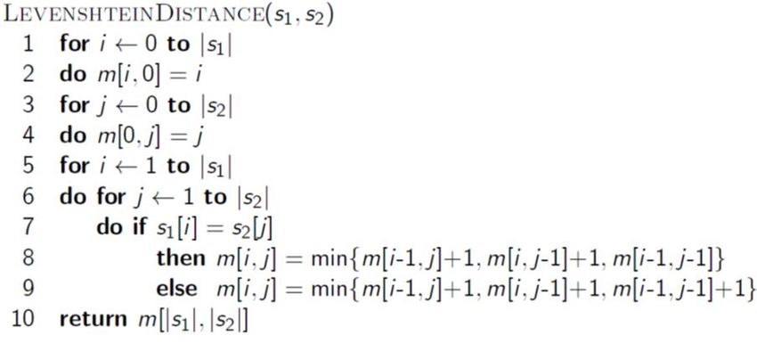
IR & WS, Lecture 2: Data Structures and Tolerant Retrieval 2.3.2020.Levenshtein distance
33
Let a and b be two strings between which we measure edit distance (with |a|
and |b| being their respective lengths):
Mathematically, the Levenshtein distance leva,b(|a|, |b|) is computed as follows:
Where 1(ai ≠ bj) is the indicator function equal to 0 if ai = bj and 1 otherwise
Once we compute leva,b(i, j) for some pair (i, j) we store it in memory so we don’t
compute it again when needed in another recursive thread
Directly implementing this formula requires recursion
IR & WS, Lecture 2: Data Structures and Tolerant Retrieval 2.3.2020.Example – Levenshtein recursively
34
For the example, we will follow only one thread of recursion (first subproblem)
„sany” vs. „sam”
min(lev(„san”, „sam”) + 1, lev(„sany”, „sa”) + 1, lev(„san”, „sa”) + 1)
„san” vs. „sam”
min(lev(„sa”, „sam”) + 1, lev(„san”, „sa”) + 1, lev(„sa”, „sa”) + 1)
„sa” vs. „sam”
min(lev(„s”, „sam”) + 1, lev(„sa”, „sa”) + 1, lev(„s”, „sa”) + 1)
„s” vs. „sam”
min(lev(„”, „sam”) + 1, lev(„s”, „sa”) + 1, lev(„”, „sa”) + 1)
„” vs. „sam”
return 3
IR & WS, Lecture 2: Data Structures and Tolerant Retrieval 2.3.2020.Levenshtein distance – non-recursive version
35
We can avoid the recursion if we start from the recursive algorithm’s end
condition – return max(i, j) if min(i, j) = 0
Then compute the edit distances of larger prefixes from smaller prefixes
IR & WS, Lecture 2: Data Structures and Tolerant Retrieval 2.3.2020.Example – Levenshtein non-recursively
36
_ s a m
_ 0 1 2 3
s 1 0 1 2
a 2 1 0 1
n 3 2 1 1
y 4 3 2 2
IR & WS, Lecture 2: Data Structures and Tolerant Retrieval 2.3.2020.Damerau-Levenshtein distance
37
Standard edit distance counts transposition of adjacent characters as two edits
E.g., „frodo” vs. „fordo”
two character replacements: „r” -> „o” in position 2 and „o” -> „r” in position 3
However, transposing adjacent characters is a single typing error
Damerau-Levenshtein distance introduces transposition as the fourth atomic
distance operation
Q: How would you integrate transposition as a single distance operation into the edit
distance algorithm?
A: d(i,j) additionally needs to consider d(i-2, j-2) + 1(ai-1 = bj & ai = bj-1) when looking
the edit distances of prefixes
IR & WS, Lecture 2: Data Structures and Tolerant Retrieval 2.3.2020.Weighted edit distance
38
Sometimes we want to assign smaller distance to common errors
The weight of an operation (deletion, insertion, replacement, transposition) depends
on the caharcter(s) involved
Motivation: better capture common OCR or typing errors
E.g., On a QWERTY keyboard, letter „m” is much more likely to be mis-typed as „n”
than as „q”
Thus, the replacement operation „m” -> „n” should be assigned smaller edit distance
than „m” -> „q”
Additional input required
Data structure (e.g., weight matrix) containing operation weights for (combinations
of) characters
Q: How to integrate weighting into the edit distance algorithm based on dynamic
programming?
IR & WS, Lecture 2: Data Structures and Tolerant Retrieval 2.3.2020.Using edit distances
39
Given a (misspelled) query we need to find the closest dictionary term
Q: How do we know (or assume) that the query is misspelled in the first place?
A: We don’t find the query term in the vocabulary dictionary
With this strategy, we cannot capture typos like „from” -> „form”
Finding closest dictionary term
Compute edit distance between the query term and each of the dictionary terms?
Too slow (the dictionaries are usually rather large)
We need to somehow pre-filter the „more promising” dictionary entries
IR & WS, Lecture 2: Data Structures and Tolerant Retrieval 2.3.2020.N-gram index for spelling correction
40
Idea: use n-gram index to pre-filter dictionary candidates
1. Enumerate all character n-grams in the query string
E.g., 3-grams in „frodso” -> „fro”, „rod”, „ods”, „dso”
2. Retrieve all vocabulary terms containing any of the obtained character n-grams
Using the inverted index of character n-grams
3. Treshold the obtained list of candidates on the number or percentage of matching
character n-grams
4. Compute the edit distances between the query term and the remaining dictionary
candidates
5. Select the candidate with the smallest edit distance as the correction
IR & WS, Lecture 2: Data Structures and Tolerant Retrieval 2.3.2020.Character n-gram overlap
41
Can be used as
A measure for pre-filtering candidates in order to reduce the number of edit distance
computation
As a self-standing distance measure, alternative to Levenshtein distance
Example
Suppose the query is „fpodo bigginss” and the text is „frodo baggins” and we are
computing the overlap in character 3-grams
{„fpo”, „pod”, „odo”, „big”, „igg”, „ggi”, „ins”, „nss”} vs.
{„fro”, „rod”, „odo”, „bag”, „agg”, „ggi”, „ins”}
We have 3 matching 3-grams: „odo”, „ggi”, and „ins”
That’s 3 out of 8 for the query and 3 out of 7 for the text
Q: What should we take as measure of proximity/distance?
Is raw count of matching n-grams good choice?
IR & WS, Lecture 2: Data Structures and Tolerant Retrieval 2.3.2020.Character n-gram overlap
42
Raw count of matching character n-grams is not a good choice
Does not account for the length of terms in comparison
Two distinct but long terms may have a large raw count of matching n-grams
E.g., „collision” and „collaboration” have 3 matching 3-grams
We need to normalize the score with the length of terms
Jaccard coefficient – a commonly used measure of set overlap
X Y / X Y
Simple alternative: averaged length-normalized overlap
0 .5 X Y / X X Y / Y
IR & WS, Lecture 2: Data Structures and Tolerant Retrieval 2.3.2020.Context-sensitive spelling correction
43
Example:
Suppose the text is „Frodo fled from Mordor back to Gondor”
Suppose the query is „fled form Gondor”
To identify the misspelling „form” -> „from” we need to take into account the
context, i.e., surrounding words
Context-sensitive error correction steps
1. For each term of the query, retrieve dictionary terms that are sufficiently close
„fled” -> {„fled”, „flew”, „flea”}; „form” -> {„form”, „from”}; „gondor” -> {„gondor”}
2. Combine all possibilities (i.e., all combinations of candidates for each term)
„fled form gondor”, „fled from gondor”, „flew form gondor”, „flew from gondor”,
„flea form gondor”, „flea from gondor”,
3. Rank the possibilities according to some criteria
IR & WS, Lecture 2: Data Structures and Tolerant Retrieval 2.3.2020.Context-sensitive spelling correction
44
Hit-based spelling correction
Rank the candidate combinations according to the number of hits (relevant
documents)
Return the candidate with the largest number of hits
Log-based spelling correction
Rank the candidates according to the number of appearances in the query logs (i.e.,
the number of times the same query was posed before)
Useful only if you have a lot of users who fire a lot of queries
Probabilistic spelling correction (e.g., based on language modelling)
Ranking according to probabilities of term sequences
E.g., P(„fled form gondor”) = P(„fled”) * P(„form” | „fled”) * P(„gondor” | „form”)
Often useful to break queries into bigrams:
„fled form gondor” -> „fled form”, „form gondor”
IR & WS, Lecture 2: Data Structures and Tolerant Retrieval 2.3.2020.Now you...
49
Know what data structures you can use for implementing inverted index
Understand the pros and cons of hashtables and trees
Know how to handle wildcard queries
Are familiar with methods for handling spelling errors and typos in IR
IR & WS, Lecture 2: Data Structures and Tolerant Retrieval 2.3.2020.You can also read