ML2014: Higgs Boson Machine Learning Challenge

ML2014: Higgs Boson Machine Learning
                  Challenge
    Jocelyn Perez, Ravi Ponmalai, Alex Silver, Dacoda Strack

 Advisors: Dr. Alexander Ihler, Nick Gallo and Jonathan Stroud

                      University of California, Irvine
                              August 2, 2014

                                   Abstract
         The discovery of the Higgs Boson has been a testament to the co-
     herence of the Standard Model of Physics, but the way in which this
     boson interacts with a fundamental class of particles known as leptons
     has yet to be explored, due to the rarity with which the Higgs Boson
     decays into leptons and the event’s similarity to the decay of other
     particles such as the Z Boson. By creating a machine learning model
     to accurately determine whether a Higgs Boson is decaying into tau
     particles (a type of lepton) within a particle accelerator, physicists
     will be able to explore the nature of the Higgs’s interaction with lep-
     tons. Our model serves to contribute to the work of others involved in
     the Higgs Boson Machine Learning Challenge, a crowdsourced effort
     to generate a satisfactory classification model to be used at CERN’s
     facilities, where the Higgs Boson is studied.

1    Introduction
Machine learning provides a powerful predictive framework to aid in the
process of analyzing large sets of data. In our research, we participate in
Kaggle’s Higgs Boson Machine Learning challenge in an effort to classify
various events in particle physics through the use of machine learning models.

                                       1

2       Kaggle’s Higgs Boson
        Machine Learning Challenge
Kaggle is a website which hosts competitions involving machine learning tasks
posed by businesses or organizations. Past examples of these are the “Greek
Media Monitoring Multilabel Classification” problem, which involved giving
printed media articles searchable keywords automatically and “UPenn and
Mayo Clinic’s Seizure Detection Challenge” which had participants analyze
intracranial EEG data from dogs with epilepsy in order to predict when a
seizure might occur.
    In our case, the goal of the challenge is to determine whether a simu-
lated particle physics event should be classified as “important” (signal) or as
“unremarkable” (background) in the context of a given physics experiment.
    More specifically, we will be going through simulated data generated by
CERN’s ATLAS Project that generates example data from 4 different kinds
particle physics event. The first, our signal, is the tau-tau lepton decay of
a Higgs Boson. This event is interesting because, although the coupling of
the Higgs Boson to bosons (and by extension to fermions) has been explored
and documented/citekaggle, its coupling with leptons is still largely unknown.
Since tau particles are the heaviest and most readily observable of the leptons,
by being able to identify which events involve the Higgs’s decay into tau
particles, we will be opening the way for further research into the nature of
the Higgs Boson.

2.1     Description of the Data
Kaggle provides us with two sets of data: a training set on which to build
our model and a test set whose classifications we predict and that serve to
judge our performance. The training data set consists of 250,000 events,
each containing an ID, a label of signal or background, a weight, and the
measurements of 30 different variables.

2.1.1    Training Data
In order to train our models, we are given a data set that comprises 250,000
simulated particle physics events classified as either signal or background.
Each data point contains 30 features which are either directly measured by
the detector (primitive) or calculated from those measurements (derived). It

                                       2

is worth noting that for some of the data points, the value of certain features
is either not applicable or incalculable and is labelled as missing. In order
to test the accuracy of our models on our local environment, we further
partitioned the training data into two sets of data: 80% training data and
20% validation data. We first provided our models with the training data,
then applied this newly trained model on the validation data. In turn, the
model would return predictions (either signal or background), which could be
compared to their known classifications, allowing us to calculate, by various
metrics, the accuracy of our model.

2.1.2   Test Data
In order to test the models which we have trained, we are further given a
dataset comprised of 550,000 events that lack both signal-background clas-
sification and weight. Otherwise, each data point has the same structure as
the training data, each thirty-featured and with the possibility of missing
measurements.

2.2     Problem Statement
Our focus is to find the most optimal machine learning algorithm configura-
tions to predict whether an event should be classified as “signal” (the tau-tau
lepton decay given off by a Higgs Boson) or as “background” noise (any oth-
erwise unremarkable event) based on the given data collected by the ATLAS
Project.

2.2.1   Motivation
As physics experiments collect larger and larger sets of data, it becomes
unfeasible to sort through the data with an experienced hand and interpret
each datapoint one by one. Just a year of running tests from one experiment
at CERN’s Large Hadron Collider, for example, produces 1 million petabytes
of raw data – something on the order of 20 times the amount of binary data
stored at the US Library of Congress 1 . And astrophysics has similar issues
with the growing amount of raw data collected by their telescopes and other
measuring instruments – the Square Kilometer Array (set to be finished by
   1
     http://www.symmetrymagazine.org/article/august-2012/particle-physics-tames-big-
data

                                         3

2025), for example, is expected to produce more data in one year than exists
on the entire internet today 2 .

2.2.2    Objective
Our objective in this research project will then be to construct a supervised
learning model to perform a binary classification on different events in high
particle physics generated by the ATLAS experiment. With any luck, this
experience will yield some insight into what features of these events hold the
most relevant information, or what features might have the most quirks, and
in doing so lead to more in-depth research into them in the future.

2.3     Background
On July 4, 2012, the discovery of the Higgs boson was announced and con-
firmed six months later. ATLAS 3 had recently observed a signal of the Higgs
boson decaying into two tau particles. In the position of our research group,
no knowledge of particle physics is required to create a reasonable model for
this machine learning task – the only technology necessary is software that
uses simulated data and learns its patterns and behavior.

3       Initial Thoughts
The very first thing we did was attempt to glean information about the data
through histograms of single features and 2-D scatterplots of all possible
combinations of features. At first this was of little use to us, as the amount
of data points and their wide spread made it difficult to discern any useful
pattern.
    2
     http://www.theatlantic.com/technology/archive/2012/04/how-big-data-is-changing-
astronomy-again/255917/
   3
     A particle physics experiment taking place at the Large Hadron Collider at CERN
that searches for new particles and processes using head-on collisions of protons of ex-
traordinarily high energy.

                                           4

4     Our Approaches
4.1    Research Tasks
The very first thing we did was attempt to glean information about the data
through histograms of single features and 2-D scatterplots of all possible
combinations of features. At first this was of little use to us, as the amount
of data points and their wide spread made it difficult to discern any useful
pattern.
    The first model we attempted was the k-nearest neighbors (KNN) model,
as it seemed like a reasonably basic model to start from. K-Nearest Neigh-
bors is a primitive classification model used in machine learning that uses
neighboring data points to draw a conclusion as to the classification of a
given data point. The K represents the size of the neighborhood, or rather
the amount of data points to compare a given data point to in order to clas-
sify it. Since our model’s purpose should be to give a binary classification of
signal or background, K-Nearest Neighbors should logically provide us good
predictions on our data.
                                          v
                                          u n
                                          uX
                       distance(p, q) =   t (q
                                                 i   − pi )2
                                           i=1

Figure 1: The Euclidean Distance formula for measure the distance of two
data points in an n-dimensional space.

    Our K-Nearest Neighbors model uses a Euclidean distance formula (Fig-
ure 1) in a n-dimensional feature space to determine the distance of data
points from one another. Since our data set contains 30 basic features, our
n value is equal to this number of features. This may make it difficult to
determine the nearest data points, especially if we presume that not all of
the features are directly correlated. Our K-Nearest Neighbors model works
best on smaller, correlated data sets with fewer features. With larger data
sets that contain more features, the computation time increases drastically.
    Figure 2 shows the error rate of our predictions of a sample set of only
10,000 points from the training and validation data using this model. As
we steadily increase the number of neighbors that we sample, the error rate
appears to converge on about 20% error rate. This sample test also took
10.75 minutes to compute predictions. On the overall training data alone,

                                      5

Figure 2: This graph compares the error rate of the training and validation
data for the KNN model.

which consists of 250,000 data points, this computation would take 4.5 hours
to make just one prediction set. Due to the constant error rate, limited pa-
rameter functionality and expensive computational time, we did not proceed
further with the K-Nearest Neighbors model.
    We also tested logistic regression models on our data. Logistic Regres-
sion applies a sigmoid function3 to act as a threshold function that outputs
probabilites. We found that this model did not do very well regardless of the
                                          1
                              σ(x) =
                                       1 + e−x

                      Figure 3: The Sigmoid Function

addition of features or changing the model parameters. We believe that one
of the reasons the model performed poorly is because our data had missing
features. In order to compensate for our missing features we would replace
missing values with the median of that feature. We think this adversely
affected the performance of the logistic regression model.

4.1.1   Optimizing Base Models
In order to make the best use of our time we used a few methods to optimize
our code for shorter run times. With the code of one of our mentors we used

                                       6

a method called Iteratively Reweighted Least Squares (IRLS). We used IRLS
to increase the speed at which the gradient descent function finds the optimal
error. Using a boosting method on decision trees is a very computationally

                      Figure 4: The equation for IRLS.

expensive process, to speed this up our mentor wrote a program to convert
the data to an 8 bit unsigned integer(uint8). By using uint8 instead of floating
point values we drastically decreased the time it took to run our code.

4.1.2   Methods used to Evaluate Error
In order to train our models we used different functions to measure our
predictive error. We mainly used loss functions such as mean squared error
to train our models. The mean squared error function uses the validation
data to evaluate how the model would perform on a set of new data.
                                        n
                                     1X
                           M SE =          (Ŷi − Yi )2
                                     n i=1

Figure 5: The mean-squares error function that evaluates a model’s predictive
nature.

4.1.3   Evaluation of Predictions
To evaluate performance of the predictive models Kaggle uses an evalua-
tion metric known as Approximate Median Significance (AMS). This metric
evaluates predictions by taking the false positive and true positive rates into
account. Let s equal the true positive rate and b equal the false positive rate.
    One characteristic of the metric is that false positives are heavily penal-
ized, so in order to mitigate this, all of our soft prediction models had a high
threshold for being classified as the signal class. We also generated a function
that would find a threshold to maximize the AMS score of a given prediction
set, though it was sometimes sensitive to the training set it was associated
with. Cross-validation may have helped us in this regard.

                                       7

s 
                                                   s
                                                            
              AM S =     2 (s + b + 10) log 1 +        −s
                                                b + 10

Figure 6: The AMS formula used to measure accuracy of predictions from a
given model.

4.2    Information Regarding Our Models
To generate our models, we used classes written in MATLAB by the Univer-
sity of California, Irvine’s Alex Ihler which contained all the necessary tools
to generate KNN, decision tree and linear classification models with cluster-
ing. In addition, our boosted tree code was written by Nick Gallo, who also
implemented a binning of the data points such that our calculations would
run somewhere on the order of 100 times faster. To them, we owe a debt of
gratitude. While we also explored Python’s Scikit-learn libraries as packaged
with the Anaconda scientific Python distribution, we were unable to explore
it very deeply due to time restraints.

5     Related Works
Similar work done in this domain include Baldi’s Searching for Exotic Par-
ticles in High-Energy Physics with Deep Learning, in which the researchers
use deep learning in a similar signal-versus-background classification prob-
lem. This method may prove to be a lucrative avenue to explore in the
future, as they showed as much as an 8% increase on their classification
metric through the use of these deep learning techniques[?].

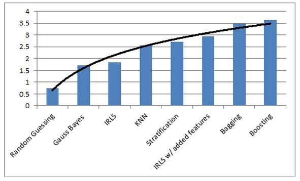
6     Conclusion and Further Work
Through the process of exploring a few models for data analysis we found
that boosting with decision trees was our most effective model.(Figure 7) As
evident in the histogram, more complex models with more manipulability
appeared to yield better results on this feature-driven data set. Due to
the extensive tests and time put into each model taht we tested, we were
unable to test all of the possible machine learning models that would fit
this application. We believe that support vector machines, neural networks,

                                      8

Figure 7: This graph compares the different AMS performances of different
models we tried.

and clustering could perform well on this data set, given the fact that they
are more intellectual models that have more variables that allow for fine-
tuning the results. In addition, other research could be done by looking
deeper into the actual meaning of the features and their associated values.
If their meaning shows a correlation to other data points, then we can more
properly assess the accuracy of a model. Ultimately, finding a model to
accurately detect the presence of the Higgs Boson particle is a difficult task,
but by applying complex machine learning models to the large data set, we
can improve the predictability of this detection.

References
[1] Claire Adam-Bourdarios et. al. Learning to discover: the Higgs boson
    machine learning challenge.

                                      9