Programming with Data - Session 2: R Programming (I) Dr. Wang Jiwei Master of Professional Accounting

Programming with Data
Session 2: R Programming (I)
Dr. Wang Jiwei
Master of Professional Accounting

Introduction to R

What is R?
 R is free and open source
 R is a “statistical programming language”
 Focussed on data handling, calculation, data analysis, and visualization
 R is not a general programming language (wikipedia)
 We will use R for all work in this course

 3 / 72

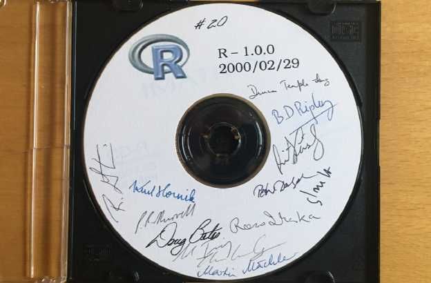
The History of R
 1993: developed by Ross Ihaka and Robert Gentleman at University of
 Auckland
 Why R? "R & R"
 R is written in C and is developed from Bell Laboratory's S language
 2000.2.29: R 1.0.0 official release

 4 / 72

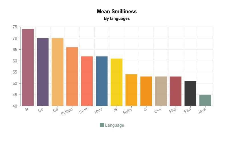
The Happiest R
 based on programmers' pictures on GitHub

 5 / 72

R vs Python
 Each has its own merits

R Python

Statistical analysis with smaller dataset Machine/Deep learning with large dataset
Data visualization General purpose which is great for automation

 6 / 72

Setup
 For this class, I will assume you are using RStudio for R programming. You
 will need to first install R and then RStudio.
 R Installation
 RStudio downloads
 You will need a laptop or desktop for this
 For the most part, everything will work the same across all computer types
 Everything in these slides was tested using R version 4.1.1 (2021-08-10) Kick
 Things on Windows 10 x64 build 18362 

 R and RStudio installation path should be in English. Any non-English
 path may result in installation failure.

 7 / 72

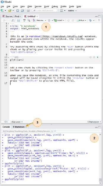
How to use RStudio
1. R markdown file
 integrate code into reports
 more interactive reports with
 analytics
 this slides written with R
 Markdown using the
 xaringan package
2. Console
 Useful for testing code and
 exploring your data
 Enter your code one line at a
 time
3. R Markdown console
 Shows if there are any errors
 when preparing your report

 8 / 72

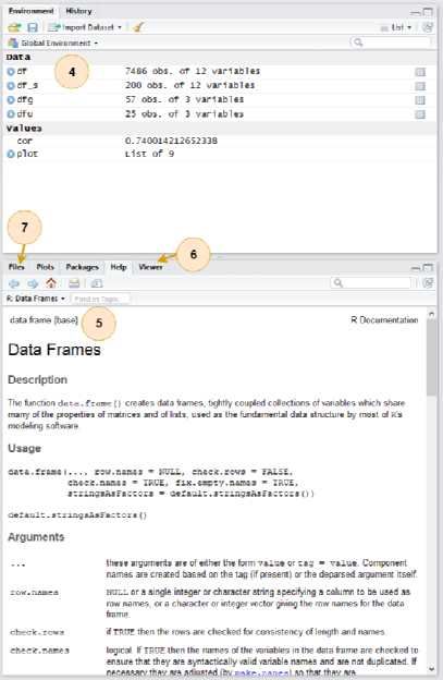
How to use RStudio
4. Environment - Shows all the
 values you have stored
5. Help - Can search documentation
 for instructions on how to use a
 function
6. Viewer - Shows any output you
 have at the moment.
7. Files - Shows files on your
 computer

 9 / 72

Basic R commands

Arithmetic
 Anything in boxes like those on # Addition uses '+'
 the right are R code 1 + 1
 The slides themselves are made in
 R, so you could copy and paste ## [1] 2

 any code in the slides right into R
 # Subtraction uses '-'
 to use it yourself 2 - 1
 Grey boxes: R Code
 Lines starting with hash # are ## [1] 1
 comments
 They only explain what # Multiplication uses '*'
 the code does 3 * 3
 Boxes with ##: Output
 ## [1] 9

 # Division uses '/'
 4 / 2

 ## [1] 2

 11 / 72

Arithmetic
 Exponentiation ^ # Exponentiation uses '^'
 Write x as x ^ y
 y
 5 ^ 5
 Modulus %%
 The remainder after division ## [1] 3125

 Ex.: 46 mod 6 = 4
 25 ^ (1/2)
 1. 6 × 7 = 42
 2. 46 − 42 = 4
 ## [1] 5
 3. 4 < 6, so 4 is the
 remainder # Modulus (remainder) uses '%%'
 Integer division %/% (not used 46 %% 6
 often)
 Like division, but it drops ## [1] 4
 any decimal
 # Integer division uses '%/%'
 46 %/% 6

 ## [1] 7

 12 / 72

Variable assignment
 Variable assignment lets you give # Store 2 in 'x' and 'x1'
 something a name x

Variable assignment
 Note that values are calculated at # Previous value of x and y
 the time of assignment x
 We previously set y

Variable assignment
 To remove a variable, use # Assign value to x
 function rm() x

Application: Singtel
 Set a variable growth to the amount of Singtel's earnings growth
 percent in 2018

# Data from Singtel's earnings reports, in Millions of SGD
singtel_2017

Recap
 So far, we are using R as a glorified calculator
 The key to using R is that we can scale this up with little effort
 Calculating all public companies' earnings growth isn't much harder than
 calculating Singtel's!

 Scaling this up will give use a lot more value

 We can also leverage functions to automate more complex operations
 There are many functions built in, and many more freely available
 We'll also need ways to read data files and work with collections of numbers

 17 / 72

Working with data in R

Data types in R
 The four main types of data in R:
 Numeric: Any number
 Positive or negative
 With or without decimals
 Boolean/Logical: TRUE or FALSE
 Capitalization matters!
 Shorthand is T and F
 Character: "text in quotes"
 More difficult to work with
 Either single or double quotes although double is recommended
 Factor: Converts text into numeric data
 Categorical data for statistical analysis
 eg, convert Male/Female into numbers to be included in statistical
 analysis

 19 / 72

Data types in R
tech_firm

Data types in R
company_name

Practice: Data types
 This practice is to make sure you understand main data types
 Do Exercise 1 on the following R practice file:
 R Practice

 22 / 72

Scaling up......
 We already have some data entered, but it's only a small amount
 We need to scale this up...
 Vectors using c()!
 Matrices using matrix()!
 Lists using list()!
 Data frames using data.frame()!

 Each of these is covered in the coming slides

 23 / 72

Vectors

Vectors: What are they?
 Remember back to linear algebra...
 Examples:

 1
 ⎛ ⎞
 2
 ⎜ ⎟
 ⎜ ⎟ or (1 2 3 4)
 ⎜3⎟

 ⎝ ⎠
 4

 Vector is a row (or column) of data

 25 / 72

Vector creation
 Vectors are entered using the c() command
 Any data type is fine, but all elements must be the same type

company

Vector has no dimension
 A vector in R can be seen as a "concatenation" (in fact c stands for
 concatenate) of elements of 1 or more of the same data type, indexed
 by their positions and so no dimensions (in a spatial sense), but just a
 continuous index that goes from 1 to the length of the object itself.

 A vector is neither a row vector nor a column vector.
 So R will interpret a vector in whichever way makes the matrix product
 sensible.

 27 / 72

Vector has no dimension
dim(earnings) = c(1, 3) # add dimmensions
earnings

## [,1] [,2] [,3]
## [1,] 12662 21204 4286

dim(earnings) = c(3, 1)
earnings

## [,1]
## [1,] 12662
## [2,] 21204
## [3,] 4286

class(earnings)

## [1] "matrix" "array"

dim(earnings) = NULL # remove dimensions
class(earnings)

## [1] "numeric"

 28 / 72

Special cases for vectors
 Counting between integers using Repeating something
 colon and seq() rep(), e.g.
 :, e.g. 1:5 or 22:500 rep(1,times=10) or
 seq(), e.g. seq(from=0, rep("hi",times=5)
 to=100, by=5)
 rep(1, times=10)
1:5
 ## [1] 1 1 1 1 1 1 1 1 1 1
## [1] 1 2 3 4 5
 rep("hi", times=5)
seq(from=0, to=100, by=5)
 ## [1] "hi" "hi" "hi" "hi" "hi"
## [1] 0 5 10 15 20 25 30 35 40 45 50 55 60 65 70 75 80 85 90
## [20] 95 100

↑ note that [20] means the 20th output

 29 / 72

Vector math
 Works the same as scalars (real numbers), but applies element-wise

 First element with first element,
 Second element with second element,
 ......

earnings # previously defined

## [1] 12662 21204 4286

earnings + earnings # Add element-wise

## [1] 25324 42408 8572

earnings * earnings # multiply element-wise

## [1] 160326244 449609616 18369796

 30 / 72

Vector math
 Can also use 1 vector and 1 scalar

 Scalar is applied to all vector elements

earnings + 10000 # Adding a scalar to a vector

## [1] 22662 31204 14286

10000 + earnings # Order doesn't matter

## [1] 22662 31204 14286

earnings / 1000 # Dividing a vector by a scalar

## [1] 12.662 21.204 4.286

 31 / 72

Vector math
 From linear algebra, you might remember multiplication being a bit different,
 as a dot product. That can be done with %*%

# Dot product: sum of product of elements
earnings %*% earnings # returns a matrix though...

## [,1]
## [1,] 628305656

drop(earnings %*% earnings) # drops excess dimensions

## [1] 628305656

 32 / 72

Vector math
 Other useful functions, length() and sum():

length(earnings) # returns the number of elements

## [1] 3

sum(earnings) # returns the sum of all elements

## [1] 38152

 33 / 72

Naming vectors
 Vectors allow us to include a lot Hard to read:
 of information in one object
 It isn't easy to read though earnings
 We can make things more
 readable by assigning names() ## [1] 12662 21204 4286
 Names provide a way to
 easily work with and Easy to read:
 understand the data
 names(earnings)

Selecting vectors
 Selecting can be done a few ways. Multiple selection:
 By index, such as [1] earnings[c(1,2)]
 By name, such as earnings[1:2]
 ["Google"] earnings[c("Google",
 "Microsoft")]
earnings[1]
 # Each of the above 3 is equivalent
## Google earnings[1:2]
## 12662
 ## Google Microsoft
earnings["Google"] ## 12662 21204

## Google
## 12662

 35 / 72

Combining vectors
 Combining is done using c()

c1

Factor vectors
 Factors in R are stored as a vector of integer values with a corresponding set
 of character values to use when the factor is displayed.
 convert character values into numerical values
 categorical variables in statistical modeling
 Levels of a factor are the unique values of that factor variable
 R is giving each unique value of a factor a unique integer, tying it back to
 the character representation
 Levels can be ordered

 37 / 72

Factor vectors
x

Missing data
 Missing data is represented by NA mean(z)
 in R.
 an element of a vector ## [1] NA
 is.na tests each element of a
 vector for missingness mean(z, na.rm = TRUE)
 NULL is the absence of anyting,
 ie, nothingness ## [1] 4.25
 atomical and cannot exist
 y

Vector example
# Calculating profit margin for all public US tech firms
# 715 tech firms with >1M sales in 2017
summary(earnings_2017) # Cleaned data from Compustat, in $M USD

## Min. 1st Qu. Median Mean 3rd Qu. Max.
## -4307.49 -15.98 1.84 296.84 91.36 48351.00

summary(revenue_2017) # Cleaned data from Compustat, in $M USD

## Min. 1st Qu. Median Mean 3rd Qu. Max.
## 1.06 102.62 397.57 3023.78 1531.59 229234.00

profit_margin

Vector example
# order() to sort and return the index for each element
# head() to output the first few elements
head(order(profit_margin))

## [1] 424 477 612 305 317 625

# These are the worst and best profit margin firms in 2017.
profit_margin[order(profit_margin)][c(1, length(profit_margin))]

## HELIOS AND MATHESON ANALYTIC CCUR HOLDINGS INC
## -13.979602 1.026549

 41 / 72

Practice: Vectors
 This practice explores the ROA of Goldman Sachs, JPMorgan, and Citigroup
 in 2017
 Do Exercise 2 on the following R practice file:
 R Practice

 42 / 72

Matrices

Matrices: what are they?
 Remember back to linear algebra...

 Example:

 1 2 3 4
 ⎛ ⎞

 ⎜5 6 7 8 ⎟
 ⎝ ⎠
 9 10 11 12

 Matrix is a rows and columns of data

 44 / 72

Matrix creation
 Matrices are entered using the matrix() command
 Any data type is fine, but all elements must be the same type

columns

Math with matrices
 Everything with matrices works just like vectors

firm_data + firm_data

## [,1] [,2] [,3]
## [1,] 25324 8572 179900
## [2,] 42408 221710 84508

firm_data / 1000

## [,1] [,2] [,3]
## [1,] 12.662 4.286 89.950
## [2,] 21.204 110.855 42.254

 46 / 72

Math with matrices
 Matrix transposing, A , uses t()
 T

firm_data_T

Matrix naming
 We can name matrix rows and columns, much like we named vector elements
 Use rownames() for rows
 Use colnames() for columns

rownames(firm_data)

Selecting from matrices
 Select using 2 indexes instead of 1:
 matrix_name[rows, columns]
 To select all rows or columns, leave that index blanks

firm_data[2, 3]

## [1] 42254

firm_data[, c("Google","Microsoft")]

## Google Microsoft
## Earnings 12662 4286
## Revenue 21204 110855

firm_data[1, ]

## Google Microsoft Goldman
## 12662 4286 89950

 49 / 72

Combining matrices
 Matrices are combined top to bottom as rows with rbind()

# Preloaded: industry codes as indcode (vector)
# - GICS codes: 40 = Financials, 45 = Information Technology
# - https://en.wikipedia.org/wiki/Global_Industry_Classification_Standard

mat

Combining matrices
 Matrices are combined side-by-side as columns with cbind()

# Preloaded: JPMorgan data as jpdata (vector)

mat

Lists

Lists: what are they?
 Like vectors, but with mixed types
 Generally not something we will create, often returned by analysis functions
 in R
 Such as the linear regression models lm()

model |t|)
## (Intercept) -1.837e+02 4.491e+01 -4.091 4.79e-05 ***
## revenue 1.589e-01 3.564e-03 44.585 < 2e-16 ***
## ---
## Signif. codes: 0 '***' 0.001 '**' 0.01 '*' 0.05 '.' 0.1 ' ' 1
##
## Residual standard error: 1166 on 713 degrees of freedom
## Multiple R-squared: 0.736, Adjusted R-squared: 0.7356
## F-statistic: 1988 on 1 and 713 DF, p-value: < 2.2e-16
 53 / 72

str() will tell us what's in this list

str(model)

## List of 11
## $ call : language lm(formula = earnings ~ revenue, data = tech_df)
## $ terms :Classes 'terms', 'formula' language earnings ~ revenue
## .. ..- attr(*, "variables")= language list(earnings, revenue)
## .. ..- attr(*, "factors")= int [1:2, 1] 0 1
## .. .. ..- attr(*, "dimnames")=List of 2
## .. .. .. ..$ : chr [1:2] "earnings" "revenue"
## .. .. .. ..$ : chr "revenue"
## .. ..- attr(*, "term.labels")= chr "revenue"
## .. ..- attr(*, "order")= int 1
## .. ..- attr(*, "intercept")= int 1
## .. ..- attr(*, "response")= int 1
## .. ..- attr(*, ".Environment")=
## .. ..- attr(*, "predvars")= language list(earnings, revenue)
## .. ..- attr(*, "dataClasses")= Named chr [1:2] "numeric" "numeric"
## .. .. ..- attr(*, "names")= chr [1:2] "earnings" "revenue"
## $ residuals : Named num [1:715] -59.7 173.8 -620.2 586.7 613.6 ...
## ..- attr(*, "names")= chr [1:715] "40" "103" "127" "135" ...
## $ coefficients : num [1:2, 1:4] -1.84e+02 1.59e-01 4.49e+01 3.56e-03 -4.09 ...
## ..- attr(*, "dimnames")=List of 2
## .. ..$ : chr [1:2] "(Intercept)" "revenue"
## .. ..$ : chr [1:4] "Estimate" "Std. Error" "t value" "Pr(>|t|)"
## $ aliased : Named logi [1:2] FALSE FALSE
## ..- attr(*, "names")= chr [1:2] "(Intercept)" "revenue"
## $ sigma : num 1166 54 / 72
## $ df : int [1:3] 2 713 2
## $ r.squared : num 0.736
## $ adj.r.squared: num 0.736
## $ fstatistic : Named num [1:3] 1988 1 713
## ..- attr(*, "names")= chr [1:3] "value" "numdf" "dendf"

Looking into lists
 Lists generally use double square brackets, [[index]]
 Used for pulling individual elements out of a list
 [[c()]] will drill through lists, as opposed to pulling multiple values
 Single square brackets pull out elements as it is
 Double square brackets extract just the element
 For 1 level, we can also use $

model["r.squared"] earnings["Google"]

## $r.squared ## Google
## [1] 0.7360059 ## 12662

model[["r.squared"]] earnings[["Google"]]

## [1] 0.7360059 ## [1] 12662

model$r.squared #Can't use $ with vectors

## [1] 0.7360059

 55 / 72

Practice: Lists
 In this practice, we will explore lists and how to parse them
 Do Exercise 3 on the following R practice file:
 R Practice

 56 / 72

Data frames

Data frames: what?
 Data frames are like a hybrid between lists and matrices

Like a matrix: Like a list:

 2 dimensional like matrices Can have different data types for
 Can access data with [] different columns
 All elements in a column must be Can access data with $
 the same data type

 Think of columns as variables, rows as observations, and data frames
 as the Excel spreadsheet

 58 / 72

Example of a data frame
library(DT) # The library is for including larger collections of data in output
datatable(tech_df[1:20, c("conm","tic","margin")],
 options = list(pageLength = 5), rownames=FALSE)

Show 5 entries Search:
 conm tic margin

 AVX CORP AVX 0.00314245229040611
 BK TECHNOLOGIES BKTI -0.0920421373270719
 ADVANCED MICRO DEVICES AMD 0.00806905610808782
 ASM INTERNATIONAL NV ASMIY 0.613509486149511
 SKYWORKS SOLUTIONS INC SWKS 0.276661006737142

Showing 1 to 5 of 20 entries Previous 1 2 3 4 Next

 59 / 72

How to create a df?
 1. On import of data, usually you will get a data frame
 2. Using the data.frame() function

df

Selecting from df
 Access like a matrix

df[, 1]

## [1] "Google" "Microsoft" "Goldman"

 Access like a list

df$companyName

## [1] "Google" "Microsoft" "Goldman"

df[[1]]

## [1] "Google" "Microsoft" "Goldman"

 All are relatively equivalent. Using $ is generally most natural. Using
 [,] is good for complex references.

 61 / 72

Making new columns
 Suggested method: use $

df$all_zero

Sorting data frames
 To sort a vector, we could use the sort()

sort(df$earnings)

## [1] 4286 12662 21204

 THIS CAN'T SORT DATA FRAMES

 A column of a data frame is fine, but it can't sort the whole thing!

 63 / 72

Sorting data frames
 To sort a data frame, we use the order() function
 It returns the order of each element in increasing value
 1 is the lowest value
 Then we pass the new order like we are selecting elements

ordering

Sorting data frames
 Order can sort by multiple levels
 order(level1, level2, ...), where level_ are vectors or df
 columns

example

Subsetting data frames
 1. We can use the selecting methods from before
 2. We can pass a vector of logical values telling R what to keep
 This is pretty useful!
 3. We can also use subset() function

df[df$tech_firm, ] # Remember the comma!

## companyName earnings tech_firm all_zero revenue margin
## Google Google 12662 TRUE 0 110855 0.1142213
## Microsoft Microsoft 21204 TRUE 0 89950 0.2357310

subset(df, earnings < 20000)

## companyName earnings tech_firm all_zero revenue margin
## Goldman Goldman 4286 FALSE 0 42254 0.1014342
## Google Google 12662 TRUE 0 110855 0.1142213

 66 / 72

Practice: Data frames
 This exercise explores the nature of banks' deposits
 We will see which of Goldman, JPMorgan, and Citigroup have (since
 2010):
 The least of their assets in deposits
 The most of their assets in deposits
 Do Exercise 4 on the following R practice file:
 R Practice

 67 / 72

Summary of Session 2

For next week
 continue with your Datacamp and textbook
 review today's code and pre-read next week's seminar notes
 start the Assignment 1 which is due in two weeks.

 Tentatively, there will be the following progress assessment (30%):

1. Individual Assignment 1, on R Programming Basics
2. Individual Assignment 2, on Regressions
3. Two pop up quizzes

 Individual assignments will be in R Markdown (.rmd) file format

 All sumbissions and feedback are on eLearn. Please pay attention to
 academic integrity.

 69 / 72

R Markdown: A quick guide
 Headers and subheaders start with #, ##, ..., ######
 Code blocks starts with and end with (backticks or grave
 accent)
 By default, all code and figures will show up in the output
 echo=FALSE: don't display code in output document
 results="hide": don't display results in output
 Inline code goes in a block starting with and ending with
 Italic font can be used by putting * or _ around text
 Bold font can be used by putting ** around text
 E.g.: **bold text** becomes bold text
 To render the document, click
 Math can be placed between $ to use LaTeX notation
 E.g. $\frac{revt}{at}$ becomes revt

 at

 Full equations (on their own line) can be placed between $$
 A block quote is prefixed with >
 For a complete guide, see R Studio's R Markdown::Cheat Sheet
 My slides are prepared using the xaringan template
 The assignment is prepared using the tufte style

 70 / 72

R Coding Style Guide
Style is subjective and arbitrary but it is important to follow a generally accepted
style if you want to share code with others. I suggest the The tidyverse style guide
which is also adopted by Google with some modification

 Highlights of the tidyverse style guide:
 File names: end with .R
 Identifiers: variable_name, function_name, try not to use "." as it is
 reserved by Base R's S3 objects
 Line length: 80 characters
 Indentation: two spaces, no tabs (RStudio by default converts tabs to
 spaces and you may change under global options)
 Spacing: x = 0, not x=0, no space before a comma, but always place one
 after a comma
 Curly braces {}: first on same line, last on own line
 Assignment: use 
 Semicolon(;): don't use, I used once for the interest of space
 return(): Use explicit returns in functions: default function return is the
 last evaluated expression
 File paths: use relative file path "../../filename.csv" rather than absolute
 path "C:/mydata/filename.csv". Backslash needs \\

 71 / 72

R packages used in this slide
This slide was prepared on 2021-09-03 from Session_2s.Rmd with R version 4.1.1
(2021-08-10) Kick Things on Windows 10 x64 build 18362 .

The attached packages used in this slide are:
## DT kableExtra knitr
## "0.18" "1.3.4" "1.33"

 72 / 72