Demystifying Orthogonal Monte Carlo and Beyond - NIPS Proceedings
←
→
Page content transcription
If your browser does not render page correctly, please read the page content below
Demystifying Orthogonal Monte Carlo and Beyond

               Han Lin ⇤                      Haoxian Chen ⇤                  Tianyi Zhang
           Columbia University              Columbia University             Columbia University
         hl3199@columbia.edu              hc3136@columbia.edu             tz2376@columbia.edu

               Clement Laroche                           Krzysztof Choromanski
              Columbia University               Google Brain Robotics & Columbia University
            cl3778@columbia.edu                            kchoro@google.com

                                                 Abstract
             Orthogonal Monte Carlo [43] (OMC) is a very effective sampling algorithm im-
             posing structural geometric conditions (orthogonality) on samples for variance
             reduction. Due to its simplicity and superior performance as compared to its Quasi
             Monte Carlo counterparts, OMC is used in a wide spectrum of challenging machine
             learning applications ranging from scalable kernel methods [18] to predictive recur-
             rent neural networks [11], generative models [36] and reinforcement learning [16].
             However theoretical understanding of the method remains very limited. In this pa-
             per we shed new light on the theoretical principles behind OMC, applying theory of
             negatively dependent random variables to obtain several new concentration results.
             As a corollary, we manage to obtain first uniform convergence results for OMCs
             and consequently, substantially strengthen best known downstream guarantees for
             kernel ridge regression via OMCs. We also propose novel extensions of the method
             leveraging theory of algebraic varieties over finite fields and particle algorithms,
             called Near-Orthogonal Monte Carlo (NOMC). We show that NOMC is the first
             algorithm consistently outperforming OMC in applications ranging from kernel
             methods to approximating distances in probabilistic metric spaces.

1       Introduction & Related Work
Monte Carlo (MC) methods are widely applied in machine learning in such domains as: dimen-
sionality reduction [1, 3, 2], scalable kernel methods with random feature maps [34], generative
modeling and variational autoencoders via sliced Wasserstein distances [36], approximating Gaussian
smoothings in Evolutionary Strategies (ES) algorithms for Reinforcement Learning (RL) [16], pre-
dictive recurrent neural networks [11] and more. The theory of MC is rich with various techniques
improving the accuracy of base MC estimators such as: antithetic couplings and importance sampling
[6], variance reduction via carefully designed control variate terms [29, 33] and finally: the vast field
of the so-called Quasi Monte Carlo (QMC) methods [7, 27, 20, 19].
Relatively recently, yet another algorithm which can be combined with most of the aforementioned
approaches, called Orthogonal Monte Carlo (OMC) has been proposed [43]. OMC relies on en-
sembles of mutually orthogonal random samples for variance reduction and turns out to be very
effective in virtually all applications of MC in machine learning involving isotropic distributions
[36, 11, 18, 14, 35]. Providing substantial accuracy improvements over MC baselines, conceptually
simple, and superior to algorithms leveraging QMC techniques, it became one of the most frequently
used techniques in a vast arsenal of MC tools.
OMCs are also much simpler than the class of MC methods based on determinantal point processes
(DPPs) [28]. DPPs provide elegant mechanisms for sampling diverse ensembles, where diversity is
encoded by a kernel. Some DPP-MCs [23, 12, 8] provide stronger theoretical guarantees than base
    ⇤
        equal contribution

34th Conference on Neural Information Processing Systems (NeurIPS 2020), Vancouver, Canada.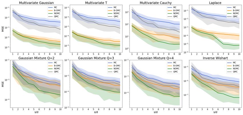
MCs, yet those are impractical to use in higher dimensions due to their prohibitive time complexity,
especially when samples need to be frequently constructed such as in RL [16].
Despite its effectiveness and impact across the field, theoretical principles behind the OMC method re-
main only partially understood, with theoretical guarantees heavily customized to specific applications
and hard to generalize to other settings [35, 14, 17].
In this paper we shed new light on the effectiveness of OMCs by applying theory of negatively
dependent random variables that is a theoretical backbone of DPPs. Consequently, we present
first comprehensive theoretical view on OMCs. Among our new results are first exponentially
small probability bounds for errors of OMCs applied to objectives involving general nonlinear
mappings. Previously such results were known only for the cosine mapping in the setting of
Gaussian kernel approximation via random features [11] and for random linear projections for
dimensionality reduction. Understanding the effectiveness of OMCs in the general nonlinear setting
was considered the Holy Grail of the research on structured MC methods, with elusive general
theory. This striking discrepancy between practice where OMCs are used on a regular basis in general
nonlinear settings and very limited developed theory is one of the main motivations of this work.
Our techniques enable us to settle several open conjectures for OMCs. Those involve not only
aforementioned results for the general nonlinear case, but strong concentration results for arbitrary
RBF kernels with no additional assumptions regarding corresponding spectral densities, in particular
first such results for all Matérn kernels. We show that our concentration results directly imply uniform
convergence of OMCs (which was an open question) and that these lead to substantial strengthening
of the best known results for kernel ridge regression via OMCs from [11]. The strengthenings are
twofold: we extend the scope to all RBF kernels as opposed to just smooth RBFs [11] and we
significantly improve accuracy guarantees.
One of the weaknesses of OMCs is that orthogonal ensembles can be defined only if the number
of samples s satisfies s d, where d stands for data dimensionality. In such a setting a relaxed
version of the method is applied, where one orthogonal block is replaced by multiple independent
orthogonal blocks [43]. Even though orthogonal entanglement of samples across different blocks is
now broken, such block-orthogonal OMC methods (or B-OMCs) were still the most accurate known
MC algorithms for isotropic distributions when s d.
We propose an extension of OMCs relying on the ensembles of random near-orthogonal vectors
preserving entangelements across all the samples, called by us Near-Orthogonal Monte Carlo
(NOMC), that to the best of our knowledge, is the first algorithm beating B-OMCs. Previously,
related ideas are discussed in [37, 10, 30]. [37, 10] summarize different types of energy formulations
and algorithms for distributing points over the sphere, showing that minimizing the discrete Riesz
energy over the sphere S d 1 can produce asymptotically uniformly distributed points. Based on
this, [30] proposes a coordinate descent algorithm to find a local minimum of the discrete Riesz
energy and applies to kernel approximation setting, especially in Gaussian kernel and b-th order
arc-cosine kernels. Motivated by these, we propose an entirely new energy formulation of points over
sphere, and propose a simpler optimization algorithm. In addition, we demonstrate it in different
settings such as: kernel approximation methods (beyond Gaussian and b-th order arc-cosine kernels)
and approximating sliced Wasserstein distances (used on a regular basis in generative modeling).
NOMCs are based on two new paradigms for constructing structured MC samples: high-dimensional
optimization with particle methods and the theory of algebraic varieties over finite fields.
We highlight our main contributions below.
• By leveraging the theory of negatively dependent random variables, we provide first ex-
ponentially small bounds on error probabilities for OMCs used to approximate objectives
involving general nonlinear mappings [Sec. 3: Theorem 1, Theorem 2].
• We show how our general theory can be used to obtain simpler proofs of several known
results and new results not known before [Sec. 2, Sec. 3.1], e.g. first Chernoff-like
concentration inequalities regarding certain classes of Pointwise Nonlinear Gaussian (PNG)
kernels and all RBF kernels (previously such results were known only for RBF kernels with
corresponding isotropic distributions of no heavy tails [15, 11]).
• Consequently, we provide first uniform convergence results for OMCs and as a corollary,
apply them to obtain new SOTA downstream guarantees for kernel ridge regression with
OMCs [Sec. 3.1.1], improving both: accuracy and scope of applicability.
2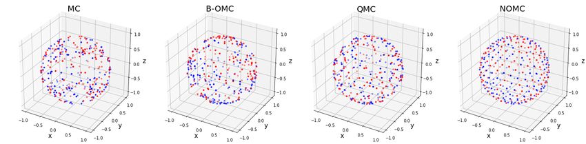
• We propose two new paradigms for constructing structured samples for MC methods when
s d, leveraging number theory techniques and particle methods for high-dimensional
optimization. In particular, we apply a celebrated Weil Theorem [41] regarding generating
functions derived from counting the number of points on algebraic varieties over finite fields.
• We empirically demonstrate the effectiveness of NOMCs [Sec. 5].
2 Orthogonal Monte Carlo
Consider a measurable function fZ : Rd ! Rk parameterized by an ordered subset Z ✓ord Rd with:
def
Ff,D (Z) = E!⇠D [fZ (!)], (1)
where D is an isotropic probability distribution on R (isotropic distribution in this paper is defined
d
as having constant probabilistic density function on every sphere centered at zero). In this work we
analyze MC-based approximation of F . Examples of important machine learning instantiations of F
are given below.
Kernel Functions & Random Features: Every shift-invariant kernel K : Rd ⇥ Rd ! R can
def
be written as K(x, y) = g(x y) = E!⇠D [cos(! > (x y))] for some probability distribution
D [34]. Furthermore, if K is a radial basis function (RBF) kernel (e.g. Gaussian or Matérn),
i.e. K(x, y) = r(kx yk2 ) for some r : R 0 ! R, then D is isotropic. Here Z = (z), where
z = x y, and f(z) (!) = cos(! > z). For pointwise nonlinear Gaussian [PNG] kernels [18] (e.g.
angular or arc-cosine), given as Kh (x, y) = E!⇠N (0,Id ) [h(! > x)h(! > y)], where h : R ! R, the
corresponding distribution D is multivariate Gaussian and f is given as f(x,y) = h(! > x)h(! > y).
Dimensionality Reduction [JLT]: Johnson-Lindenstrauss dimensionality reduction techniques
(JLT) [26, 1, 31] rely on embeddings of high-dimensional feature vectors via random projections
given by vectors ! ⇠ N (0, Id ). Expected squared distances between such embeddings of input
high-dimensional vectors x, y 2 Rd are given as: dist2JLT (x, y) = E!⇠N (0,Id ) [(! > (x y))2 ]. Here
D is multivariate Gaussian and f(z) = (! > z)2 for z = x y.
Sliced Wasserstein Distances [SWD]: Wasserstein Distances (WDs) are metrics in spaces of
probability distributions that have found several applications in deep generative models [5, 24]. For
p 1, the p-th Wasserstein distance between two distributions ⌘ and µ over Rd is defined as:
✓ Z ◆ p1
p
WDp (⌘, µ) = inf ||x y||2 d (x, y) ,
2 (⌘,µ) Rd ⇥Rd
where (⌘, µ) is the set of joint distributions over Rd ⇥ Rd for which the marginal of the first/last
d coordinates is ⌘/µ. Since WD computations involve solving nontrivial optimal transport problem
(OPT) [38] in the high-dimensional space, in practice its more efficient to compute proxies are used,
among them the so-called Sliced Wasserstein Distance (SWD) [9]. SWDs are obtained by constructing
projections ⌘u and µu of ⌘ and µ into a random 1d-subspace encoded by u ⇠ Unif(S d 1 ) chosen
uniformly at random from the unit sphere S d 1 in Rd (see: Sec. 5). If ⌘ and µ are given as point
clouds, they can be rewritten as in Eq. 1, where Z encodes ⌘ and µ via cloud points.
2.1 Structured ensembles for Monte Carlo approximation
A naive way of estimating function Ff,D (Z) from Eq. 1 is to generate s independent samples :
iid
!1iid , ..., !siid ⇠ D, which leads to the base unbiased Monte Carlo (MC) estimator:
Xs
def 1
Fbf,D
iid
(Z) = fZ (!iiid ). (2)
s i=1
Orthogonal Monte Carlo (OMC) method relies on the isotropicity of D and instead entangles different
samples in such a way that they are exactly orthogonal, while their marginal distributions match
those of !iiid (this can be easily done for instance via Gram-Schmidt orthogonalization followed
by row-renormalization, see: [43]). Such an ensemble {!1ort , ..., !sort } is then used to replace
{!1iid , ..., !siid } in Eq. 2 to get OMC estimator Fbf,D
ort
(Z).
Estimator Fbf,D
ort
(Z) can be constructed only if s d, where d stands for samples’ dimensionality. In
most practical applications we have: s > d and thus instead the so-called block orthogonal Monte
3Carlo (B-OMC) procedure is used, where s samples are partitioned into d-size blocks, samples within
each block are chosen as above and different blocks are constructed independently [43]. In B-OMC,
orthogonality is preserved locally within a block, but this entanglement is lost across the blocks.
In the next section we provide new general theoretical results for OMCs.
3 Orthogonal Monte Carlo and Negatively Dependent Ensembles
For a rigorous analysis, we will consider an instantiation of the objective from Eq. 1 of the form:
Ff,D (z) = E!⇠D [f (! > z)] (3)
for z 2 Rd and some measurable function f : R ! R. We consider classes of functions f (u) satisfy:
F1. monotone increasing or decreasing in |u|,
F2. decomposable as f = f + + f , where f + is monotone increasing and f is monotone
decreasing in |u|,
F3. entire (i.e. expressible as Taylor series with infinite radius of convergence, e.g. polynomials).
Remark: As we will see later, for the class F3 the role of f + and f in the analysis is taken by
functions: even[f ]+ and even[f ] , where even[f ] stands for function obtained from f by taking
terms of the Taylor series expansion corresponding to even powers.
Such objectives Ff,D are general enough to cover: dimensionality reduction setting, all RBF kernels,
certain classes of PNG kernels and several statistics regarding neural network with random weights
(see: Sec. 3.1) that we mentioned before. See also Table 1, where we give an overview of specific
examples of functions covered by us, and Sec. 3.1 for much more detailed analysis of applications.
For a random variable X we define moment generating function MX as: MX (✓) = E[e✓X ].
✓a
Furthermore, we define Legendre transform as: LX (a) = sup✓>0 log( MeX (✓) ) if a > E[X] and
✓a
LX (a) = sup✓ 0 for every a 6= E[X].
We prove first exponentially small bounds for failure probabilities of OMCs applied to functions from
all three classes and in addition show that for the class F1 obtained concentration bounds are better
than for the base MC estimator.
Our results can be straightforwardly extended to classes of functions expressible as limits of functions
from the above F1-F3, but for the clarity of the exposition we skip this analysis. To the best of our
knowledge, we are the first to provide theory that addresses also discontinuous functions.
JLT PNG: h(x) = ecx Gaussian ⌫-Matérn
class F1,F3 F3 F2,F3 F2,F3
P1 (cu)2k P1 u4k P1 u4k
f + (u)/even[f ]+ (u) x2 k=0 (2k)! k=0 (4k)! k=0 (4k)!
P1 u4k+2
P1 u4k+2
f (u)/even[f ] (u) N/A N/A k=0 (4k+2)! k=0 (4k+2)!
SOTA results for OMC ortho-JLTs [26] ours [11] ours: any ⌫
Table 1: Examples of particular instantiations of function classes F1-F3 covered by our theoretical results.
The key tool we apply to obtain our general theoretical results is the notion of negative dependence
[ND] [32, 40] that is also used in the theory of Determinantal Point Processes (DPPs) [28]:
Definition 1 (Negative Dependence (ND)). Random variables X1 , . . . , Xn are said to be negatively
dependent if both
\ of the following
Y two inequalities hold\ for any x1 , . . . ,Y
xn 2 R
P( Xi xi ) P(Xi xi ), and P( Xi xi ) P(Xi xi ).
i i i i
We show that certain classes of random variables built on orthogonal ensembles satisfy ND property:
Lemma 1 (ND for OMC-samples and monotone functions). For an isotropic distribution D on Rd
and orthogonal ensemble: !1ort , ..., !dort with !iort ⇠ D, random variables:X1 , ..., Xd defined as:
i z| are negatively dependent for any fixed z 2 R .
Xi = |! ort> d
Lemma 1 itself does not guarantee strong convergence for orthogonal ensembles however is one of
the key technical ingredients that helps us to achieve this goal. The following is true:
4>
Lemma 2. Assume that f is a function from the class F1. Let Xi = f (!iort z) for i = 1, ..., n, and
let be a non-positive (or non-negative)Preal number.
YmThen the following holds:
m
E[e i=1 Xi ] E[e Xi ].
i=1
Note that Lemma 2 lead directly to the following corollary relating iid and orthogonal ensembles:
Corollary 1 (exponentials of OMCs and MCs). Let z 2 Rd and assume that function f : R ! R
is from the class F1. Take an isotropic distribution D on Rd , an ensemble of independent samples
!1iid , ..., !siid and an orthogonal ensemble !1ort , ..., !sort giving rise to base MC estimator Fbf,D
iid
(z) of
> b
E!⇠D [f (! z)] and to its orthogonal version Ff,D (z). Then the following is true for any :
ort
bort (z)
F biid (z)
F
E[e f,D ] E[e f,D ]. (4)
Corollary 1 enables us to obtain stronger concentrations results for OMCs than for base MCs for the
class F1. By combining it with extended Markov’s inequality, we obtain the following:
Theorem 1 (OMC-bounds surpassing MC-bounds for the F1-class). Denote by MSE a mean squared
error of the estimator, by s the number of MC samples used and let X = f (! > z) for ! ⇠ D. Then
under assumptions as in Corollary 1, OMC leads to the unbiased estimator satisfying for ✏ > 0:
P[|Fbf,D
ort
(z) Ff,D (z)| ✏] p(✏), (5)
def
where p(✏) is defined as: p(✏) = exp( sLX (Ff,D (z)+✏)+exp( sLX (Ff,D (z) ✏) for unbounded
def 2
f , and is defined as p(✏) = 2 exp( (b2s✏a)2 ) for bounded f 2 [a, b], which is a standard upper bound
on P[|Fbf,D
iid
(z) Ff,D (z)| ✏]. Furthermore: MSE(Fbf,D ort
(z)) MSE(Fbf,D iid
(z)).
For bounded F1-class, a, b are easy to determine. For instance, in the kernel approximation setting,
most of the kernels are bounded, implying that their non-linear mapping f must be bounded as well.
For functions from F2-class, we simply decompose f into its monotone increasing (f + ) and decreas-
ing (f ) part, apply introduced tools independently to f + and f and use union bound. Finally, if f
is taken from the F3-class, we first decompose it into even[f ] and odd[f ] components, by leaving
only even/odd terms in the Taylor series expansion. We then observe that for isotropic distributions
we have: Fodd[f ],D = 0 (see: Appendix Sec. 9.4), and thus reduce the analysis to that of even[f ]
which is from the F2-class. We conclude that:
Theorem 2 (Exponential bounds for OMCs and F2/F3 classes). Let z 2 Rd and assume that
function f : R ! R is from the class F2 or F3. Then for ✏ > 0:
def
P[|Fbf,D
ort
(z) Ff,D (z)| ✏] p(✏) = u+ + u , (6)
def
where u+/ = exp( sLX +/ (Ff,D (z) + 2✏ ) + exp( sLX +/ (Ff,D (z) ✏
2 ), and X +/ is defined
def def
as: X +/ = f +/ if f is from F2 and as: X +/ = (even[f ])+/ if f is from F3. As before,
def s✏2
in the bounded case we can simplify u+ and u to: u+/ = 2 exp( 2(b+/ a+/ )2
), where
a , b , a , b are lower and upper bounds such that: f 2 [a , b ] and f 2 [a , b ] if f is
+ + + + +
from F2 or (even[f ])+ 2 [a+ , b+ ] and (even[f ]) 2 [a , b ] if f is from F3. Furthermore, if
(even[f ])+ = 0 or (even[f ]) = 0, we can tighten that bound using upper bound from Theorem 1
and thus, establish better concentration bounds than for base MC.
The proofs of all our theoretical results are given in the Appendix.
3.1 Applications
In this section we discuss in more detail applications of the presented results. We see that by taking
f (x) = x2 , we can apply our results to the JLT setting from Sec. 2.
General RBF kernels: Even more interestingly, Theorem 2 enables us to give first strong concen-
tration results for all RBF kernels, avoiding very cumbersome technical requirements regarding tails
of the corresponding spectral distributions (see: [15, 11]). In particular, we affirmatively answer an
open question whether OMCs provide exponential concentration guarantees for the class of Matérn
kernels for every value of the hyperparameter ⌫ ([15]). Theorem 2 can be also directly applied to
obtain strong concentration results regarding kernel ridge regression with OMCs (see: Theorem 2
from [11]) for all RBF kernels as opposed to just smooth RBFs as in [11]. Thus we bridge the gap
between theory (previously valid mainly for Gaussian kernels) and practice (where improvements via
OMCs were reported for RBF kernels across the board [15]).
5First Strong Results for Classes of PNG Kernels: We also obtain first exponentially small upper
bounds on errors for OMCs applied to PNG kernels, which were previously intractable and for which
the best known results were coming from second moment methods [18, 13]. To see this, note that
PNGs defined by nonlinearity h(x) = ecx can be rewritten as functions from the class F3 (with
>
z = x + y), namely: Kh (x, y) = E!⇠N (0,Id ) [ec! (x+y) ] (see: Table 1). Furthermore, by applying
Theorem 2, we actually show that these bounds are better than for the base MC estimator.
3.1.1 Uniform Convergence for OMCs and New Kernel Ridge Regression Results
Undoubtedly, one of the most important applications of results from Sec. 3 are first uniform
convergence guarantees for OMCs which provide a gateway to strong downstream guarantees for
them, as we will show on the example of kernel ridge regression. MSE-results for OMCs from
previous works suffice to provide some pointwise convergence, but are too weak for the uniform
convergence and thus previous downstream theoretical guarantees for OMCs were not practical. The
following is true and implies in particular that OMCs converge uniformly for all RBF kernels :
Theorem 3 (Uniform convergence for OMCs). Let M ✓ Rd be compact with diameter diam(M).
Assume that f has Lipschitz constant Lf . Then under assumptions as in Theorem 1 / 2, for any r > 0:
diam(M) d 2r Lf 2
P[ sup |Fbf,D
ort
(z) Ff,D (z)| ✏] C( ) · p(✏/2) + ( ) , (7)
z2M r ✏
where 2 = E!⇠D [! T !] (i.e. the second moment of D), p is as in RHS of inequality from Theorem 1
/ 2 and C > 0 is a universal constant. In particular, if boundedness conditions from Theorem 1 / 2
L diam(M)
are satisfied, one can take: s = ⇥( ✏d2 log( f ✏ )) to get uniform ✏-error approximation with
dL diam(M)
any constant probability (e.g s = ⇥( ✏d2 log( f ✏ )) for Gaussian kernel for which = d).
We can directly apply these results to kernel ridge regression with an arbitrary RBF via OMCs,
by noting that in the RHS of Theorem 2 from [11] upper-bounding the error, we can drop N 2
multiplicative factor if all points are in the compact set (see: Appendix Sec. 9.7). This term was
added as a consequence of simple union bound, no longer necessary if uniform convergence is
satisfied.
4 Near-Orthogonal Monte Carlo Algorithm
Near-Orthogonal Monte Carlo (or: NOMC) is a new paradigm for constructing entangled MC samples
for estimators involving isotropic distributions if the number of samples required satisfies s > d. We
construct NOMC-samples to make points as evenly distributed on the unit sphere as possible. The
angles between any two samples will be close to orthogonal when d is large (note that they cannot be
exactly orthogonal for s > d since this would imply their linear independence). That makes their
distribution much more uniform than in other methods (see: Fig. 1).
Figure 1: Visual comparison of the distribution of samples for four methods for d = 3 and s = 150. From left
to right: base MC, B-OMC, QMC using Halton sequences and our NOMC. The color of points represent the
direction of sampled vectors, with red for head and blue for tail. We see that NOMC produces most uniformly
distributed samples.
This has crucial positive impact on the accuracy of the estimators applying NOMCs, making them
superior to other methods, as we demonstrate in Sec. 5, and still unbiased.
There are two main strategies that we apply to obtain near-orthogonality surpassing this in QMC
or B-OMC. Our first proposition is to cast sample-construction as an optimization problem, where
near-orthogonal entanglement is a result of optimizing objectives involving angles between samples.
We call this approach: opt-NOMC. Even though such an optimization incurs only one-time additional
cost, we also present alg-NOMC algorithm that has lower time complexity and is based on the theory
of algebraic varieties over finite fields. Algorithm alg-NOMC does not require optimization and in
6practice gives similar accuracy, thus in the experimental section we refer to both simply as NOMC.
Below we discuss both strategies in more detail.
4.1 Algorithm opt-NOMC
The idea of Algorithm opt-NOMC is to force repelling property of the samples/particles (that for the
one-block case was guaranteed by the ND-property) via specially designed energy function.
That energy function achieves lower values for well-spread samples/particles and can be rewritten
as the sum over energies E(!i , !j ) of local particle-particle interactions. There are many good
candidates for E(!i , !j ). We chose: E(!i , !j ) = +k!i !j k2 , where > 0 is a tunable hyper-
2
parameter. We minimize such an energy function on the sphere using standard gradient descent
approach with projections. Without loss of generality, we can assume that the isotropic distribution
D under consideration is a uniform distribution on the sphere Unif(S d 1 ), since for other isotropic
distributions we will only need to conduct later cheap renormalization of samples’ lengths. When
the optimization is completed, we return randomly rotated ensemble, where random rotation is
encoded by Gaussian orthogonal matrix obtained via standard Gram-Schmidt orthogonalization of
the Gaussian unstructured matrix (see: [43]). Random rotations enable us to obtain correct marginal
distributions (while keeping the entanglement of different samples obtained via optimization) and
consequently - unbiased estimators when such ensembles are applied. We initialize optimization
with an ensemble corresponding to B-OMC as a good quality starting point. For the pseudocode of
opt-NOMC, see Algorithm 1 box.
Remark: Note that even though in higher-dimensional settings, such an optimization is more
expensive, this is a one time cost. If new random ensemble is needed, it suffices to apply new
random rotation on the already optimized ensemble. Applying such a random rotation is much
cheaper and can be further sped up by using proxies of random rotations (see: [18]). The time
complexity of Algorithm 1 is O(T N 2 d), where T denotes the number of outer for-loop iterations.
For further discussion regarding the cost of the optimization (see: Appendix: Sec 9.8). Detailed code
implementation is available at https://github.com/HL-hanlin/OMC.
Algorithm 1: Near Orthogonal Monte Carlo: opt-NOMC variant
Input: Parameter , ⌘, T ;
Output: randomly rotated ensemble !i (T ) for i = 1, 2, ..., N ;
(0)
Initialize !i (i = 1, 2, ..., N ) with multiple orthogonal blocks in B-OMC
for t = 0, 1, 2, ..., T 1 do
(t) (t)
Calculate Energy Function E(!i , !j ) = (t) (t) 2 for i 6= j 2 {1, ..., N } ;
+k!i ! j k2
for i = 1, 2, ..., N do P
(t) @ E(!i (t) ,!j (t) )
Compute gradients Fi = i6=j
@!i (t)
;
(t)
Update !i (t+1)
!i (t)
⌘Fi ;
!i (t+1)
Normalize !i (t+1)
k!i (t+1) k2
;
end
end
4.2 Algorithm alg-NOMC
As above, without loss of generality we will assume here that D = Unif(S d 1 ) since, as we
mentioned above, we can obtain samples for general isotropic D from the one for Unif(S d 1 ) by
simple length renormalization. Note that in that setting we can quantify how well the samples from
def
the ensemble ⌦ are spread by computing A(⌦) = max i |!i !j |. It is a standard fact from probability
>
1 1p
theory that for base MC samples A(⌦) = ⇥(r 2 d 2 log(d)) with high probability if the size of ⌦
satisfies: |⌦| = dr and that is the case also for B-OMC. The question arises: can we do better ?
It turns out that the answer is provided by the theory of algebraic varieties over finite fields. Without
loss of generality, we will assume that d = 2p, where p is prime. We will encode samples from our
structured ensembles via complex-valued functions gc1 ,...,cr : Fp ! C, given as
1 2⇡i(cr xr + ... + c1 x)
gc1 ,...,cr (x) = p exp( ), (8)
p p
7where Fp and C stand for the field of residues modulo p and a field of complex numbers respectively
and c1 , ..., cr 2 Fp . The encoding CFp ! Rd is as follows:
def
gc1 ,...,cr (x) ! v(c1 , ..., cr ) = (a1 , b1 , ..., ap , bp )> 2 Rd , (9)
where: gc1 ,...,cr (j 1) = aj + ibj . Using Weil conjecture for curves, one can show [41] that:
Lemma 3 (NOMC via algebraic varieties). If ⌦ = {v(c1 , ..., cr )}c1 ,...,cr 2F(p) 2 S d 1 , then |⌦| =
1
pr , and furthermore A(⌦) (r 1)p 2 .
p
Thus we see that we managed to get rid of the log(d) factor as compared to base MC samples and
consequently, obtain better quality ensemble. As for opt-NOMC, before returning samples, we apply
random rotation to the entire ensemble. But in contrary to opt-NOMC, in this construction we avoid
any optimization, and any more expensive (even one time) computations.
5 Experiments
We empirically tested NOMCs in two settings: (1) kernel approximation via random feature maps
and (2) estimating sliced Wasserstein distances, routinely used in generative modeling [42]. For (1),
we tested the effectiveness of NOMCs for RBF kernels, non-RBF shift-invariant kernels as well as
several PNG kernels. For (2), we considered different classes of multivariate distributions. As we
have explained in Sec. 2, the sliced Wasserstein distance for two distributions ⌘, µ is given as:
1
SWD(⌘, µ) = (Eu⇠Unif(S d 1) [WDpp (⌘u , µu )]) p . (10)
In our experiment we took p = 2. We compared against three other methods: (a) base Monte Carlo
(MC), (b) Quasi Monte Carlo applying Halton sequences (QMC) [7] and block orthogonal MC
(B-OMC). Additional experimental details are in the Appendix (Sec. 9.10). The results are presented
in Fig. 2 and Fig. 3. Empirical MSEs were computed by averaging over k = 450 independent
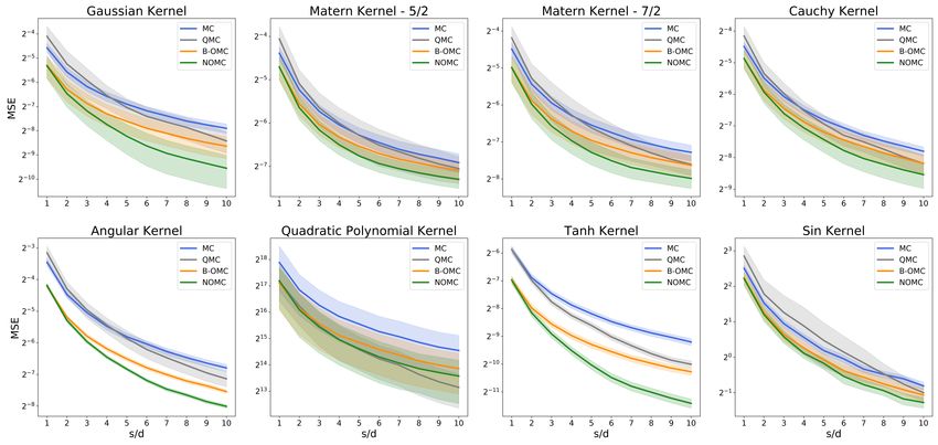
experiments. Our NOMC method clearly outperforms other algorithms. For kernel approximation
NOMC provides the best accuracy for 7 out of 8 different classes of kernels and for the remaining one
it is the second best. For SWD approximation, NOMC provides the best accuracy for all 8 classes of
tested distributions. To the best of our knowledge, NOMC is the first method outperforming B-OMC.
Figure 2: Comparison of MSEs of estimators using different sampling methods: MC, QMC, B-OMC and our
NOMC. First four tested kernels are shift-invariant (first three are even RBFs) and last four are PNGs with name
indicating nonlinear mapping h used (see: Sec. 2). On the x-axis: the number of blocks (i.e. the ratio of the
number of samples D used and data dimensionality d). Shaded region corresponds to 0.5 ⇥ std.
6 Conclusion
In this paper we presented first general theory for the prominent class of orthogonal Monte Carlo
(OMC) estimators (used on a regular basis for variance reduction), by discovering an intriguing
connection with the theory of negatively dependent random variables. In particular, we give first
results for general nonlinear mappings and for all RBF kernels as well as first uniform convergence
guarantees for OMCs. Inspired by developed theory, we also propose new Monte Carlo algorithm
based on near-orthogonal samples (NOMC) that outperforms previous SOTA in the notorious setting,
where number of required samples exceeds data dimensionality.
8Figure 3: As in Fig. 2, but this time we compare estimators of sliced Wasserstein distances (SWDs) between
two distributions taken from a class which name is given above the plot.
7 Broader Impact
General Nonlinear Models: Understanding the impact of structured Monte Carlo methods leverag-
ing entangled ensembles for general nonlinear models is of crucial importance in machine learning
and should guide the research on the developments of new more sample-efficient and accurate MC
methods. We think about our results as a first step towards this goal.
Uniform Convergence Results: Our uniform convergence results for OMCs from Sec. 3.1.1 are the
first such guarantees for OMC methods that can be applied to obtain strong downstream guarantees
for OMCs. We demonstrated it on the example of kernel ridge regression, but similar results can
be derived for other downstream applications such as kernel-SVM. They are important since in
particular they provide detailed guidance on how to choose in practice the number of random features
(see: the asymptotic formula for the number of samples in Theorem 3).
Evolutionary Strategies with Structured MC: We showed the value of our NOMC algorithm in
Sec.5 for kernel and SWD approximation, but the method can be applied as a general tool in several
downstream applications, where MC sampling from isotropic distributions is required, in particular
in evolutionary strategies (ES) for training reinforcement learning policies [16]. ES techniques
became recently increasingly popular as providing state-of-the-art algorithms for tasks of critical
importance in robotics such as end-to-end training of high-frequency controllers [22] as well as
training adaptable meta-policies [39]. ES methods heavily rely on Monte Carlo estimators of gradients
of Gaussians smoothings of certain classes of functions. This makes them potential beneficiaries
of new developments in the theory of Monte Carlo sampling and consequently, new Monte Carlo
algorithms such as NOMC.
Algebraic Monte Carlo: We also think that proposed by us NOMC algorithm in its algebraic variant
is one of a very few effective ways of incorporating deep algebraic results into the practice of MC in
machine learning. Several QMC methods rely on number theory constructions, but, as we presented,
these are much less accurate and in practice not competitive with other structured methods. Not
only does our alg-NOMC provide strong theoretical foundations, but it gives additional substantial
accuracy gains on the top of already well-optimized methods with no additional computational cost.
8 Acknowledgements
We would like to thank Zirui Xu and Ayoujil Jad for their collaboration on putting forward the idea
of opt-NOMC, and thank Noemie Perivier, Yan Chen, Haofeng Zhang and Xinyu Zhang for their
exploration of orthogonal features for downstream tasks.
9 Funding Disclosure
The authors Han Lin, Haoxian Chen, Tianyi Zhang, Clement Laroche are Columbia University
students, and Krzysztof Choromanski works in Google and Columbia University. The work in this
paper is not funded or supported by any third party.
9References
[1] A sparse johnson: Lindenstrauss transform. In L. J. Schulman, editor, Proceedings of the 42nd
ACM Symposium on Theory of Computing, STOC 2010, Cambridge, Massachusetts, USA, 5-8
June 2010, pages 341–350. ACM, 2010.
[2] N. Ailon and B. Chazelle. The fast johnson–lindenstrauss transform and approximate nearest
neighbors. SIAM J. Comput., 39(1):302–322, 2009.
[3] N. Ailon and E. Liberty. An almost optimal unrestricted fast johnson-lindenstrauss transform.
ACM Trans. Algorithms, 9(3):21:1–21:12, 2013.
[4] R. G. Antonini, Y. Kozachenko, and A. Volodin. Convergence of series of dependent '-
subgaussian random variables. Journal of Mathematical Analysis and Applications, 338:1188–
1203, 2008.
[5] M. Arjovsky, S. Chintala, and L. Bottou. Wasserstein generative adversarial networks. In
D. Precup and Y. W. Teh, editors, Proceedings of the 34th International Conference on Machine
Learning, ICML 2017, Sydney, NSW, Australia, 6-11 August 2017, volume 70 of Proceedings of
Machine Learning Research, pages 214–223. PMLR, 2017.
[6] B. Arouna. Adaptative monte carlo method, A variance reduction technique. Monte Carlo Meth.
and Appl., 10(1):1–24, 2004.
[7] H. Avron, V. Sindhwani, J. Yang, and M. W. Mahoney. Quasi-monte carlo feature maps for
shift-invariant kernels. J. Mach. Learn. Res., 17:120:1–120:38, 2016.
[8] R. Bardenet and A. Hardy. Monte carlo with determinantal point processes, 2016.
[9] N. Bonneel, J. Rabin, G. Peyré, and H. Pfister. Sliced and radon wasserstein barycenters of
measures. Journal of Mathematical Imaging and Vision, 51(1):22–45, 2015.
[10] J. S. Brauchart and P. J. Grabner. Distributing many points on spheres: minimal energy and
designs. Journal of Complexity, 31(3):293–326, 2015.
[11] K. Choromanski, C. Downey, and B. Boots. Initialization matters: Orthogonal predictive
state recurrent neural networks. In 6th International Conference on Learning Representations,
ICLR 2018, Vancouver, BC, Canada, April 30 - May 3, 2018, Conference Track Proceedings.
OpenReview.net, 2018.
[12] K. Choromanski, A. Pacchiano, J. Parker-Holder, and Y. Tang. Structured monte carlo sampling
for nonisotropic distributions via determinantal point processes. CoRR, abs/1905.12667, 2019.
[13] K. Choromanski, A. Pacchiano, J. Pennington, and Y. Tang. Kama-nns: Low-dimensional rota-
tion based neural networks. In K. Chaudhuri and M. Sugiyama, editors, The 22nd International
Conference on Artificial Intelligence and Statistics, AISTATS 2019, 16-18 April 2019, Naha,
Okinawa, Japan, volume 89 of Proceedings of Machine Learning Research, pages 236–245.
PMLR, 2019.
[14] K. Choromanski, M. Rowland, W. Chen, and A. Weller. Unifying orthogonal monte carlo
methods. In K. Chaudhuri and R. Salakhutdinov, editors, Proceedings of the 36th International
Conference on Machine Learning, ICML 2019, 9-15 June 2019, Long Beach, California, USA,
volume 97 of Proceedings of Machine Learning Research, pages 1203–1212. PMLR, 2019.
[15] K. Choromanski, M. Rowland, T. Sarlós, V. Sindhwani, R. E. Turner, and A. Weller. The
geometry of random features. In A. J. Storkey and F. Pérez-Cruz, editors, International
Conference on Artificial Intelligence and Statistics, AISTATS 2018, 9-11 April 2018, Playa
Blanca, Lanzarote, Canary Islands, Spain, volume 84 of Proceedings of Machine Learning
Research, pages 1–9. PMLR, 2018.
[16] K. Choromanski, M. Rowland, V. Sindhwani, R. E. Turner, and A. Weller. Structured evolution
with compact architectures for scalable policy optimization. In J. G. Dy and A. Krause,
editors, Proceedings of the 35th International Conference on Machine Learning, ICML 2018,
Stockholmsmässan, Stockholm, Sweden, July 10-15, 2018, volume 80 of Proceedings of Machine
Learning Research, pages 969–977. PMLR, 2018.
10[17] K. Choromanski and V. Sindhwani. Recycling randomness with structure for sublinear time
kernel expansions. In M. Balcan and K. Q. Weinberger, editors, Proceedings of the 33nd
International Conference on Machine Learning, ICML 2016, New York City, NY, USA, June
19-24, 2016, volume 48 of JMLR Workshop and Conference Proceedings, pages 2502–2510.
JMLR.org, 2016.
[18] K. M. Choromanski, M. Rowland, and A. Weller. The unreasonable effectiveness of structured
random orthogonal embeddings. In I. Guyon, U. von Luxburg, S. Bengio, H. M. Wallach,
R. Fergus, S. V. N. Vishwanathan, and R. Garnett, editors, Advances in Neural Information
Processing Systems 30: Annual Conference on Neural Information Processing Systems 2017,
4-9 December 2017, Long Beach, CA, USA, pages 219–228, 2017.
[19] J. Dick and M. Feischl. A quasi-monte carlo data compression algorithm for machine learning.
CoRR, abs/2004.02491, 2020.
[20] J. Dick, F. Y. Kuo, and I. H. Sloan. High-dimensional integration: The quasi-monte carlo way.
Acta Numer., 22:133–288, 2013.
[21] D. Dubhashi and D. Ranjan. Balls and bins: A study in negative dependence. Random Struct.
Algorithms, 13(2):99–124, Sept. 1998.
[22] W. Gao, L. Graesser, K. Choromanski, X. Song, N. Lazic, P. Sanketi, V. Sindhwani, and N. Jaitly.
Robotic table tennis with model-free reinforcement learning. CoRR, abs/2003.14398, 2020.
[23] G. Gautier, R. Bardenet, and M. Valko. On two ways to use determinantal point processes for
monte carlo integration. In H. M. Wallach, H. Larochelle, A. Beygelzimer, F. d’Alché-Buc, E. B.
Fox, and R. Garnett, editors, Advances in Neural Information Processing Systems 32: Annual
Conference on Neural Information Processing Systems 2019, NeurIPS 2019, 8-14 December
2019, Vancouver, BC, Canada, pages 7768–7777, 2019.
[24] I. Gulrajani, F. Ahmed, M. Arjovsky, V. Dumoulin, and A. C. Courville. Improved training of
wasserstein gans. In I. Guyon, U. von Luxburg, S. Bengio, H. M. Wallach, R. Fergus, S. V. N.
Vishwanathan, and R. Garnett, editors, Advances in Neural Information Processing Systems 30:
Annual Conference on Neural Information Processing Systems 2017, 4-9 December 2017, Long
Beach, CA, USA, pages 5767–5777, 2017.
[25] K. Joag-Dev and F. Proschan. Negative association of random variables with applications. The
Annals of Statistics, 11(1):286–295, 1983.
[26] W. B. Johnson and J. Lindenstrauss. Extensions of lipschitz maps into a hilbert space. 1984.
[27] P. Kritzer, H. Niederreiter, F. Pillichshammer, and A. Winterhof, editors. Uniform Distribution
and Quasi-Monte Carlo Methods - Discrepancy, Integration and Applications, volume 15 of
Radon Series on Computational and Applied Mathematics. De Gruyter, 2014.
[28] A. Kulesza and B. Taskar. Determinantal point processes for machine learning. Foundations
and Trends in Machine Learning, 5(2-3):123–286, 2012.
[29] R. Leluc, F. Portier, and J. Segers. Control variate selection for monte carlo integration, 2019.
[30] Y. Lyu. Spherical structured feature maps for kernel approximation. In International Conference
on Machine Learning, pages 2256–2264, 2017.
[31] J. Matousek. On variants of the johnson-lindenstrauss lemma. Random Struct. Algorithms,
33(2):142–156, 2008.
[32] R. Pemantle. Towards a theory of negative dependence. 2000.
[33] F. Portier and J. Segers. Monte carlo integration with a growing number of control variates. J.
Appl. Probab., 56(4):1168–1186, 2019.
[34] A. Rahimi and B. Recht. Random features for large-scale kernel machines. In J. C. Platt,
D. Koller, Y. Singer, and S. T. Roweis, editors, Advances in Neural Information Processing Sys-
tems 20, Proceedings of the Twenty-First Annual Conference on Neural Information Processing
Systems, Vancouver, British Columbia, Canada, December 3-6, 2007, pages 1177–1184. Curran
Associates, Inc., 2007.
11[35] M. Rowland, K. Choromanski, F. Chalus, A. Pacchiano, T. Sarlós, R. E. Turner, and A. Weller.
Geometrically coupled monte carlo sampling. In S. Bengio, H. M. Wallach, H. Larochelle,
K. Grauman, N. Cesa-Bianchi, and R. Garnett, editors, Advances in Neural Information Process-
ing Systems 31: Annual Conference on Neural Information Processing Systems 2018, NeurIPS
2018, 3-8 December 2018, Montréal, Canada, pages 195–205, 2018.
[36] M. Rowland, J. Hron, Y. Tang, K. Choromanski, T. Sarlós, and A. Weller. Orthogonal estimation
of wasserstein distances. In K. Chaudhuri and M. Sugiyama, editors, The 22nd International
Conference on Artificial Intelligence and Statistics, AISTATS 2019, 16-18 April 2019, Naha,
Okinawa, Japan, volume 89 of Proceedings of Machine Learning Research, pages 186–195.
PMLR, 2019.
[37] E. B. Saff and A. B. Kuijlaars. Distributing many points on a sphere. The mathematical
intelligencer, 19(1):5–11, 1997.
[38] F. Santambrogio. Introduction to optimal transport theory, 2010.
[39] X. Song, Y. Yang, K. Choromanski, K. Caluwaerts, W. Gao, C. Finn, and J. Tan. Rapidly
adaptable legged robots via evolutionary meta-learning. CoRR, abs/2003.01239, 2020.
[40] S. Sung. On the exponential inequalities for negatively dependent random variables. Journal of
Mathematical Analysis and Applications - J MATH ANAL APPL, 381:538–545, 09 2011.
[41] A. Weil. Numbers of solutions of equations in finite fields. Bull. Amer. Math. Soc., 55:497–508,
1949.
[42] J. Wu, Z. Huang, D. Acharya, W. Li, J. Thoma, D. P. Paudel, and L. V. Gool. Sliced wasserstein
generative models. In IEEE Conference on Computer Vision and Pattern Recognition, CVPR
2019, Long Beach, CA, USA, June 16-20, 2019, pages 3713–3722. Computer Vision Foundation
/ IEEE, 2019.
[43] F. X. Yu, A. T. Suresh, K. M. Choromanski, D. N. Holtmann-Rice, and S. Kumar. Orthogonal
random features. In D. D. Lee, M. Sugiyama, U. von Luxburg, I. Guyon, and R. Garnett,
editors, Advances in Neural Information Processing Systems 29: Annual Conference on Neural
Information Processing Systems 2016, December 5-10, 2016, Barcelona, Spain, pages 1975–
1983, 2016.
12You can also read