Determination of cloud-top Height through three-dimensional cloud Reconstruction using DIWATA-1 Data - Nature
←
→
Page content transcription
If your browser does not render page correctly, please read the page content below
www.nature.com/scientificreports

            OPEN           Determination of Cloud-top Height
                           through Three-dimensional Cloud
                           Reconstruction using DIWATA-1
                           Data
                           Ellison Castro1,2 ✉, Tetsuro Ishida1 ✉, Yukihiro Takahashi1, Hisayuki Kubota1, Gay Jane Perez2
                           & Joel S. Marciano Jr3,4
                           Cloud-top height is a useful parameter with which to elucidate cloud vertical growth, which
                           often indicates severe weather such as torrential rainfall and thunderstorms; it is widely used in
                           meteorological research. However, general cloud-top height estimation methods are hindered by
                           observational and analytical constraints. This study used data from DIWATA-1, the Philippines’ first
                           microsatellite, to overcome these limitations and successfully produce sophisticated three-dimensional
                           cloud models via stereo-photogrammetry. High-temporal snapshot 200-ms-interval imaging of clouds
                           over Iloilo, Philippines, is performed. Two types of telescopes were used to capture 30 stereoscopic
                           cloud images at ~60- and ~3-m ground sampling resolutions; these were used to construct three-
                           dimensional cloud models with 40- and 2-m vertical resolutions, respectively. The imaged clouds have
                           heights of 2.0 to 4.8 km, which is below freezing level for the Philippines and typical of stratocumulus
                           and cumulus clouds. The results are validated using cloud-edge heights determined by measuring the
                           distance from the clouds to their ground shadows. An RMSE of 0.32 km and a maximum difference of
                           0.03 km are found for the low- and high-resolution telescopes, respectively. For further validation, the
                           results are compared with cloud-top heights estimated from HIMAWARI-8 images captured on the same
                           day, yielding an average vertical difference of 0.15 km and a maximum difference of 1.7 km.

                           The vertical growth of clouds has been employed as an indicator of severe weather conditions such as torrential
                           rainfall and thunderstorms in many vital meteorological studies. One important parameter related to vertical
                           cloud growth is cloud-top height. Specifically, higher cloud-top heights are directly related to heavier rainfall1,2
                           and have also been linked to temperature and moisture layer altitudes, which are closely related to tropical cyclone
                           intensity3–6. It is also known that cloud-top height is a key parameter for determining thunderstorm intensity
                           through observations of growth rate7. Over the past few decades, several observational and analytical techniques,
                           such as the Light Detection and Ranging (LIDAR), atmospheric absorption and bispectral methods, the use of
                           cloud shadow, and stereoscopic measurements8, have been utilized to estimate cloud-top heights.
                              In this study, DIWATA-1—the Philippines’ first microsatellite—uses a stereoscopic technique to measure
                           cloud-top heights. Taking stereoscopic measurements from space is not a new technique; it has been employed
                           by geostationary satellites, which are located at two different but nearby locations, such as the Geostationary
                           Operational Environmental Satellite system (GOES)7, METEOSAT9, and the Geostationary Meteorological
                           Satellite (GMS)10. It has also been used by single satellites carrying multiple cameras that have different viewing
                           angles, such as the Multiangle Imaging Spectroradiometer (MISR)11, Advanced Spaceborne Thermal Emission
                           and Reflection Radiometer (ASTER)12, and the Along Track Scanning Radiometer (ATSR)13,14. The primary
                           advantage of DIWATA-1, among these satellites and sensors, is its high spatial resolution which can be 58.1 m
                           and/or 2.9 m, and its capability to capture stereoscopic images with a high temporal resolution of 200 ms. The
                           other satellites and sensors have spatial resolutions of only 1 km7,9,11,13, with the exception of ASTER, which has a

                           1
                             Faculty of Science, Hokkaido University, Sapporo, Japan. 2Institute of Environmental Science and Meteorology,
                           University of the Philippines Diliman, Quezon City, Philippines. 3Advanced Science and Technology Institute,
                           Department of Science and Technology, Quezon City, Philippines. 4Electrical and Electronics Engineering Institute,
                           University of the Philippines Diliman, Quezon City, Philippines. ✉e-mail: eccastro@stamina4space.upd.edu.ph;
                           ishida.tetsuro@sci.hokudai.ac.jp

Scientific Reports |   (2020) 10:7570 | https://doi.org/10.1038/s41598-020-64274-z                                                            1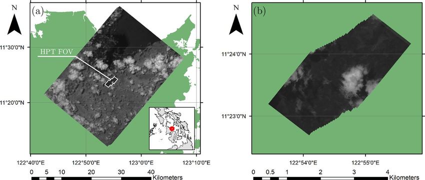
www.nature.com/scientificreports/                                                                   www.nature.com/scientificreports

                                                      HPT               SMI
                            Focal Length (mm)         974               48.2
                            Aperture (mm)             96                17.6
                            Exposure Time (ms)        2                 12
                            Ground Sampling Distance,
                                                      2.9               58.1
                            GSD (m) *
                                                      1.9 km × 1.4 km   38.3 km × 28.7 km
                            Field-of-View *
                                                      (0.29° × 0.22°)   (5.79° × 4.34°)

                           Table 1. Summary of the Specifications of SMI and HPT. The ground sampling distance and field-of-view were
                           estimated at nadir. * The value is estimated based on the altitudes as of image acquisition which is approximately
                           378.6 km at nadir and at a stationary state.

                           resolution of 15 or 90 m12,15, and reported time intervals of 2.5 to 7.5 min7,9,11,16,17. Furthermore, vertical accuracy
                           reported from past studies are typically 0.5 km7,9–12 to 1 km13,14. With the higher spatial resolution of DIWATA-1,
                           the vertical resolution of a cloud-top height measurement also increases due to the decrease in the error of the
                           disparity between stereoscopic images18. The shorter time interval between the image pairs further decreases the
                           error due to cloud advection and changing morphology.
                               Other cloud-top height measurement techniques such as using the cloud brightness temperature (or bispec-
                           tral method)—where the height (pressure) is determined by comparing the brightness temperature with vertical
                           sounding from a radiosonde or sounder19,20—have relatively low spatial resolution imagery15,21,22. However, the
                           vertical accuracy of this method can also reach 1.1 km20,23,24, depending on the emissivity of the clouds and accu-
                           racy of the vertical profile8,25. Using the atmospheric absorption bands of CO2 and O2 also results in a relatively
                           low spatial resolution25,26 and a reported vertical accuracy of 0.1 km to 1.5 km25,27,28. Furthermore, this technique
                           is based on the absorption difference, which varies slightly, of the cloud at two or more wavelengths29. LIDAR
                           and radar measurements are the sensors with the highest vertical resolution, as these can range from 7.5 m to 750
                           m30,31. However, these active sensors are technologically complex and expensive32,33.
                               The main goal of this study is to propose a methodology for and assess the capability and consistency of
                           the DIWATA-1 microsatellite to measure cloud-top heights by constructing three-dimensional models of clouds
                           through stereoscopy. The measured cloud-top heights are then compared with HIMAWARI-8’s 11.2 μm (Band-
                           14) and with cloud-edge heights obtained by measuring the distances from the clouds to their corresponding
                           shadows.

                           Instrument and Observations
                           Instrument. DIWATA-1 is a 50-kg microsatellite built by Filipino students in the Philippine Microsat (PHL-
                           MICROSAT) Program in collaboration with Hokkaido University and Tohoku University. It was launched into
                           an orbital altitude of 403 km from the Kibo module of the International Space Station (ISS) on April 27, 201634.
                           DIWATA-1 carries four optical payloads: a high-precision telescope (HPT) and wide-field camera, both of which
                           are similar to that aboard RISING-235; a space-borne multispectral imager (SMI); and a middle-field camera
                           (MFC). All images have a dimension of 659 by 494 pixels. However, unlike the HPT on RISING-235, the HPT of
                           DIWATA-1 does not include a liquid crystal tunable filter (LCTF); this is integrated in the SMI. In this study, the
                           SMI and the HPT were selected from among the four DIWATA-1 payloads for their advantageous spatial reso-
                           lutions. The SMI has a pixel resolution of 58.1 m and is a multi-spectral sensor with two charge-coupled devices
                           (CCDs) and captures a spectral image selectively in the visible (400–780 nm) and near-infrared (730–1020 nm)
                           regions at an interval of 1-nm. On the other hand, the HPT has a pixel resolution of 2.9 m and four CCDs that
                           capture images in the blue, green, red, and near-infrared regions. Table 1 shows the specifications of SMI and
                           HPT. With the exposure times given for the SMI and HPT, the actual sampling of the SMI increases from 58.1 m
                           to 94 m while that of the HPT increases to 16 m. One pixel of the SMI sensor can be contaminated by a neigh-
                           boring pixel, while an HPT pixel can be contaminated by as many as five pixels; this causes a blur in the images.
                               To avoid the saturation of measured radiances that occur in the visible band of SMI, the 870-nm band with
                           a full width at half maximum (FWHM) bandwidth of 10-nm was used. The HPT images were from the green
                           band, which is centered at 560 nm with ~45-nm FWHM bandwidth. Although two different bands were used in
                           this study, the reflectance of an optically thick or opaque cloud does not vary largely within the scopes of these
                           bands36–38.
                               The DIWATA-1 target-pointing capability was also utilized in this study; this allows the microsatellite to point
                           and lock the cameras to view a specific location as it moves through its orbit. Although stereoscopy-based meas-
                           urement of cloud-top heights can be performed with a camera in a steady position, as in the case of geosynchro-
                           nous satellites, DIWATA-1 traverses its orbit at an approximate speed of 7.6 km/s. Thus, it is necessary to use its
                           target-pointing capability so that the same scene and location are apparent in the captured images. DIWATA-1
                           rotates by an angle Δθ as it traverses its orbit. Thus,
                                                                         Δθ = θ ( t ) − θ ( t + Δt ) ,                                         (1)
                           where Δt is the time difference between two consecutive captures set to 200 ms. Theoretically, the angle θ (see
                           Fig. 1a) is subtended by the point directly below the satellite (i.e., the subsatellite point), and the central coordi-
                           nate of the image is given by the following equation:

Scientific Reports |   (2020) 10:7570 | https://doi.org/10.1038/s41598-020-64274-z                                                               2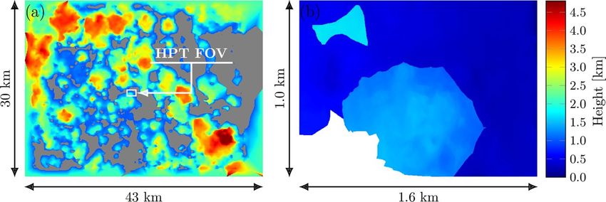
www.nature.com/scientificreports/ www.nature.com/scientificreports
Figure 1. (a) DIWATA-1, at 378.6-km altitude as on the day of capture, captured 30 images using both SMI and
HPT with a 200-ms time interval between captures. The angles θ(t ) and θ(t + Δt ) are those subtended by the
subsatellite point and the image centers at times t and t + Δt , respectively. The satellite rotated by ~0.23° with
every capture; this differs by 0.02° from the theoretical estimation for perfect target-pointing, and B is the
baseline, the distance traveled by DIWATA-1 after Δt . Also shown here is a point P, which is a point seen in
both Images 1 and 2. (b) Shows how the common point P is projected on Image 1, P1, and Image 2, P2, where Q(t )
and Q(t + Δt ) are the positions of the optical center of DIWATA-1 at time t and t + Δt , respectively, and e1 and
e2 are the epipoles of Images 1 and 2, respectively. The line passing through the projection of point P and the
epipole is called an epipolar line.
D( t ) − I ( t ) 180°
θ(t ) = arctan × ,
Z π (2)
where D(t ) is the along-track position of the subsatellite point at time t, I (t ) is the central coordinate of the image
captured at time t , Z is the satellite altitude relative to the subsatellite point, and θ(t ) is the view zenith angle at
time t . Note that this equation is valid only when the curvature of the Earth is negligible.
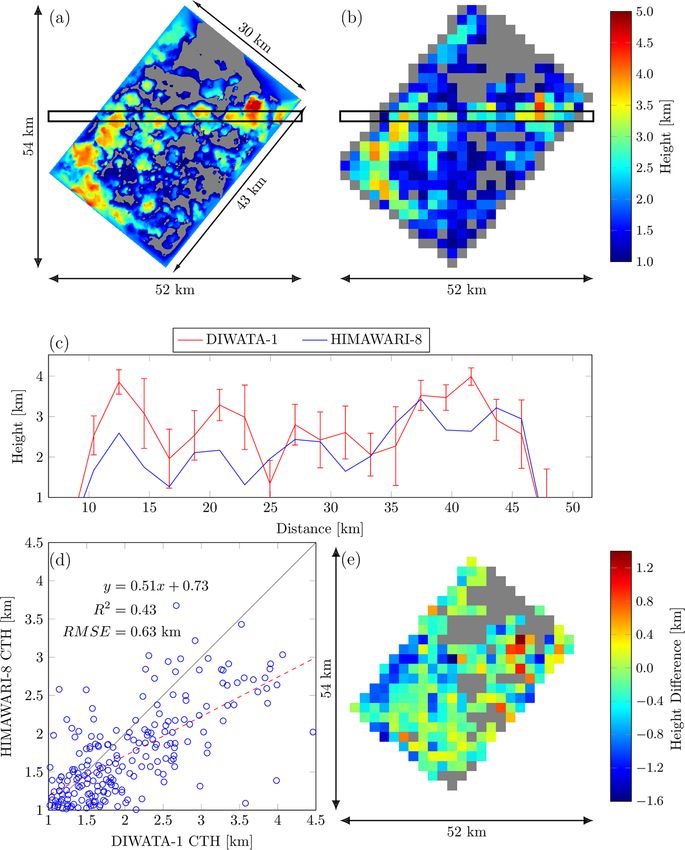
Observations. On August 5, 2017 DIWATA-1’s SMI and HPT successfully captured clouds hovering above
Iloilo province in the Philippines from 12:40:39 to 12:40:45 Philippine Standard Time (PST) or 04:40:39 to
04:40:45 Coordinated Universal Time (UTC). To minimize the cloud advection between each image, the interval
between each capture was set to the minimum possible value of 200 ms. In accordance with the total capture time,
each camera obtained a total of 30 images. Most clouds captured within the fields of view (FOVs) of the camera
seem to have been low-lying, and potentially stratocumulus or cumulus (Fig. 2). Since its release, the satellite’s
altitude has decreased to 378.6 km around the time the images were acquired for this study.
The images were then georeferenced, using surface features as control points, using ESRI ArcGIS 10.2.2, and
the coordinates of each pixel in the image were estimated. Figure 2 shows the georeferenced images captured by
the SMI and HPT via target-pointing. The HPT FOV is overlaid on the image captured by the SMI and is enclosed
with a white line. The center of the initial SMI image was located at approximately 11.41°N and 122.91°E. The final
image had a central position of 11.42°N and 122.93°E.
To find the rotation of the satellite due to target-pointing (see Eqs. 1 and 2), the two-line element dataset of
DIWATA-1 was entered into the orbital calculation software Systems Tool Kit (STK) 11.6 (developed by Analytical
Graphics, Inc.) to extract D and Z . For perfect target-pointing, that is I (t ) = I (t + Δt ) (see Fig. 1a), the average
value of Δθ between successive images is nominally 0.21°. However, as the target-pointing encounters an error at
a certain level, that is, I (t ) ≠ I (t + Δt ), the area captured by the telescope on the satellite shifts slightly from one
location to another. Using the central coordinates of the captured images while retaining the values for D and Z,
Δθ is, on average, ~0.23° from one location to another; this is a difference of 0.02° from the theoretical estimate.
Hence, the image centers are displaced by approximately 84 m, with the SMI and HPT image centers being dis-
placed by approximately 1.5 and 28 pixels, respectively. This displacement is not a significant problem as there are
overlaps exceeding 99% and 94% between consecutive SMI and HPT images, respectively.
Scientific Reports | (2020) 10:7570 | https://doi.org/10.1038/s41598-020-64274-z 3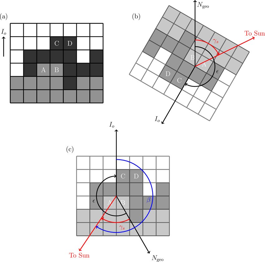
www.nature.com/scientificreports/                                                               www.nature.com/scientificreports

                           Figure 2. Images captured by (a) SMI and (b) HPT from 12:40:39 to 12:40:45 PST on 5 August 2017, stacked
                           from left to right. The HPT FOV is overlaid on (a), enclosed by a white line.

                           Figure 3. Analysis procedure for cloud-top height estimation from stereoscopic image set. The upper and lower
                           sections show the construction of the three-dimensional model from the images and estimation of the cloud-
                           top heights from the three-dimensional model, respectively.

                               On the same day as these images were taken, the Japanese weather satellite HIMAWARI-8 captured the
                           east-southeast Asian region at 12:40:00 PST, 39 seconds before DIWATA-1 captured the clouds above Iloilo.
                           HIMAWARI-8 has 16 spectral bands: 3 in the visible, 3 in the near-infrared, and 6 in the far-infrared region39.
                           The spatial resolution at the subsatellite points in the blue, green, and first near-infrared (0.86 μm) bands is 1 km;
                           for the red, it is 0.5 km, and for the other remaining bands the spatial resolution is 2 km. The cloud-top height
                           product on HIMAWARI-8 uses the brightness temperature measured by one of its far infrared bands, Band-14
                           (11.2-μm)21; this study compares that to DIWATA-1. Here, the brightness temperature is converted to cloud-top
                           height using a radiosonde measurement (see details in Appendix C).

                           Method
                           The three-dimensional model of the scene used to estimate the cloud-top height was generated from a set of ste-
                           reoscopic images in a Multi-view Stereo (MVS) algorithm-based40,41 software package RealityCapture 1.0.3.6310
                           RC, developed by Capturing Reality; this process is shown in Fig. 3 and is mainly composed of two work-
                           flows. First, a three-dimensional model of the scene was constructed from the stereoscopic images captured by
                           DIWATA-1 (upper portion of Fig. 3 workflow, enclosed by the solid rectangle); this was then used to estimate
                           cloud-top heights (bottom portion of Fig. 3 workflow, enclosed by the dashed rectangle).
                              In the “Image Alignment” block, the images were aligned based on their cloud and terrain surface features,
                           whose relative positions change in each image due to the movement of DIWATA-1. Assuming that the cloud
                           advection and the change in cloud morphology is negligible, the camera movement from one point to another
                           could be estimated from the differences of the feature positions; therefore, the camera position and/or orienta-
                           tion42, which is the “Relative Camera Position” output block in Fig. 3, could be determined. The next block, “3D
                           Model Construction”, constructs a three-dimensional model from the images by triangulating three-dimensional
                           points and estimating a potential surface patch from the features that lie within a set number of pixels from
                           the same epipolar line43 (see Fig. 1b). The maximum set of pixels was set to one, i.e., features that lie more than

Scientific Reports |   (2020) 10:7570 | https://doi.org/10.1038/s41598-020-64274-z                                                             4
www.nature.com/scientificreports/ www.nature.com/scientificreports
Figure 4. Three-dimensional models constructed from (a) SMI and (b) HPT images. The approximate HPT
FOV is overlaid on (a), enclosed in a white box. The axes on the lower-left indicate the model orientation.
one pixel from the same epipolar line are discarded by the software and are not used to create the model. These
patches then form a surfel (surface element) model43.
The camera focal length was also set to further assist the software with image alignment. In this process, as the
software requires 35-mm equivalent focal lengths f35mm as input, the camera focal lengths were converted accord-
ing to the following relationship44:
43.27mm
f35mm = × f,
S (3)
where 43.27 mm is the diagonal size of a film with 35-mm height, S is the diagonal size of the SMI/HPT sensor,
and f is the camera focal length. The diagonal size of the SMI and HPT sensors is 6.09 mm, and their focal lengths
are 48.2 and 974 mm, respectively. Using Eq. 3, the 35-mm equivalent focal lengths calculated are 0.342 m and
6.92 m for the SMI and HPT, respectively. Entering these values into the software will calibrate the estimated
camera positions of the software. However, this method was not applied to the HPT due to its large f35mm, rather
only the raw HPT images were used without additional inputs, and follows the workflow shown in Fig. 3. The
results of the three-dimensional model of the SMI, with the assistance of f35mm, and of the HPT, are shown in
Fig. 4a,b, respectively. The time it took for the software to align the images until to giving the model texture is
approximately 1.5 minutes for the SMI and 35 seconds for the HPT for a Windows 10 PC with Intel Core
i7–6700HQ CPU at 2.6 GHz, a RAM of 8.00 GB, and a graphics card of NVIDIA GTX950M. The software meas-
ures height and estimated camera positions in “units” by default; these are measured relative to the internal coor-
dinate system of the software as depicted by the gridded surface in Fig. 4. For the sake of discussion, these units
will be called “software units.” The models were made using 30 images for both SMI and HPT, and the estimated
camera altitudes of the software range from 420.3 to 420.8 software units and from 4,122.4 to 4,154.3 software
units for the SMI and HPT models, respectively. Compared to the raw images from DIWATA-1, the number of
pixels along the x- and y-directions increased to 1,113 by 800 pixels and 1,060 by 638 pixels for the SMI and HPT
models, respectively. Furthermore, because all DIWATA-1 images do not show what is below the clouds, the
three-dimensional models do not include cloud-base height data. Exporting the three-dimensional models from
the software results into raw digital elevation maps (DEMraw ) or surface elevation maps, where each point in the
map has a height, with respect from the gridded surface (expressed in software units), the clouds can be identified
as relatively high points on the DEM or through visual assessment. These estimated camera positions and the
heights of each pixel in the DEM are necessary to convert the measurements from software units into meters or
kilometers.
In the “Conversion Factor Calculation” block, a relationship between the estimated camera altitudes from the
software, expressed in software units, and the altitude of DIWATA-1, expressed in meters, at the time of acquisi-
tion. The conversion factor for the SMI and the HPT is given by the following:
h actual
κ= ,
h software (4)
where h actual is the altitude of DIWATA-1 generated by the STK software, expressed in meters, which differs by
around 1 km from the actual altitude of the microsatellite, while h software is the altitude of the camera as estimated
by RealityCapture, expressed in software units. However, because the camera positions estimated by the software
for the HPT were not calibrated using its f35mm focal length, the value of h software for the HPT were instead cali-
brated using the default 35-mm focal length output of the software, f ′35mm. The details of this process are pre-
sented in Appendix A. These results into a conversion factor κ of meters per software unit, which is then
multiplied to DEMraw to convert the measurements from software units to meters, i.e., DEMconv = κ ⋅ DEMraw ,
Scientific Reports | (2020) 10:7570 | https://doi.org/10.1038/s41598-020-64274-z 5www.nature.com/scientificreports/ www.nature.com/scientificreports
Figure 5. Cloud-top height results for (a) SMI and (b) HPT, converted from software units to meters. The
model sizes differ from the camera FOVs because the models are a combination of multiple images. Areas that
are colored gray are cloud-free regions.
where DEMconv is the DEM with height measurements taken in meters. The number of conversion factors κ in a
single DEM will be equal to the number of images used. In this study, the average of 30 conversion factors corre-
sponding to the 30 images were used for both the SMI and HPT.
The resulting cloud-top heights from the stereoscopic technique were compared to those of the cloud-shadow
technique and to the clouds’ brightness temperature. The purpose of this comparative analysis is to confirm
whether the cloud-top height measurements from the stereoscopic method are consistent with those derived
using other techniques. For the cloud-shadow technique, the height of a cloud-edge identified in the DEMconv was
compared to the corresponding cloud-edge whose height was estimated based on the shadow cast by the cloud
and solar angles. The details of this procedure are presented in Appendix B. On the other hand, the brightness
temperature approach uses the brightness temperature measured by HIMAWARI-8’s Band-14 (11.2-μm) and the
temperature vertical profile measured by a radiosonde to derive the cloud-top heights. The details of this proce-
dure are presented in Appendix C.
Results and Discussion
Cloud-top heights from stereoscopic technique. The images of clouds captured on August 5, 2017 at
12:40:39 to 12:40:45 PST were aligned to retrieve the estimated camera positions from RealityCapture. With the
STK-simulated positions and altitudes of DIWATA-1 at the capture time, the conversion factor κ (Eq. 4) was
estimated to measure the cloud-top heights in DEMconv . The average conversion factor for the SMI is
κ = 876.1 ± 2.3 m per software unit, while the HPT has κ = 89.2 ± 0.2 m per software unit. Figure 5a,b show
the digital elevation map DEMconv for the SMI and HPT, respectively. From Fig. 5a, the estimated cloud-top
heights range from 1.5 km to 4.5 km, which is indicative of low clouds and developed cumulus clouds and con-
firms the visual assessment carried out in Section 2.2. Figure 5b, however, shows a closer inspection of clouds with
heights ranging from 1.5 km to 2.0 km, which are also low. The masked region in Fig. 5b, covered in white, con-
tains erratic cloud-top height values due to the lack of overlapping features within this region, which is due to the
target-pointing error. The full image of the HPT is shown by Figure S1 in the supplementary material. From
DEMconv , the vertical resolutions were found to be 40 m and 2 m for the SMI and HPT, respectively.
With the baseline B, i.e. the distance traversed by the satellite between the first and last images, set at 45.6 km,
just as the focal lengths of the SMI and HPT and altitude of DIWATA-1 were (see Table 1), the theoretical error
Δh in the constructed DEM is as follows18,45:
H2
Δh = × Δp
fB (5)
where H is the altitude of DIWATA-1, f is the focal length, and Δp is set to 7.4 μm, which is the estimated dispar-
ity error for both SMI and HPT cameras. The resulting Δh ranges from 0.48 km to 0.49 km, and 0.024 km for the
SMI and HPT DEMs, respectively, accounting the simulation error of DIWATA-1’s altitude and if the cloud
advection and change in morphology is negligible. Otherwise, the disparity error may need to be adjusted, which
would result in errors of higher multiples of 0.48 km and 0.024 km or a complete failure of image alignment.
Another possible source of error for the DEMconv is the imperfect target-pointing (see Section 2.2), which is off by
0.02° from the theoretical estimate. Since DIWATA-1 was approximately 20 km away from the center of the target
at the final image capture, this could translate to an error of 1.1 km in the cloud-top height measurements46.
Comparison of the Stereoscopic-based Cloud-top Heights with that from other
Techniques. The cloud-top heights derived from the stereoscopic technique were compared to the
cloud-shadow-derived cloud-top heights. Measuring the cloud-edge heights through cloud-shadow technique
requires the solar angles (Appendix B). The solar zenith and azimuth angles throughout the duration of DIWATA-
1’s operation are, on average, 12.5° and 297.5°, respectively. Upon georeferencing, the images were rotated by
= 309° or −51° from their original orientation. From Eq. 11, the solar azimuth angle with respect to the original
orientation of the images β is approximately 348.5° or −11.5°. This value was used to pair cloud-edge pixels to
their corresponding shadow. Figure 6 shows a scatter plot of the estimated cloud-edge heights from the
Scientific Reports | (2020) 10:7570 | https://doi.org/10.1038/s41598-020-64274-z 6www.nature.com/scientificreports/ www.nature.com/scientificreports
Figure 6. Correlation between the Cloud-top Height results of Cloud-shadow and Stereoscopic Techniques in
the SMI. The solid gray line is the y = x line, which was overlaid for reference.
cloud-shadow technique and the cloud-edge heights estimated from DEMconv for the SMI. Multiple cloud-edge
points were gathered and correlated for the SMI. The cloud-shadow measurements correlate strongly with that of
DEMconv , with an R2 = 0.75 and a significance value p = 8.7 × 10⁻⁵, with a root-mean-square error (RMSE)
value of 0.35 km; most of the outliers are from thin and relatively small clouds. On the other hand, the average
difference between the stereoscopy-derived and the cloud-shadow-derived cloud-top heights for the HPT is ~30 m.
The cloud-top height from the DEMconv of SMI was also compared to HIMAWARI-8 Band-14 (11.2-μm)
brightness temperature data captured at 12:40:00 PST, 39 s before DIWATA-1 captured the same scene. Cloud-top
height estimation from the HIMAWARI-8 data was performed using brightness temperature conversion (see
details in Appendix C). The resulting cloud-top height from this technique is consistent with the HIMAWARI-8
cloud-top height standard product distributed by JAXA Himawari Monitor. The spatial resolution of the standard
product is ~5.0 km, which is ~100 times larger than the spatial resolution of SMI and 2.5 times larger than
HIMAWARI-8 Band-14, making most of the clouds seen by SMI unresolvable. By using a radiosonde measure-
ment, the cloud-top height can be derived at a higher spatial resolution.
Atmospheric vertical profiles observed by radiosondes flown over Cebu, 150 to 200 km from Iloilo, were used
in conjunction with the HIMAWARI-8 data. High-resolution radiosonde data, averaged over the period August
11–20, 2013, were employed47 to represent atmospheric conditions during the time that DIWATA-1 was acquiring
its images. Figure 7 shows a comparison of the cloud-top heights obtained from the DIWATA-1 SMI (Fig. 7a),
which was rotated to match the orientation of the HIMAWARI-8 data (Fig. 7b), as well as a cross-sectional
comparison of the two (Fig. 7c). The section being compared is bounded by the two horizontal black lines in
Fig. 7a,b. This cross-sectional region was chosen because majority of the pixels within this area are cloudy and
have non-zero cloud-top heights. The DIWATA-1 cloud-top height measurements shown in Fig. 7c were obtained
by averaging values within a region of 49 × 49 pixels of the rotated SMI model (Fig. 7a), which corresponds to a
single pixel of the HIMAWARI-8 data.
It is possible that the vertical temperature profile in Cebu may have differed from that at the SMI imaging
location. However, data from the Atmospheric Infrared Sounders (AIRS) satellite48 indicates that there is little
difference between the vertical profiles of Cebu and Iloilo; the maximum difference is ~0.8 K, which translates to
a height difference of less than 50 m.
Figure 7c clearly shows that the cloud-top heights estimated from the DIWATA-1 SMI DEMconv are greater
than that from the HIMAWARI-8 data, which is further verified by Fig. 7d,e. Figure 7d shows the correlation
between the cloud-top heights measured by HIMAWARI-8 and SMI, and Fig. 7e shows the differences in
HIMAWARI-8 and the upscaled DIWATA-1 cloud-top height measurements, where a negative difference indi-
cates a higher DIWATA-1 cloud-top height. The negative differences in the middle are due to the unresolved
clouds from HIMAWARI-8. The slope of the regression line in Fig. 7d between the two measurements is less than
one, which further indicates that DIWATA-1 measurements are generally higher than those from HIMAWARI-8,
with both measurements having an R2 of 0.43 and an RMSE of 0.63 km. Overall, the absolute difference in
cloud-top heights has an average of 0.15 km with a standard deviation of 0.30 km. One of the possible sources of
this difference is the conversion of the HIMAWARI-8 brightness temperature to cloud-top heights, which was
only achieved by converting the former to the latter directly using an atmospheric vertical profile. This method
can be improved by further analyzing the consistency between the brightness temperature measured by satellites
and that of radiosondes, which could be a subject of future studies. However, it has been reported that the
cloud-top height product of HIMAWARI-8 can be under-estimated compared to the results from the Moderate
Resolution Imaging Spectroradiometer (MODIS) and the Cloud-Aerosol LIDAR and Infrared Pathfinder Satellite
Observations (CALIPSO)49. Another possible explanation is the low spatial resolution of the HIMAWARI-8
Band-14, which is ~2.0 km, compared with that of the DIWATA-1 SMI, which is 58.1 m7.
Scientific Reports | (2020) 10:7570 | https://doi.org/10.1038/s41598-020-64274-z 7www.nature.com/scientificreports/ www.nature.com/scientificreports
Figure 7. Comparison of (a) DIWATA-1 SMI and (b) HIMAWARI-8 cloud-top height results, where the gray
areas are relatively cloud-free pixels. (c) Cross-section of cloud-top heights in (a) and (b) for region between
black horizontal lines (Himawari 8/9 gridded data are distributed by the Center for Environmental Remote
Sensing (CEReS), Chiba University, Japan); (d) correlation between HIMAWARI-8 and SMI, where the solid
gray line is the y = x line, which was overlaid for reference; and (e) Cloud-top height difference between the
upscaled SMI and HIMAWARI-8.
Conclusions
Using data from DIWATA-1, this study constructed three-dimensional cloud models (DEMs) at higher spatial
and temporal resolutions than those previously reported7,9,11,13,15–17,21,22,25,26. Cloud-top heights were measurable
for 6-second observations with a 200-ms interval between captures, with 40-m and 2-m vertical resolutions for
SMI and HPT, respectively. The estimated RMSE with the cloud-edge height determined using the cloud-shadow
technique for the SMI is 0.35 km and has a correlation coefficient of 0.75 when compared with DIWATA-1. The
maximum difference of 30 m between the cloud-shadow derived and stereoscopy-derived cloud-top heights on
the HPT might have been due to the lack of variation in the sample points from the cloud-shadow cloud-edge
height measurements. An average difference of 0.15 km, with a maximum difference of 1.7 km relative to a rough
estimation from the HIMAWARI-8 Band-14 data was also obtained. Comparison with other cloud-top measur-
ing satellites such as MODIS, CALIPSO, MISR, LIDARs, and others that can measure cloud-top heights can be
done to further assess the technique presented in this study.
This study developed a novel and cost-effective approach to direct cloud-top height estimation using a micro-
satellite. By optimizing the minimum images required to construct a DEM, several subsets of images may be
Scientific Reports | (2020) 10:7570 | https://doi.org/10.1038/s41598-020-64274-z 8www.nature.com/scientificreports/ www.nature.com/scientificreports
extracted from a single set captured from a single pass of the microsatellite. These subsets may then construct
multiple DEMs and reflect the cloud-top height from the time interval between each subset; this will then meas-
ure the vertical development of the clouds. However, the baseline will become shorter for each DEM, increasing
the possible error in the cloud-top height measurement; therefore, it is desirable to have a constellation of micro-
satellites with capabilities similar to DIWATA-1 as this will decrease the error due to the short baseline. This has
been the practice to date, with two or more geostationary satellites for measuring cloud-top heights stereoscopi-
cally. The ability to obtain high spatial and temporal resolutions of cloud-top height is crucial for monitoring the
development of thunderstorms and understanding severe weather phenomena50.
Appendix A: Calibration of Camera Altitudes for the HPT. First, the optical system of the HPT was
assumed to obey the thin-lens approximation, where the distance between the object and the lens is interpreted
as the altitude of DIWATA-1. To utilize the altitude of DIWATA-1 as a basis for converting software units to abso-
lute units, like that of the SMI model, the distance between the cameras and the internal coordinate system of the
software should be known. However, as the focal length outputs of the software are expressed in 35-mm equiva-
lent focal lengths, the indication is that the distance between the camera and the internal coordinate system of the
software is based on f35mm. To resolve this, the focal length outputs of the software f ′35mm were converted to
actual focal lengths using the inverse of Eq. 3,
f ′35mm
f′ = × S,
43.27 mm (6)
′
where f ′ is the equivalent focal lengths of f 35mm. By knowing the relationship between the focal length of the HPT
and f ′ the distance between the cameras and the model in the software based on f ′ can be determined. The rela-
tionship between fHPT and f ′ is defined to be
f′
n= ,
fHPT
f′
=
974 mm (7)
Therefore,
1 1 1
= + ,
fHPT do ,HPT d i ,HPT
1 1 1
= + ,
n ⋅ fHPT n ⋅ do ,HPT n ⋅ d i ,HPT
1 1 1
= +
f′ do di (8)
where do,HPT is the altitude of DIWATA-1, d i,HPT is the distance between the HPT lens and image sensor, while do
and d i are the distances of the object and image, respectively, in relation to f ′. By multiplying n to the altitude of
DIWATA-1, the altitude of the cameras relative to f ′ can be determined. The input for h software for Eq. 4 will then
be n , or simply h actual is do.
h software
Appendix B: Cloud Identification and Height Estimation using the Cloud-Shadow tech-
nique. The values of the cloud-top heights from DEMconv were compared to a cloud-top height derived using
the cloud-shadow technique, which requires the solar zenith, azimuth angles and distance between the cloud-edge
and the edge of its shadow.
Figure 8a illustrates a cloud and shadow image (pixels are shown as boxes in a grid), where gray-filled boxes
are cloud pixels and black-filled boxes are shadow pixels corresponding to the cloud pixels. The first stage to
properly match a cloud edge to its shadow, i.e., to know whether the pixel labeled “A” matches with pixel “C” or
“D”, uses the solar azimuth angle.
The solar zenith αs and azimuth angles γs were estimated by the following51,52:
sin(αs ) = cos(δ )cos(φ)cos(ω) + sin(δ )sin(φ) (9)
sin(δ )cos(φ) − cos(δ )sin(φ) cos(ω)
cos(γs ) =
cos(αs ) (10)
where δ is the solar declination, φ is the latitude coordinate of the target, and ω is the hour angle, where all three
parameters are expressed in degrees.
The direction of the cloud shadow should be 180° away from the solar azimuth angle, which is relative to the
geographic north. To know the orientation of the geographic north Ngeo relative to the original orientation of the
image Io, the image should first be georeferenced (Fig. 8b). Where the angle between Ngeo and Io (the angle how
much the image has rotated) is indicated by ε (Fig. 8c) given the convention that clockwise or north-to-east rota-
tion is positive. The solar azimuth angle relative to Io, β , can be estimated as follows:
Scientific Reports | (2020) 10:7570 | https://doi.org/10.1038/s41598-020-64274-z 9www.nature.com/scientificreports/ www.nature.com/scientificreports
Figure 8. (a) Sample set of image pixels with the gray-filled squares as clouds and black-filled squares as their
corresponding shadow; (b) Orientation of the image after georeferencing where γs is the solar azimuth angle
relative to the geographic north and ε as the angle between the geographic north and the original orientation
of the image; and (c) is the original orientation of the image overlaid with the direction of the geographic
north and solar azimuth angle from the geographic north. The angle β is the solar azimuth angle relative to the
original orientation of the image.
β = 360° − + γs . (11)
Therefore,
Ax − Cx
tan(β ) =
Ay − Cy (12)
where Ax and Cx are the x-coordinates of pixel “A” and “C”, respectively, and Ay and Cy are the y-coordinates of the
same pixels, respectively. At times when the shadow pixel is difficult to identify due to the spatial resolution of the
camera, the horizontal and vertical pixel distance combination with the value nearest to tan(β ) will be chosen. In
cases where β = 90° or 270°, the shadow pixel is directly left or right of the cloud pixel, respectively, and if β = 0°
or 180°, the shadow pixel is directly below or above the cloud pixel, respectively.
Using β and the original orientation of the image to count the horizontal and vertical pixel distances between
a cloud and a shadow removes the possible changes in the ground sampling distance (GSD) of the image caused
by the rotation of the georeferencing. However, because there are cases in which the cloud and/or the cloud
shadow pixel contaminates their surrounding pixels, it is possible that the cloud or cloud shadow is actually
located at the neighbors of the chosen pixel. To account for this uncertainty, the height error of a cloud-edge esti-
mated from this technique corresponds to a single pixel.
After identifying the shadow pixel, the distance dcs between the cloud and shadow pixel is estimated by the
Euclidean distance multiplied by the GSD of the image as below,
2
dcs = GSD × (
(Ax − Cx )2 + Ay − Cy ) (13)
The height of the cloud edge pixel hc is then estimated via,
hc = dcs tan(90° − αs ) . (14)
Appendix C: Conversion of the Brightness Temperature of HIMAWARI-8 to Cloud-top
Heights. The cloud-top heights measured using the DIWATA-1 stereoscopic technique was compared with
those obtained using HIMAWARI-8. To properly compare the two, the brightness temperature measured by
HIMAWARI-8 was converted to cloud-top height using a radiosonde sounding.
The radiosonde used is the Vaisala RS41, which measures the temperature profile of the atmosphere as a func-
tion of altitude (the uncertainty of the instrument for measuring altitude is 10 m while for temperature it is
0.3 °C53), T (z ) where z is the altitude of the radiosonde, expressed in meters from sea level, and T is the tempera-
ture expressed in degrees Celsius at altitude z . The temperature profile was measured every 2 s in the raw data and
converted to a range from 25 m to 16,500 m—the temperature of the atmosphere at this range is inversely propor-
tional with altitude—with a step size of 25 m.
Scientific Reports | (2020) 10:7570 | https://doi.org/10.1038/s41598-020-64274-z 10www.nature.com/scientificreports/ www.nature.com/scientificreports
Given a brightness temperature BT measured by HIMAWARI-8’s Band-14 (11.2-μm), there is an interval
T (z i ) ≥ BT > T (z i +1), where z i < z i +1
where i is the i-th data point in the radiosonde data. Under the assumption that the change in temperature
between z i and z i +1 is linear, the corresponding altitude of BT , zBT , can be found through linear interpolation.
z i+1 − z i
zBT = [BT − T (z i )]
T (z i +1) − T (z i )
However, cloud-top height errors arising from this technique lie in the similarity between the
radiosonde-measured cloud-top temperature and satellite-measured cloud-top brightness temperature.
Differences can range from less than 2.5 °C to 30 °C for warm clouds54, which is the case in this study, and
cloud-top height measurements can differ typically by 1.5 km55.
To collocate DEMconv from SMI with HIMAWARI-8’s Band-14 (11.2-μm), it was upscaled to match the 2-km
spatial resolution of HIMAWARI-8 after orienting it at the same orientation as the HIMAWARI-8 data.
Received: 28 June 2019; Accepted: 14 April 2020;
Published: xx xx xxxx
References
1. Snodgrass, E. R., Di Girolamo, L. & Rauber, R. M. Precipitation characteristics of trade wind clouds during RICO derived from
radar, satellite, and aircraft measurements. J. Appl. Meteorol. Climatol. 48, 464–483 (2009).
2. Adler, R. F. & Mack, R. A. Thunderstorm cloud height-rainfall rate relations for use with satellite rainfall estimation techniques. J.
Climate Appl. Meteor. 23, 280–296 (1984).
3. Biondi, R., Ho, S.-P., Randel, W., Syndergaard, S. & Neubert, T. Tropical cyclone cloud-top height and vertical temperature structure
detection using GPS radio occultation measurements. J. Geophys. Res. Atmos. 118, 5247–5259 (2012).
4. Jensen, E. et al. Formation of a tropopause cirrus layer observed over Florida during CRYSTAL-FACE. J. Geophys. Res. Atmos. 110,
1–17 (2005).
5. Wong, V. & Emanuel, K. Use of cloud radars and radiometers for tropical cyclone intensity estimation. Geophys. Res. Lett. 34, 16–19
(2007).
6. Luo, Z. et al. On the use of CloudSat and MODIS data for estimating hurricane intensity. Geosci. Remote Sense. Lett. 5, 13–16 (2008).
7. Mack, R., Hasler, A. F. & Rodgers, E. B. Stereoscopic observations of hurricanes and tornadic thunderstorms from geosynchronous
satellites. Adv. Space Res. 2, 143–151 (1983).
8. Simpson, J., McIntire, T., Jin, Z. & Stitt, J. R. Improved cloud top height retrieval under arbitrary viewing and illumination conditions
using AVHRR data. J. Remote Sens. Environ. 72, 95–110 (2000).
9. Seiz, G., Tjemkes, S. & Watts, P. Multiview cloud-top height and wind retrieval with photogrammetric methods: application to
METEOSAT-8 HRV observations. J. Appl. Meteorol. Climatol. 46, 1182–1195 (2007).
10. Takashima, T., Takayama, Y., Matsuura, K. & Naito, K. Cloud height determination by satellite stereoscopy. Pap. Meteor. Geophys. 33,
65–78 (1982).
11. Moroney, C., Davies, R. & Muller, J. P. Operational retrieval of cloud-top heights using MISR data. IEEE Trans. Geosci. Remote Sens.
40, 1532–1540 (2002).
12. Seiz, G., Davies, R. & Grün, A. Stereo cloud-top height retrieval with ASTER and MISR. Int. J. Remote Sens. 27, 1839–1853 (2006).
13. Prata, A. J. & Turner, P. J. Cloud-top height determination using ATSR data. Remote Sens. Environ. 59, 1–13 (1997).
14. Naud, C. et al. Comparison between ATSR-2 stereo, MOS O2-A band and ground-based cloud top heights. Int. J. Remote Sens. 28,
1969–1987 (2007).
15. Genkova, I., Seiz, G., Zuidema, P., Zhao, G. & Di Girolamo, L. Cloud top height comparisons from ASTER, MISR, and MODIS for
trade wind cumuli. J. Remote Sens. Environ. 107, 211–222 (2007).
16. Hirano, A., Welch, R. & Lang, H. Mapping from ASTER image data: DEM validation and accuracy assessment. ISPRS J. Photogramm.
Remote Sens. 57, 356–370 (2003).
17. Mutlow, C., Murray, J., Bailey, P., Birks, A. & Smith, D. ATSR-1/2 User Guide (1999).
18. Haggrén, H. Stereoscopy application of spherical imaging. Proc. SPIE. 5665, 89–95 (2005).
19. Shenk, W. E. & Curran, R. J. A multi-spectral method for estimating cirrus cloud top heights. J. Appl. Meteor. 12, 1213–1216 (1973).
20. Reynolds, D. W. & Vonder Haar, T. H. A bispectral method for cloud parameter determination. Mon. Weather Rev. 105, 446–457
(1977).
21. Mouri, K., Hiroshi, S., Yoshida, R. & Izumi, T. Algorithm theoretical basis document for cloud top height product. Meteorological
Satellite Center Technical Note 61, 33–42, https://www.data.jma.go.jp/mscweb/technotes/msctechrep61-3.pdf (2016).
22. Di Michele, S., McNally, T., Bauer, P. & Genkova, I. Quality assessment of cloud-top height estimates from satellite IR radiances
using the CALIPSO lidar. IEEE Geosci. Remote Sens. 51, 2454–2464 (2013).
23. Randriamampianina, R., Nagy, J., Balogh, T. & Kerényi, J. Determination of cloud top height using meteorological satellite and radar
data. Phys. Chem. Earth (B). 25, 1103–1106 (2000).
24. Naud, C. M., Muller, J.-P., Clothiaux, E. E., Baum, B. A. & Menzel, W. P. Intercomparison of multiple years of MODIS, MISR, and
radar cloud-top heights. Ann. Geophys. 23, 2415–2424 (2005).
25. Menzel, W. P., Smith, W. L. & Stewart, T. R. Improved cloud motion wind vector and altitude assignment using VAS. J. Climate Appl.
Meteor. 22, 377–384 (1983).
26. Platnick, S. et al. The MODIS cloud products: algorithms and examples from. Terra. IEEE Trans. Geosci. Remote Sens. 41, 459–473
(2003).
27. Frey, R. A. et al. A comparison of cloud top heights computed from airborne lidar and MAS radiance data using CO2 slicing. J.
Geophys. Res. 104, 24547–24555 (1999).
28. Preusker, R., Fischer, J., Albert, P., Bennartz, R. & Schüller, L. Cloud-top pressure retrieval using the oxygen A-band in the IRS-3
MOS instrument. Int. J. Remote Sens. 28, 1957–1967 (2007).
29. Fischer, J. & Grassl, H. Detection of cloud-top height from backscattered radiances within the oxygen A-band part I: theoretical
study. J. Appl. Meteor. 30, 1245–1259 (1991).
30. Marais, W. J. et al. Approach to simultaneously denoise and invert backscatter and extinction from photon-limited atmospheric lidar
observations. Appl. Optics 55, 8316–8334 (2016).
31. Kim, S.-W., Chung, E.-S., Yoon, S.-C., Sohn, B.-J. & Sugimoto, N. Intercomparisons of cloud-top and cloud-base heights from
ground-based Lidar, CloudSat and CALIPSO measurements. Int. J. Remote Sens. 32, 1179–1197 (2011).
Scientific Reports | (2020) 10:7570 | https://doi.org/10.1038/s41598-020-64274-z 11www.nature.com/scientificreports/ www.nature.com/scientificreports
32. El Hajj, M. et al. Interest of integrating spaceborne LiDAR data to improve the estimation of biomass in high biomass forested areas.
Remote Sens. 9, 1–19 (2017).
33. Kiemle, C. et al. Potential of spaceborne lidar measurements of carbon dioxide and methane emissions from strong point sources.
Remote Sens. 9, 1–16 (2017).
34. Japan Aerospace Exploration Agency, The Philippines’ 50-kg-class microsatellite “DIWATA-1” has been received. DIWATA-1 will
be released from Kibo this spring iss.jaxa.jp/en/kiboexp/news/160203_diwata1_sat.html (2016).
35. Sakamoto, Y. et al. Development and flight results of microsatellite bus system for RISING-2. Trans. JSASS Aerospace Tech. Japan. 14,
89–96 (2016).
36. Xu, M., Pickering, M., Plaza, A. J. & Jia, X. Thin cloud removal based on signal transmission principles and spectral mixture analysis.
IEEE Trans. Geosci. Remote Sens. 54, 1659–1669 (2016).
37. Gao, B.-C., Han, W., Tsay, S. C. & Larsen, N. F. Cloud detection over the Arctic region using airborne imaging spectrometer data
during the daytime. J. Appl. Meteor. 37, 1421–1429 (1998).
38. National Operational Hydrologic Remote Sensing Center. 1.6 m Wavelength Important for Operational Remote Sensing at NOAA,
https://www.nohrsc.noaa.gov/technology/avhrr3a/avhrr3a.html (2011).
39. Japan Meteorological Agency. Imager (AHI), https://www.data.jma.go.jp/mscweb/en/himawari89/space_segment/spsg_ahi.html
(2013).
40. Gabara, G. & Sawicki, P. Accuracy study of close range 3D object reconstruction based on point clouds. BGC Geomatics. 25—29
(2017).
41. Jancosek, M., Shekhovtsov, A. & Pajdla, T. Scalable multi-view stereo. ICCV Workshop. 1526—1523 (2009).
42. Grussenmeyer, P. & Al Khalil, O. Solutions for exterior orientation in photogrammetry: a review. Photogramm. Rec. 17, 615–634
(2002).
43. Furukawa, Y. & Ponce, J. Accurate, dense, and robust multi-view stereopsis. IEEE T. Pattern Anal. 32, 1362–1376 (2009).
44. Standardization Committee. Guideline for noting digital camera specifications in catalogs. CIPA DCG-001-Translations-2005. at,
http://www.cipa.jp/std/documents/e/DCG-001_E.pdf
45. Eiken, T. & Sund, M. Photogrammetric methods applied to Svalbard glaciers: accuracies and challenges. Polar Res. 31, 1–16 (2012).
46. Zhao, W. & Nandhakumar, N. Effects of camera alignment errors on stereoscopic depth estimates. Pattern Recognit. 29, 2115–2126
(1996).
47. Kubota, H., Shirooka, R., Matsumoto, J., Cayanan, E. O. & Hilario, F. D. Tropical cyclone influence on the long-term variability of
Philippine summer monsoon onset. Prog. Earth. Planet. Sci. 4, 27, https://doi.org/10.1186/s40645-017-0138-5 (2017).
48. National Aeronautics and Space Administration. AIRS: The Atmospheric Infrared Sounder on NASA’s Aqua Satellite https://web.
archive.org/web/20130218142301/http://airs.jpl.nasa.gov/documents/factsheets_posters/AIRS-Data-Products-Brochure.pdf
(2013).
49. Mouri, K., Izumi, T., Suzue, H. & Yoshida, R. Algorithm theoretical basis for cloud type/phase product. Meteorological Satellite
Center Technical Note 61, 19–31, https://www.data.jma.go.jp/mscweb/technotes/msctechrep61-2.pdf (2016).
50. Mecikalski, J. R., Jewett, C. P., Apke, J. M. & Carey, L. D. Analysis of cumulus cloud updrafts as observed with 1-min resolution super
rapid scan GOES imagery. Mon. Weather Rev. 144, 811–830 (2016).
51. Vermote, E. et al. Second Simulation of a Satellite Signal in the Solar Spectrum – Vector (6SV), http://6s.ltdri.org/pages/manual.html
(2006).
52. Sproul, A. Derivation of the solar geometric relationships using vector analysis. Renew. Energy 32, 1187–1205 (2007).
53. Vaisala. Vaisala Radiosonde RS41-SG. B211321EN-J. at, https://www.vaisala.com/sites/default/files/documents/RS41-SG-
Datasheet-B211321EN.pdf
54. Landolt, S. D., Bateman, R. E. & Bernstein, B. C. A comparison of satellite and sounding derived cloud top temperature. Preprint at,
https://ams.confex.com/ams/pdfpapers/72249.pdf (2004).
55. Holland, L. et al. A comparison of the cloud top height product (CTOP) and cloud-top heights derived from satellite, rawinsonde,
and radar. Preprint at, https://ams.confex.com/ams/pdfpapers/105374.pdf (2006).
Acknowledgements
The PHL-Microsat Program, a Philippine Government program, is jointly undertaken by the University of the
Philippines Diliman, Hokkaido University, Tohoku University, the Advanced Science and Technology Institute
(ASTI), and the Philippine Council for Industry, Energy, and Emerging Technology Research and Development
(PCIEERD) of the Department of Science and Technology (DOST).The present work was supported by the Japan
Science and Technology Agency (JST) and Japan International Cooperation Agency (JICA) and JST under the
Science and Technology Research Partnership for Sustainable Development (SATREPS) and the Understanding
Lightning And Thunderstorms For Extreme Weather Monitoring And Information Sharing (ULAT) project
funded by the Philippines Department of Science and Technology (DOST). The DIWATA-1 data was provided
by the PHL-Microsat Program. The authors would also like to sincerely acknowledge and thank the reviewers for
their hard work and patience on reviewing this manuscript, and whose suggestions and comments have helped us
to improve and clarify it; we have learned along the way.
Author contributions
Ellison Castro developed the methods and did the analysis of the models, under the supervision of Tetsuro Ishida,
Yukihiro Takahashi and guidance of Gay Jane Perez and Joel S. Marciano, Jr; Hisayuki Kubota provided the
atmospheric vertical profile for the conversion of HIMAWARI-8 data to cloud-top heights. All authors revised
and reviewed the manuscript.
Competing interests
The authors declare no competing interests.
Additional information
Supplementary information is available for this paper at https://doi.org/10.1038/s41598-020-64274-z.
Correspondence and requests for materials should be addressed to E.C. or T.I.
Reprints and permissions information is available at www.nature.com/reprints.
Publisher’s note Springer Nature remains neutral with regard to jurisdictional claims in published maps and
institutional affiliations.
Scientific Reports | (2020) 10:7570 | https://doi.org/10.1038/s41598-020-64274-z 12www.nature.com/scientificreports/ www.nature.com/scientificreports
Open Access This article is licensed under a Creative Commons Attribution 4.0 International
License, which permits use, sharing, adaptation, distribution and reproduction in any medium or
format, as long as you give appropriate credit to the original author(s) and the source, provide a link to the Cre-
ative Commons license, and indicate if changes were made. The images or other third party material in this
article are included in the article’s Creative Commons license, unless indicated otherwise in a credit line to the
material. If material is not included in the article’s Creative Commons license and your intended use is not per-
mitted by statutory regulation or exceeds the permitted use, you will need to obtain permission directly from the
copyright holder. To view a copy of this license, visit http://creativecommons.org/licenses/by/4.0/.
© The Author(s) 2020
Scientific Reports | (2020) 10:7570 | https://doi.org/10.1038/s41598-020-64274-z 13You can also read