Digital Data Transmission
←
→
Page content transcription
If your browser does not render page correctly, please read the page content below
Module: Digital Communications

            Experiment 702

Digital Data Transmission

    Institut für Nachrichtentechnik E-8
 Technische Universität Hamburg-Harburg
ii
Table of Contents

Introduction ................................................................................................................................................... 1
Digital Transmission System ........................................................................................................................ 2
1 Digital Modulation Methods .................................................................................................................... 3
   1.1 Linear Modulation in the Baseband .................................................................................................. 3
       1.1.1 Quadrature Modulator QM ........................................................................................................ 6
       1.1.2 Quadrature Demodulator QDM ................................................................................................. 7
   1.2 Preparatory Problems ........................................................................................................................ 8
2 The Transmission channel ..................................................................................................................... 10
   2.1 Frequency Selective Time-Invariant Wireless Channel .................................................................. 10
   2.2 Channel Estimation Methods .......................................................................................................... 10
   2.3 Preparatory Problems ...................................................................................................................... 11
3 Equalization ........................................................................................................................................... 13
   3.1 Zero-Forcing Equalization .............................................................................................................. 14
   3.2 Minimum Mean Square Error Equalization .................................................................................... 14
   3.3 Baseband vs. Bandpass Signal ........................................................................................................ 15
   3.4 Preparatory Problems ...................................................................................................................... 16
4 Design of the Experiment ...................................................................................................................... 17
   4.1 Model .............................................................................................................................................. 17
   4.2 Experiment ...................................................................................................................................... 18
       4.2.1 Evaluation of Various Modulations ......................................................................................... 18
       4.2.2 Channel Measurement.............................................................................................................. 19
       4.2.3 Signal Equalization .................................................................................................................. 20
Bibliography ............................................................................................................................................... 22

                                                                                                                                                         iii
Introduction This practical course deals with the characteristics of digital data transmission. The technical task consists in transmitting binary data from a data source (e.g. a terminal) to a spatially distant data sink (e.g. a computer). It is necessary for digital voice and image transmission to carry out the sampling and quantization of analog source signals, since the majority of data and measurements exist in digital form. Realistic transmission channels have characteristic properties, whereby error-free reception of the transmitted data symbols is frequently prevented. Typical error-causing influences include additive noise interference, impulse disturbances, multipath propagation, frequency drift, and linear and non-linear distortion. In this practical course we will consider carrier- modulation methods and focus on the treatment of linear distortion of transmitted data signals. This task leads to the problem of signal equalization, for which classical solution methods exist. For the execution of this practical course a suitable technical model will be used. Transmitter and receiver filters as well as the transmission channel are digitally implemented. A modern signal processor thereby serves as a basis for the realization of the provided task. A more thorough look at the theoretical context is provided by the lecture “Mobile Communications” at the Hamburg University of Technology, as well as a number of textbooks [Pro08] [Skl01] [Lük07] [Boc83]. 1
Digital Transmission System

The complete transmission system that will be considered in this practical course can be seen
in the picture above. Initially, the fundamentals of the individual components “transmitter,”
“channel,” and “receiver” will be defined in order to lay the groundwork for the practical part
of this course. The digital modulation takes place on the transmitting end and is expressed by
the block [symbol mapping]. The block [ ( )] characterizes a pulse shaping filter which
creates a time-continuous baseband signal. Before a signal can be transmitted over the
[channel] the baseband signal must be transformed into a bandpass signal, which is carried
out by the quadrature modulator [QM]. The transmit signal is superimposed with a noise
signal ( ). On the receiving end the received signal ( ) is transformed back into a
baseband signal by the quadrature demodulator [QDM]. A “matched filter” [ ( )] increases
the signal-to-noise ratio of the received signal. An equalizer [EQ] is used to remove
intersymbol interferences (ISI) in the received signal.

                                                                                             2
1 Digital Modulation Methods
In comparison to analog modulation methods (amplitude, phase or frequency modulation),
digital modulation methods are more sensitive with respect to disturbances. Through suitable
choice of discrete value modulation symbols, represented in a so-called constellation
diagram, disturbances caused by noise influences in the received signal can be identified and
eliminated. Through these digital techniques transmission methods can be designed which
achieve very high bandwidth efficiency. Channel coding methods allow for additional
possibilities such as automatic bit error correction.
After an analog speech signal has been sampled and quantized, the resulting bit sequence can
be transmitted by a digital modulation method. The transmitted signal can thereby be
optimally suited to the channel characteristics through selection of the transmission and
modulation methods. By mapping the binary transmissions to the discrete modulation
symbols represented in the constellation diagram, each ( ) bit of a bit sequence to
be transmitted is bijectively assigned to one of a total of possible modulation symbols .
Each chosen modulation symbol is respectively multiplied with the so-called modulation
impulse ( ) of the period in the baseband.
1.1 Linear Modulation in the Baseband
Figure 1.1 Modulation in the baseband
Figure 1.1 illustrates the principle of digital modulation in a block diagram. The symbol
mapping determines which type of digital modulation will be used. The bit sequence to be
transmitted is initially subdivided into blocks of bits. Each of these blocks is uniquely
assigned to one of the possible complex-valued modulation symbols .A
modulation impulse ( ) is multiplied with the real and imaginary parts of the modulation
symbol, whereby two analog baseband signals exist, as can be seen by the following
equations. The form of the modulation impulse ( ) has a significant influence on the
spectral characteristics of the transmission signal.
31.1 Linear Modulation in the Baseband
( ) ∑ ( ) (1.1)
( ) ∑ ( ) (1.2)
( ) ( ) ( ) (1.3)
Figure 1.2 illustrates the constellation diagram of a quadrature phase-shift keying (QPSK)
with the four characteristic modulation symbols. Additionally, the complex-valued baseband
signal is plotted on the time axis separately for real and imaginary parts. The modulation
symbol can be directly identified by the phase state of the time signal.
Figure 1.2 Modulation example
41 Digital Modulation Methods
Further digital modulation methods are amplitude-shift keying (ASK) and quadrature
amplitude modulation (QAM). The respective modulation symbols are illustrated in Figure
1.3.
Figure 1.3 Modulation symbols
51.1 Linear Modulation in the Baseband
1.1.1 Quadrature Modulator (QM)
Figure 1.4 Transmitter-end quadrature modulation
For carrier modulation methods the high frequency and real-valued bandpass signal is created
in the quadrature modulator, whereby real and imaginary parts of the complex-valued
baseband signal ( ) are multiplied with √ ( ), respectively with
√ ( ).
Since cosine and sine signals are orthogonal to each other, the respective parts of the real-
valued bandpass signal can be separated from each other again in the receiver. The phase
relationship between cosine and sine is expressed mathematically with the aid of complex
numbers. The real-valued bandpass signal ( ) is calculated as follows:
( ) √ { ( ) } (1.4)
This representation is independent of the chosen modulation method and allows for the
technical realization of the high-frequency bandpass signal in the baseband.
61 Digital Modulation Methods
1.1.2 Quadrature Demodulator (QDM)
Figure1.5 Receiver-end quadrature demodulation
The quadrature demodulator is the counterpart of the quadrature modulator and is located in
the receiver. Its task is to transform the received high-frequency bandpass signal ( ) back
into a baseband signal ( ). The received real-valued bandpass signal ( ) is mixed into
the baseband through multiplication with the function √ ( ), respectively with
√ ( ). The mixed products that arise from the mixing process with doubled carrier
frequency are eliminated with a suitable low pass filter. This circumstance is illustrated in
Figure 1.5.
71.2 Preparatory Problems
1.2 Preparatory Problems
Problem 1
What are the advantages of digital modulation methods compared to analog ones?
Problem 2
For an 8-PSK modulation the following bit phase assignment holds:
d[.] 000 001 010 011 100 101 110 111
ϕ 0º 45º 135º 90º -45º -90º 180º -135º
Additionally, it holds: the normalized signal power , modulation symbol duration
.
a) Draw the constellation diagram of the 8-PSK.
b) Draw the complex-valued baseband signal with real ( ) and imaginary part
( ) for the following bit sequence to be transmitted. Label the axes (see the
following diagrams).
81 Digital Modulation Methods Problem 3 Sketch the spectrum of the respective bandpass signal under the assumption that the carrier frequency is large compared to the bandwidth . 9
2 The Transmission Channel

In the following a channel with a multipath propagation will be analyzed. Thereby a
broadband system is concerned, which is characterized by a minimal symbol duration
           .      describes the maximum delay of the transmitted signal caused by multipath
propagation. As a result of the short symbol duration in broadband systems multipath
propagation leads not only to fading effects, but also to intersymbol interferences (ISI),
meaning there are disturbances between the temporally adjacent symbols. It follows that in
multipath propagation situations within the considered bandwidth         there is no constant
behavior over frequency in the transmission channel that can be observed, but rather a
frequency selective one. The channel to be analyzed has a time-invariant behavior, meaning
only the stationary cases are analyzed. This situation can be described by a simple time-
invariant transmission channel, for which a deterministic model for the description of this
channel behavior is utilized. In this case the familiar theory of linear time-invariant (LTI)
systems can be drawn upon for the description of the channel behavior. Subsequently, the
channel behavior in this simple case will be uniquely described analytically by either the
channel impulse response ( ), or alternatively by the channel transfer function ( ). The
relationship between both of these system functions is given by the Fourier transform.

2.1 Frequency Selective Time-Invariant Wireless Channel

Digital transmission systems are implemented in wireless communications. The transmission
channel of broadband systems is therefore characterized by the aforementioned multipath
propagation. The real-valued bandpass signal ( ) on the receiving end will receive
different propagation paths with the time delay      and attenuation factor . Generally, this
yields the impulse response, consisting of a total of different propagation paths:

                                  ( )     ∑         (         )                         (2.1)

The received signal ( ) is calculated analytically from the convolution of the transmitted
signal with the channel impulse response:

                                        ( )   ( )       ( )                             (2.2)

                                                                                          10
2 The Transmission Channel
2.2 Channel Estimation Methods
There are numerous channel estimation methods, some of which will be briefly mentioned
here, and a special one will be utilized in this course. The first method is the calculation of
the channel impulse response, whereby the channel is excited with a Dirac impulse ( ).
Through convolution in the time domain the impulse response at the receiver can be
determined:
( ) ( ) ( ) ( ) ( ) ( ) (2.3)
The underlying disadvantage of this channel estimation method lies in the realization of the
Dirac impulse, which can only be implemented approximately as a pulse with limited power.
Another method, which is also used in GSM applications, is channel estimation with the aid
of coded signals ( ). Applications include the so-called binary phase coded Barker code
with the pseudo-Dirac-shaped autocorrelation function. If, for example, a Barker code of the
length ( ), were transmitted over the channel, then using
the correlation of the received signal the channel impulse response can be concluded in the
receiver:
( ) ( ) ( ) (2.4)
( ) ( ) ( )
⏟ ( ) ( ) ( )
(2.5)
( )
The last method, which comes into practice in this course, is channel estimation in the
frequency domain. For this purpose so-called Eigenfunctions ( ) are used, whose form
doesn’t change during transmission through a time-invariant system. This correlation is
expressed by the following relationship:
( ) ( ) ( ) ( ) ( ) (2.6)
The standard form of this function is ( ) , whose derivation results from the
convolution theorem:
( )
( ) ∫ ( ) ∫ ( )
(2.7)
( )
112.3 Preparatory Problems
2.3 Preparatory Problems
Problem 4
According to the equation above, the transfer function in the time domain can be determined
when the channel is excited with an Eigenfunction ( ) . Is this relationship also
valid for the harmonic oscillation ( ) ( )? Please provide your derivation
(Fourier correspondence table).
Problem 5
In this problem a transmission channel is considered, which is characterized by the following
time delays:
a) Provide the impulse response ( ) for the following coefficients:
b) Sketch the channel response resulting from a rectangular function at the input with
amplitude 1 and time period in the following diagram.
c) Is this a frequency selective channel?
123 Equalization
It was already stated that wireless channels with multipath propagation lead to intersymbol
interference (ISI), meaning that consecutive modulation symbols mutually interfere with one
another. The elimination, or at the very least, the minimization of ISI can be achieved with an
equalizer.
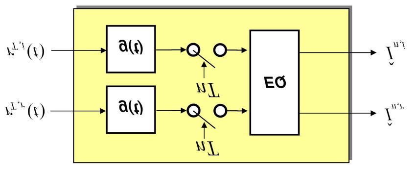
Figure 3.1 Equalizer structure on the receiving end in the baseband
The received high-frequency bandpass signal ( ) is given by the convolution of the channel
impulse response ( ) with the transmitted signal ( ), and an additive noise term ( ):
( ) ( ) ( ) ( ) (3.1)
The signal at the output of the quadrature demodulator is accordingly a baseband signal
( ) ( ) ( ). With the aid of a linear filter the signal-to-noise ratio of the
received baseband signal at the sampling point is maximized. This is achieved by
adjusting the impulse response of the filter ( ) to the impulse response of the pulse shaping
filter ( ).
( ) ( ) (3.2)
Filters which carry out this adjustment are designated as “matched filters.” Excitement of the
“matched filter” with the impulse response of the pulse shaping filter ( ) yields its
autocorrelation function ( ) at the output of the “matched filter.” Provided that the
impulse response of the pulse shaping filter fulfills the Nyquist condition, for it holds:
( ) and ( ) . In the following a discrete-time signal model will be used, as
can be observed at the output of the “matched filter.” The symbol sequence is subsequently
convoluted with the discrete-time channel impulse response and added to the discrete-time
noise . Consequently, the discrete baseband signal applies to the input of the equalizer:
133.1 Zero-Forcing Equalization
(3.3)
The equalized sequence of modulation symbols in Figure 3.1 is determined by filtration of
the sampled baseband signal with the impulse response of the equalizer :
̂ (3.4)
(3.5)
The first term is deterministic and can be precisely calculated. The noise part, by comparison,
is a random quantity, from which merely statistical characteristics can be determined.
3.1 Zero-Forcing Equalization
The purpose of zero-forcing equalization is to completely eliminate channel corruption.
Additive noise influence is therefore not considered. The elimination of the channel
corruption means as a result that the convolution of the discrete channel impulse response
with the impulse response of the ZF equalizer yields a Dirac impulse. The discrete impulse
response is determined by channel estimation and is therefore known in the receiver. The
only unknown is the impulse response of the equalizer, whose equalizing coefficients are
determined by the following equation:
(3.6)
In this course a maximum of 3 coefficients ( ) will be used. Furthermore, a
dominant line-of-sight connection is assumed ( ). The following matrix representation
can be drawn upon for the calculation of the 3 equalizing coefficients:
[ ] [ ] [ ] (3.7)
3.2 Minimum Mean Square Error Equalization
The Minimum Mean Square Error (MMSE) Equalization coefficient is by this equalizer so
devised, that the mean square error between the transmitted modulation symbols and the
estimated symbol ̂ at the equalization output is minimal. The error is described as
follows:
̂ (3.8)
For the minimization the following criterion is provided:
143 Equalization
( | | ) ( | ̂| ) (3.9)
The realization of this requirement as well as the determination of the equalizing coefficient
is achieved with the following equation:
( [ ]) [ ] [ ] (3.10)
whereby describes the autocorrelation matrix of the channel impulse response .
( ) ( ) ( )
( ) ( ) ( )
[ ] (3.11)
( ) ( ) ( )
3.3 Baseband vs. Bandpass Signal
The correlation between baseband and bandpass domain is especially important by channel
measuring. A signal, which is transmitted over a frequency selective channel, experiences
intersymbol interference (ISI). In order to reverse such interference the received signal must
be equalized. In this course this is realized with the ZF, respectively MMSE equalizer. The
channel estimation plays a big role, for the more precisely the channel can be estimated, the
more effectively the ISI can be eliminated. Since the equalization of the received signal takes
place in the baseband, the estimated channel impulse response must exist in the baseband.
The bandpass signal ( ) is received in the receiver:
( ) ( ) ( ) ( ) (3.12)
This correlation is equivalently formulated in the baseband:
( ) ( ) ( ) ( ) ( ) ∑ ( ) (3.13)
With the aid of Equation 3.13 it can be shown that for all the channel impulse
response ( ) in the baseband domain is complex-valued, since in general the symbol
duration corresponds to a multiple of the period of the carrier frequency ⁄ . It
follows that the equalizing coefficients are also complex-valued. The channel impulse
response ( ), on the other hand, is purely real for all .
Tip: In this course purely real channel impulse responses with are considered.
153.4 Preparatory Problems
3.4 Preparatory Problems
Problem 6
The following channel impulse response is given:
( ) ( ) ( ) ( )
For the equalization a zero-forcing equalizer with 3 coefficients should be utilized. Determine
the equalizing coefficients . How great is the residual error?
Problem 7
The following channel impulse response is given:
( ) ( ) ( ).
For the signal equalization a MMSE equalizer with 5 coefficients
should be utilized. A signal to noise ratio of is given. Determine the MMSE
equalizing coefficients.
164 Design of the Experiment
4.1 Model
For the execution of the experiment a computer and a signal processing system are used. The
signal processor is a developmental module EVM56303 from Freescale. Using a menu
program on the signal processor system the experiment sequence can be controlled and the
various problems can be set. Furthermore all parameters necessary for the experiment (e.g.
coefficient sets of the equalizer) are adjustable with an incremental encoder. All algorithms
necessary for each point of the experiment are digitally processed in the signal processor
system (DSP56303). The output, however, will be analog. The carrier frequency is set to:
A principal overview circuit diagram of the experiment set-up (signal processor system) is
given in Figure 4.1.
Figure 4.1 Block circuit diagram of the experiment set-up
The input bit sequence is a binary pseudo-random source, which sends out a series of 0’s and
1’s. This simulates a digital signal to be transmitted to a receiver.
174.2 Experiment
4.2 Experiment
4.2.1 Evaluation of Various Modulations
This first part of the experiment pertains to finding out which modulations Mod1, Mod 2,
and Mod 3 are. To that end load the program in the menu under Modulation and alternate
between the submenus of the various modulations. For the triggering of the signal an external
trigger signal is used, which is found on the back of the device.
The following part problems should be answered for each kind of modulation.
Problem 1
a) Begin with Mod1 and display the modulation at the output of the quadrature
modulator on the oscilloscope. To trigger the signal an external trigger can be found
on the back of the device.
b) How can the modulation be determined by using the phase jump? Which phase jumps
and amplitude values result here?
c) Various digital modulation methods have been presented in this script. Which of these
modulation methods is applicable here?
d) Does a baseband or a bandpass signal apply here?
e) Does the signal have a carrier frequency? If yes, then specify it.
f) Determine the length of a transmitted symbol. How many periods does a symbol
comprise?
g) Determine the bandwidth of the signal.
h) What does the corresponding constellation diagram look like? Sketch it.
i) Think of a reasonable symbol bit assignment and draw the baseband signal of the
corresponding modulation for the bit sequence: 110010101110.
184 Design of the Experiment
4.2.2 Channel Measurement
In this part the transmission channel between the transmitter and receiver shall be determined.
For this purpose load the program in the menu under Kanalvermessung. The signal
( ( )) will be transmitted over the channel with a frequency . Various frequencies
{ } can be tuned using the incremental encoder, which can be displayed
on the screen. No external trigger signals are required for this experiment.
Problem 2
a) Can the transfer function ( ) be determined from the time domain with this
procedure? Justify your answer.
b) Display the transmitted signals for various frequencies at the input of the receiver
on the oscilliscope. Sketch the absolute value of the transfer function | ( )| using the
received signals. (round to one decimal)
c) Determine the impulse response ( ) using the measured absolute value frequency
response | ( )|. Hint: The channel impulse response possesses 2 echoes of the form:
( ) ( ) ( ) ( )
Determine using the measured absolute value frequency response | ( )|.
Think about what influence the individual echoes in the time domain exert on the
frequency domain. Choose the frequencies such that the calculations can be
drastically simplified Simplification: the echoes occur as multiples of the symbol
duration .
d) Does the transmission channel exhibit nearly frequency-selective behavior? What is
the frequency selectivity determined by? Justify your answer.
194.2 Experiment
4.2.3 Signal Equalization
In this part the received signal shall be equalized. For this purpose the ZF equalizer with three
coefficients is considered. Load the program in the menu under Entzerrung.
Problem 3
a) Load the program and set some initial arbitrary values for . What do you
observe at the equalizer output? (Vary the S/N ratio also)
b) In the previous exercise you determined the channel impulse response ( ).
Determine the ZF equalizer coefficients using your result.
c) Set the equalizer coefficient on the display using the incremental encoder and load the
coefficients in the ZF equalizer. What do you observe at the equalizer output now?
Load the program in the menu under Rauschanteil for the transmission path.
Various SNR values [ ] can be set using the incremental encoder.
d) What do you observe at the equalizer output by low SNR values? By high SNR
values? Describe this effect.
Problem 4
Repeat exercises a), c) and d) from Problem 3 for the MMSE equalizer with MMSE equalizer
coefficients .
a) Determine the MMSE equalizer coefficient for . The use of Matlab is
allowed for the calculation.
b) How does the MMSE equalizer differ from the ZF equalizer?
20Important Formula symbols
() information carrying variable
sampling frequency
carrier frequency
constellation point
( ) modulation impulse
real part of the baseband signal
imaginary part of the baseband signal
bit sequence
( ) complex-valued baseband signal
( ) real-valued bandpass signal
time delay
maximum time delay
( ) Dirac impulse
symbol duration
control variable for the designation of the value sequence in the time
interval of the carrier frequency
control variable for the designation of the value sequence in the time
interval of the sampling frequency
( ) channel impulse response in bandpass domain
( ) channel impulse response in baseband domain
21Bibliography
[Qur85] S.U.H. Qureshi: Adaptive equalization, Proceedings of the IEEE, Volume 73,
Issue 9, Sept. 1985 pp:1349 - 1387
[Pro08] J.G. Proakis, M. Salehi: Digital Communications, 5th edition, McGraw-Hill,
2008
[Skl01] B. Sklar: Digital Communications-Fundamentals and Applications, 2nd
edition, Prentice Hall, 2001
[Rup82] W. Rupprecht, K. Steinbuch: Nachrichtentechnik, Band 2:
Nachrichtenübertragung, Berlin/Heidelberg/New York, 1982
[Lük07] H.D. Lüke: Signalübertragung, Berlin/Heidelberg/New York: Springer-
Verlag, 2007, 10. Auflage
[Sch84] H.W. Schüßler: Netzwerke, Signale und Systeme, Berlin/Heidelberg/New
York: Springer-Verlag, 1984
[Boc83] P. Bocker: Datenübertragung, Band 1: Grundlagen, Berlin/Heidelberg/New
York/Tokyo: Springer-Verlag, 1983
[Azi83] S.A. Azizi: Entwurf und Realisierung digitaler Filter, München/Wien, R.
Oldenbourg Verlag, 1983
[Kam80] K.D. Kammeyer, H. Schenk: Digitale Modems zur schnellen
Datenübertragung über Fernsprechkanäle (ausgewählte Arbeiten über
Nachrichtensysteme Nr. 39), herausgegeben von Prof. Dr.-Ing. H.W. Schüßler,
Erlagen, 1980
22You can also read