Discovery and mass measurement of the hot, transiting
←
→
Page content transcription
If your browser does not render page correctly, please read the page content below

A&A 659, A17 (2022)
https://doi.org/10.1051/0004-6361/202142653                                                                            Astronomy
                                                                                                                        &
© ESO 2022
                                                                                                                       Astrophysics

            Discovery and mass measurement of the hot, transiting,
                        Earth-sized planet, GJ 3929 b?
   J. Kemmer1, ?? , S. Dreizler2 , D. Kossakowski3 , S. Stock1 , A. Quirrenbach1 , J. A. Caballero4 , P. J. Amado5 ,
             K. A. Collins6 , N. Espinoza7 , E. Herrero8,9 , J. M. Jenkins10 , D. W. Latham6 , J. Lillo-Box4 ,
         N. Narita11,12,13 , E. Pallé13,14 , A. Reiners2 , I. Ribas8,9 , G. Ricker15 , E. Rodríguez5 , S. Seager15,16,17 ,
       R. Vanderspek15 , R. Wells18 , J. Winn19 , F. J. Aceituno5 , V. J. S. Béjar13,14 , T. Barclay20,21 , P. Bluhm1,?? ,
      P. Chaturvedi22 , C. Cifuentes4 , K. I. Collins23 , M. Cortés-Contreras4 , B.-O. Demory18 , M. M. Fausnaugh15 ,
A. Fukui11,13 , Y. Gómez Maqueo Chew24 , D. Galadí-Enríquez25 , T. Gan26 , M. Gillon27 , A. Golovin1,?? , A. P. Hatzes22 ,
    Th. Henning3 , C. Huang15 , S. V. Jeffers28 , A. Kaminski1 , M. Kunimoto15 , M. Kürster3 , M. J. López-González5 ,
         M. Lafarga8,9,29 , R. Luque5 , J. McCormac29 , K. Molaverdikhani30,31,1 , D. Montes32 , J. C. Morales8,9 ,
     V. M. Passegger33,34 , S. Reffert1 , L. Sabin35 , P. Schöfer2 , N. Schanche18 , M. Schlecker3 , U. Schroffenegger18 ,
                     R. P. Schwarz36 , A. Schweitzer33 , A. Sota5 , P. Tenenbaum37,10 , T. Trifonov3 ,
                                           S. Vanaverbeke38,39 , and M. Zechmeister2
                                                     (Affiliations can be found after the references)

                                               Received 12 November 2021 / Accepted 13 January 2022

                                                                       ABSTRACT

      We report the discovery of GJ 3929 b, a hot Earth-sized planet orbiting the nearby M3.5 V dwarf star, GJ 3929 (G 180-18, TOI-
      2013). Joint modelling of photometric observations from TESS sectors 24 and 25 together with 73 spectroscopic observations from
      CARMENES and follow-up transit observations from SAINT-EX, LCOGT, and OSN yields a planet radius of Rb = 1.150 ± 0.040 R⊕ , a
      mass of Mb = 1.21 ± 0.42 M⊕ , and an orbital period of Pb = 2.6162745 ± 0.0000030 d. The resulting density of ρb = 4.4 ± 1.6 g cm−3
      is compatible with the Earth’s mean density of about 5.5 g cm−3 . Due to the apparent brightness of the host star (J = 8.7 mag) and
      its small size, GJ 3929 b is a promising target for atmospheric characterisation with the JWST. Additionally, the radial velocity
      data show evidence for another planet candidate with P[c] = 14.303 ± 0.035 d, which is likely unrelated to the stellar rotation period,
      Prot = 122 ± 13 d, which we determined from archival HATNet and ASAS-SN photometry combined with newly obtained TJO data.
      Key words. planetary systems – techniques: radial velocities – techniques: photometric – stars: individual: GJ 3929 –
      stars: late-type – planets and satellites: detection

1. Introduction                                                                measurements for planets on both sides of the gap confirmed
                                                                               their differing nature: dense and presumably rocky super-Earths
The Transiting Exoplanet Survey Satellite (TESS; Ricker et al.                 with smaller radii and low-density enveloped mini-Neptunes
2015) has led to the discovery and characterisation of a multitude             with larger radii (e.g. Rogers 2015; Jontof-Hutter 2019; Bean
of small exoplanets. This growth was facilitated by the inten-                 et al. 2021, and references therein). However, it is not clear
sive spectroscopic follow-up in order to measure radial velocities             which formation mechanisms lead to these distinct planet
(RVs) of the TESS objects of interest (TOI; Guerrero et al. 2021)              types.
and, thus, confirm their planetary nature by measuring their                       For example, rocky super-Earths could be created by photo-
masses. (e.g. Cloutier et al. 2019; Günther et al. 2019; Luque                 evaporation (Owen & Wu 2013, 2017) or core-powered mass
et al. 2019; Astudillo-Defru et al. 2020; Dreizler et al. 2021;                loss (Ginzburg et al. 2018; Gupta & Schlichting 2019) of mini-
Kemmer et al. 2020; Nowak et al. 2020; Stefánsson et al. 2020;                 Neptunes with hydrogen-dominated atmospheres. The upper
Soto et al. 2021; Bluhm et al. 2020, 2021). These discoveries                  radius and mass limit of the rocky planets and its dependency
provide valuable data in the ongoing debate as to the origins of               on the planet’s period, or rather instellation, are often seen as
super-Earths and mini-Neptunes.                                                evidence for this theory (e.g. van Eylen et al. 2018, 2021; Bean
    The so-called radius gap, first observationally shown by                   et al. 2021, and references therein). On the other hand, the grow-
Fulton et al. (2017), divides the transiting sub-Neptunian                     ing number of planets residing in the gap pose a challenge to
planets into two different populations. Complementary mass                     this, since their high instellation usually excludes substantial H-
 ?
   RV data and stellar activity indices are only available at the CDS          He atmospheres (e.g. Ment et al. 2019; Dai et al. 2019; Bluhm
via anonymous ftp to cdsarc.u-strasbg.fr (130.79.128.5) or via                 et al. 2020). A possible explanation would be the existence of
http://cdsarc.u-strasbg.fr/viz-bin/cat/J/A+A/659/A17                           “water planets”, which were predicted by classical planet forma-
 ??
    Fellow of the International Max Planck Research School for Astron-         tion models (e.g. Bitsch et al. 2019). In fact, self-consistent planet
omy and Cosmic Physics at the University of Heidelberg (IMPRS-HD).             formation models, such as those by Venturini et al. (2020a,b),

                                                             Article published by EDP Sciences                                     A17, page 1 of 23
A&A 659, A17 (2022)

Table 1. Summary of transit observations.

Telescope                     Date                Filter texp          Airmass (a)    Duration (b) Nobs Aperture 10-min rms De-trending
                                                         (s)                            (min)            (pix)      (ppt)
TESS S24   2020-04-16 to 2020-05-12                 T        120           ...           38 138     14650       16          0.64          PDC
TESS S25   2020-05-14 to 2020-06-08                 T        120           ...           36 967     17 246      17          0.63          PDC
OSN              2021-03-14                       None       30    1.05→1.00→1.02         145        182        22          0.72         Airmass
SAINT-EX         2021-03-20                      I + z (c)    10    1.64→1.0→1.05         334        638        11          2.19           PCA
LCOGT McD        2021-04-10                         z0s       40       1.54→1.02          183        158        19          0.95      totc, width (d)
LCOGT CTIO       2021-04-10                         z0s       40   2.89→2.40→2.84         203        175        19          1.31      totc, width (d)
LCOGT HAL        2020-04-15                         g0       180   1.10→1.03→1.14         203        101        20          1.17       totc, b jd (d)
LCOGT HAL        2020-04-15                         r0        38   1.10→1.03→1.14         206        286        20          0.71       totc, b jd (d)
LCOGT HAL        2020-04-15                         i0        25   1.10→1.03→1.14         205        403        20          0.68       sky, b jd (d)
LCOGT HAL        2020-04-15                         z0s       21   1.10→1.03→1.14         207        510        20          0.62      width, b jd (d)
OSN              2021-05-16                       None       30        1.23→1.00          180        297        22          0.55         Airmass
OSN              2021-07-02                       None       30        1.03→2.53          275        452        22          1.18         Airmass
OSN              2021-08-13                       None       30        1.10→1.60          138        229        22          1.05         Airmass

Notes. (a) The arrows indicate how the airmass has changed over the observation. (b) Time span of the observation. (c) Combined range (d) simultaneous
to the fits. Explanation of de-trending parameters: totc ≡ comparison ensemble counts; width ≡ full width at half maximum (FWHM) of the target;
b jd ≡ BJD timestamp of observation; sky ≡ sky background brightness.

predict a bimodal distribution, with purely rocky planets on                  2. Data
one side and water-enriched planets on the other. Probing the
atmospheres of mini-Neptunes will break the density degeneracy                2.1. High-resolution spectroscopy
between H-He atmospheres and water planets and provide                        We took 78 observations of GJ 3929 between July 2020 and July
more insight (Rogers & Seager 2010; Lopez & Fortney 2014;                     2021 with CARMENES1 (Quirrenbach et al. 2014) in the course
Zeng et al. 2019). The position of the radius gap, anchored by the            of the guaranteed time observation and legacy programmes.
distribution of planets on both sides, is also a probe for the under-         The dual-channel spectrograph covers the spectral ranges of
lying principles and an important input for theoretical models                0.52 µm–0.96 µm in the visible light (VIS; R = 94600) and
that aim to describe the formation and evolution of those planets             0.96 µm1.71 µm in the near infrared (NIR; R = 80 400). For
(Bean et al. 2021 and references therein).                                    the data reduction and extraction of the RVs, we used caracal
    Considered on their own, the planets below the radius gap are             (Caballero et al. 2016b) and serval (Zechmeister et al. 2018,
also interesting. For example, the increasing statistical sample of           2020), following our standard approach (e.g. Kemmer et al.
the smallest planets will tell us if super-Earths are different from          2020). The observations were taken with an exposure time of
planets with masses and radii similar to Earth, or if the under-              30 min, which resulted in a median signal-to-noise ratio (S/N)
lying formation mechanisms are the same. Related to this is the               of 74 (min. = 15, max. = 100). After discarding spectra with
question how abundant atmospheres with high mean-molecular-                   missing drift correction (i.e. without simultaneous calibration
weight similar to the ones that we observe in the Solar System                measurements from the Fabry-Pérot), we retrieved 73 RVs in
actually are. Particularly suited to answer those questions are the           the VIS with a median internal uncertainty of 1.9 m s−1 and a
planets orbiting M-dwarf stars, as these will be the first ones               weighted root mean square (wrms) of 4.0 m s−1 and 72 RVs in the
where the atmospheric characterisation of exo-Earths will be                  NIR with a median internal uncertainty of 7.3 m s−1 and wrms
possible and provide unique insight in their structure and com-               9.1 m s−1 in the NIR, respectively. Due to the large scatter of
position (e.g. Rauer et al. 2011; Barstow & Irwin 2016; Morley                the NIR data and the small expected amplitude of the transiting
et al. 2017; Kempton et al. 2018).                                            planet candidate, we only considered the VIS data in our analysis
    In this study, we present the discovery of a hot Earth-sized              (Bauer et al. 2020).
planet orbiting the M3.5 V-dwarf star, GJ 3929. Based on tran-
sit signals observed by TESS, we performed an intensive RV
follow-up campaign with CARMENES to confirm its plane-                        2.2. Transit photometry
tary origin. The characterisation of the planet was supported
by photometric follow-up from SAINT-EX, LCOGT, and OSN                        For our analysis, we combined the TESS observations with
that helped to refine the transit parameters. Furthermore, we                 ground based follow-up transit photometry obtained by the TESS
report the detection of a non-transiting, sub-Neptunian-mass                  follow-up observing programme sub-group one. The parameters
planet candidate with a wider orbit, which is evident in the RV               of the used transit observations are summarised in Table 1. In
data.                                                                         the following, we provide an overview of the instruments and
    Our paper is organised as follows. In Sect. 2, we present the             applied data reduction.
data used, and in Sect. 3 we describe the stellar properties of
GJ 3929. Data analysis is described in Sect. 4, and our findings              1 Calar Alto high-Resolution search for M dwarfs with Exoearths with
are discussed in Sect. 5. Finally, Sect. 6 gives a summary of our             Near-infrared and visible Echelle Spectrographs, http://carmenes.
results.                                                                      caha.es

A17, page 2 of 23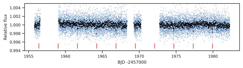
J. Kemmer et al.: Discovery of a planetary system around GJ 3929

Fig. 1. TESS PDCSAP light curves for sector 24 (top) and sector 25 (bottom). The blue points are the measurements and the black dots are 20 min
bins. The transit times of GJ 3929 b are indicated by red ticks.

2.2.1. TESS                                                               steps including bias, dark, and flat-field correction and provides
                                                                          light curves obtained from differential photometry (Demory
We retrieved TESS observations for GJ 3929 (TOI 2013) from                et al. 2020). The light curve used for our analysis was further
the Mikulski Archive for Space Telescopes2 for the two sec-               corrected for systematics using a principle component analysis
tors 24 and 25 (see Fig. 1). In sector 24 (camera #1, CCD #1),            (PCA) method based on the light curves of all suitable stars in
one transit event was not observed because of the interrup-               the FOV except for the target star (Wells et al. 2021).
tion during the data downlink between BJD = 2458968.35 and
BJD = 2458969.27. In sector 25 (Camera #1, CCD #2), the
measurements were stopped for data download between BJD =                 2.2.3. LCOGT
2458995.63 and BJD = 2458996.91, which led to one, only                   Two transit events were observed with instruments from the
partially observed, transit. We used the pre-search data condi-           LCO4 global telescope network (LCOGT; Brown et al. 2013).
tioning simple aperture photometry (PDCSAP; Smith et al. 2012;            The first one was observed contemporaneously by the SIN-
Stumpe et al. 2012, 2014) light curves provided by the Science            ISTRO CCDs at the 1 m telescopes of the McDonald Obser-
Processing Operations Center (SPOC; Jenkins et al. 2016), which           vatory (McD) and the Cerro Tololo Interamerican Observatory
are based on simple aperture photometry (SAP) light curves,               (CTIO). Both instruments have a pixel scale of 0.00 389 pix−1 and a
but further corrected for instrument characteristics. The aper-           FOV of 260 × 260 . However, the higher airmass at LCOGT CTIO
ture masks used for retrieving the SAP light curves are shown             (see Table 1) led to worse seeing (estimated point spread func-
in Fig. 2. To reduce the computational cost of the analysis, we           tion size 5.00 34 pix−1 vs. 3.00 97 pix−1 ) and, therefore, larger scatter
used the extracted transit events only. In doing so, the baseline         of the measurements. The second transit event was observed
for each transit was set to ±3 h with respect to the expected times       by the recently commissioned MuSCAT35 camera (Narita et al.
of transit centre.                                                        2020) mounted on the 2 m Faulkes Telescope North at Haleakalā
                                                                          Observatory (HAL). MuSCAT3 operates simultaneously in the
2.2.2. SAINT-EX                                                           four passbands, g0 , r0 , i0 , and z0s , and has a pixel scale of
                                                                          0.00 27 pix−1 corresponding to a FOV of 9.0 1 × 9.0 1. All LCOGT
The first follow-up transit photometry for GJ 3929 was taken              observations were calibrated by the standard LCOGT BANZAI
with the SAINT-EX3 telescope located at the Observatorio                  pipeline (McCully et al. 2018a,b), and photometric data were
Astronómico Nacional in the Sierra de San Pedro Mártir in                 extracted using AstroImageJ (Collins et al. 2017).
Baja California, Mexico. SAINT-EX consists of an Andor iKon-
L camera mounted to an 1 m f /8 Ritchey–Chrétien telescope
with a pixel scale of 0.00 34 pix−1 , which corresponds to a field        2.2.4. OSN
of view (FOV) of 120 × 120 (Demory et al. 2020). The reduc-               We detected four transit events with the 90 cm Ritchey–Chrétien
tion of the data was performed using the instrument’s custom              telescope of the Observatorio de Sierra Nevada (OSN). The
pipeline, prince, which performs the standard image reduction
                                                                          4  Las Cumbres Observatory.
2   https://mast.stsci.edu                                                5  Multicolor Simultaneous Camera for studying Atmospheres of Tran-
3   Searching and characterising transiting exoplanets.                   siting exoplanets 3.
                                                                                                                                 A17, page 3 of 23
A&A 659, A17 (2022)
12 3.0
2.5 a pixel scale of 1400 pix−1 . We retrieved the observations cover-
1196 m= 5 2.0 ing a time span of 200 d between December 2004 and July 2005
m= 6 1.5
1.0 from the NASA Exoplanet Archive6 . The data were taken by tele-
m= 7 scopes #9 and #11 in the Cousins Ic filter at the Fred Lawrence
1194 m= 8 0.5 Whipple Observatory in Arizona. Originally, the data were taken
Pixel Row Number
Flux ×103 (e )
with a cadence of 5.5 min, but for our search for long-periodic
1192 9 signals we used the nightly binned values. In this way, we obtain
1 a mean uncertainty of 1.24 ppt and rms of 2.19 ppt.
11 4 6
1190
5 2 3 10 2.3.2. ASAS-SN
1188 We obtained more than 5 yr of archival data from ASAS-SN
87 E 0.0
(Shappee et al. 2014; Kochanek et al. 2017), which were taken
N between April 2013 and September 2018. ASAS-SN currently
1186 consists of 24 cameras mounted on the 14 cm Nikon telephoto
1602 1600 1598 1596 1594 1592 lenses at six different sites around the globe. Each unit has a
Pixel Column Number FOV of 4◦.5 × 4◦.5 with a pixel scale of 8.00 0 pix−1 . The observa-
tions of GJ 3929 were obtained in the V band with the second
894 11 2.5 camera in Hawai’i and have a mean uncertainty of 4.82 ppt and
m= 5 2.0
1.5 rms of 6.68 ppt.
m= 6 1.0
892 m= 7
m= 8 0.5 2.3.3. TJO
Pixel Row Number
Flux ×103 (e )
890 8 We observed GJ 3929 from April to October 2021 with the 0.8 m
4 Joan Oró telescope (TJO; Colomé et al. 2010) at the Montsec
1 10 Observatory in Lleida, Spain. We obtained a total of 593 images
888 with an exposure time of 60 s using the Johnson R filter of the
9
2 3 LAIA imager, a 4k × 4k CCD with a field of view of 300 and
886 a scale of 0.00 4 pix−1 . The images were calibrated with darks,
12 5 bias, and flat fields with the icat pipeline of the TJO (Colome
76 E 0.0 & Ribas 2006). The differential photometry was extracted with
884 AstroImageJ using the aperture size that minimised the rms of
N the resulting relative fluxes, and a selection of the ten brightest
2076 2074 2072 2070 2068 2066 comparison stars in the field that did not show variability. Then,
Pixel Column Number we used our own pipelines to remove outliers and measurements
affected by poor observing conditions or presenting a low signal-
Fig. 2. TESS TPFs of GJ 3929. Top: TESS sector 24, bottom: TESS to-noise ratio. For our analysis, we binned the data nightly, which
sector 25. The position of GJ 3929 is denoted by a white cross, and the resulted in a total of 54 measurements with a mean uncertainty
aperture mask used to create the PDCSAP light curves is shown as the of 1.90 ppt and rms of 6.22 ppt.
pixels with orange borders. For comparison, nearby sources from
the Gaia DR2 catalogue (Gaia Collaboration 2018), up to a difference
of ∆m = 8 mag in brightness compared to GJ 3929, are plotted by red 2.4. High-resolution imaging
circles. Figure created using tpfplotter (Aller et al. 2020).
We observed GJ 3929 with the high-spatial resolution camera
AstraLux (Hormuth et al. 2008), which is located at the 2.2 m
telescope is equipped with a 2k × 2k CCD camera with a pixel telescope of the Calar Alto Observatory (Almería, Spain). The
scale of 0.00 4 pix−1 that provides a FOV of 13.0 2 × 13.0 2 (Amado observations were carried out on 7 August 2020 at an airmass of
et al. 2021). All frames were corrected for bias and flat-fielding, 1.1 and under moderate weather conditions with a mean seeing
and the light curves were obtained using synthetic aperture pho- of 1.00 1. In total, we obtained 93 700 frames in the Sloan Digi-
tometry. Outliers due to bad weather or very high airmass were tal Sky Survey z0 filter (SDSSz) with 10 ms exposure times and
removed from the dataset. The light curves were de-trended windowed to a FOV of 600 × 600 . We used the instrument pipeline
before the fitting using the airmass in a linear fit. to select the 10 % frames with the highest Strehl ratio (Strehl
1902) and to combine them into a final high-spatial-resolution
2.3. Long-term photometry image. Based on this final image, a sensitivity curve was com-
puted using our own developed astrasens7 package (Lillo-Box
In addition to the photometric transit observations, we used long- et al. 2012, 2014).
term photometry to determine the stellar rotation period.
3. Properties of GJ 3929
2.3.1. HATNet
The star GJ 3929 (G 180-18, Karmn J15583+354) is located at
The photometric variability of GJ 3929 was previously inves-
a distance of only 15.830 ± 0.006 pc and shows a high proper
tigated by Hartman et al. (2011) using data from the HATNet
telescope network (Bakos et al. 2004, 2006). HATNet comprises 6 https://exoplanetarchive.ipac.caltech.edu/docs/
a network of six cameras attached to 11 cm telescopes located in datasethelp/ETSS_HATNet.html
Arizona and Hawai’i. The cameras have a FOV of 8◦.2 × 8◦.2 and 7 https://github.com/jlillo/astrasens
A17, page 4 of 23J. Kemmer et al.: Discovery of a planetary system around GJ 3929
motion (Schneider et al. 2016; Gaia Collaboration 2018). Lépine Table 2. Stellar parameters of GJ 3929.
et al. (2013) classified the star as an M3.5 V red dwarf. We cal-
culated homogeneous stellar parameters from the CARMENES
Parameter Value Ref.
high-resolution spectra using our standard method: the luminos-
ity, L? = 0.01155 ± 0.00011 L , was determined in Cifuentes Name and identifiers
et al. (2020). Following Passegger et al. (2019), and assuming Name GJ 3929 Gli91
v sin i = 2 km s−1 , we derived the effective temperature, T eff = Alternative name G 180–18 Gic59
3369 ± 51 K, surface gravity log g = 4.84 ± 0.04 dex, and metal- Karmn J15583+354 Cab16
licity [Fe/H] = 0.00 ± 0.16 dex using the VIS spectra8 . Finally, TIC 188589164 Stas19
we computed the stellar radius, R? = 0.315 ± 0.010 R , using TOI 2013 Gue21
the Stefan-Boltzman law, and, consequentially, the mass, M? = Gaia EDR3 1372215976327300480 Gaia EDR3
0.309 ± 0.014 R , from the empirical mass-radius relation for M
Coordinates, magnitudes, and spectral type
dwarfs of Schweitzer et al. (2019). Additionally, we computed
galactocentric space velocities UVW as in Cortés-Contreras α (epoch 2016.0) 15 58 18.80 Gaia EDR3
(2017). δ (epoch 2016.0) +35 24 24.3 Gaia EDR3
From the analysis of the Hα pseudo-equivalent width (pEW), Spectral type M3.5 V Lép13
we found that GJ 3929 is an Hα-inactive star and is consistent T (mag) (a) 10.2705 ± 0.0074 Stas19
with the previous results of Schöfer et al. (2019) and Jeffers Parallax and kinematics
et al. (2018). In addition, we investigated if there are any cor- µα cos δ (mas yr−1 ) −143.06 ± 0.02 Gaia EDR3
relations between the measured CARMENES RV values and all
µδ (mas yr−1 ) 318.12 ± 0.03 Gaia EDR3
of the activity indices using the Pearson’s r coefficient where
π (mas) 63.173 ± 0.020 Gaia EDR3
a value of >0.7 orA&A 659, A17 (2022)
Planet parameters. Based on the analysis of the TESS light
2 2 curves by the SPOC pipeline (Li et al. 2019), the transiting planet
Contrast (SDSSz) [mag]
1 candidate has a period of 2.616277 ± 0.000113 d. We used this
[arcsec]
information to set a uniform prior between 2 d to 3 d for our
3 0 analysis. The time-of-transit centre was chosen accordingly to
be uniform between BJD 2459319.0 d to 2459322.0 d, which
4 -1 comprises the decently resolved follow-up transit observed by
LCOGT-HAL. Following our usual approach (e.g. Luque et al.
-2 2019; Kemmer et al. 2020; Bluhm et al. 2021), we fitted for the
5 -2 -1 0 1 2 stellar density, ρ∗ , instead of the scaled planetary semi-major
[arcsec] axis, a/R∗ . In doing so, we used a normally distributed prior cen-
6 tred on the density calculated from the parameters in Table 2.
For this, we assigned a width of three times the propagated
0.0 0.5 1.0 1.5 2.0 uncertainty. Furthermore, we implemented the re-parameterised
fit variables r1 and r2 , which replace the planet-to-star radius
Separation [arcsec] ratio, p, and the impact parameter, b, and allow for a uniform
Fig. 3. Contrast curve of the AstraLux high-resolution image. The sampling between zero and one (Espinoza 2018). Since the infor-
image used to create the contrast curve is shown in the inset. mation content regarding the eccentricity is rather small for the
light curves (Barnes 2007; Kipping 2008; van Eylen & Albrecht
2015), we assumed it to be zero for the transit-only modelling.
during commissioning and early science operations. Neverthe- Constraints on the eccentricity were later investigated using the
less, we obtained additional lucky imaging observations to rule RV data (see Sect. 4.5).
out contamination of the light curves by bound or unbound com-
panions at sub-arcsecond separations (Sect. 2.4). The AstraLux Instrument parameters. The analysis of the high-resolution
image of GJ 3929 and the contrast curve created from it are images (Sect. 4.2) did not indicate any contaminating sources
shown in Fig. 3. We find no evidence of additional sources within within the apertures that were used to generate the light curves.
this FOV and within the computed sensitivity limit. This allows Therefore, the dilution factor was fixed to 1 for all instruments.
us to set an upper limit to the contamination in the light curve of Following Espinoza & Jordán (2015), we used a quadratic limb-
around 0.4% down to 0.00 4 and 2.5% down to 0.00 2. darkening law for the space-based TESS light curves, parame-
Analogously to Lillo-Box et al. (2014), we further used the terised by q1 and q2 as in Kipping (2013). The parameters were
contrast curve to estimate the probability of contamination from shared between the two sectors. For all the other ground-based
blended sources in the TESS aperture based on the TRILEGAL9 follow-up observations, we assumed a linear limb darkening
Galactic model (v1.6, Girardi et al. 2012). The transiting planet with coefficient q. The offsets between the instruments, m f lux,
candidate around GJ 3929 produces a signal that could be mim- were assumed to be normally distributed around 0 with a stan-
icked by blended eclipsing binaries with magnitude contrasts up dard deviation of 0.1, whereas the additional scatter that was
to ∆mb,max ≈ 7.3 mag in the SDSSz passband. Translating this added in quadrature to the nominal uncertainty values was log-
contrast results in a low probability of 0.1% for an undetected uniformly distributed between 0 ppm to 5000 ppm. The light
source, and an even lower probability of such a source being an curves from the LCOGT were de-trended simultaneously with
appropriate eclipsing binary. Given these numbers, we assumed the fits, whereas, following a preliminary analysis, de-trending
that the transit signal is not due to a blended binary star and that of the SAINT-EX light curve did not bring any improvement,
the probability of a contaminating source is nearly zero. which is why we refrained from doing so in the analysis. More-
over, the OSN light curves were de-trended before the fit as
4.3. Modelling technique described in Sect. 2.2. We invite the reader to consult Table 1 for
an overview of the used de-trending parameters of the individual
We used juliet10 (Espinoza et al. 2019) for the analysis and light curves. In this way, we determined a refined period of P =
modelling of the transit and RV data. Thereby, we follow our 2.6162733 ± 0.0000034 d and t0 = 2459320.05803 ± 0.00024 d
method as detailed for example by Luque et al. (2019), Kemmer from the fit.
et al. (2020), or Stock et al. (2020b). Because of the variety of In order to search for additional transit signals in the data,
instruments used and the large dataset, it would not be reasonable we applied the model from this fit to the entire TESS dataset
to perform the model selection on the combined RV and transit (i.e. uncropped) and ran a transit least squares (TLS; Hippke &
data. Therefore, in the following we first present transit-only and Heller 2019) periodogram on the residuals. The periodogram did
RV-only analyses to determine the individually best fitting mod- not show any further significant signals.
els, which were later combined into a joint fit to retrieve the most
precise parameters for the system.
4.5. RV-only modelling
4.4. Transit-only modelling
4.5.1. Periodogram analysis
In the first step of the modelling, we combined the TESS light
We used generalised Lomb-Scargle periodograms (GLS;
curves with the SAINT-EX, LCOGT, and OSN follow-up tran-
Zechmeister & Kürster 2009) implemented in Exo-Striker
sits to obtain a very precise updated ephemeris of the transiting
(Trifonov 2019; Trifonov et al. 2021) to identify prominent sig-
planet candidate, which was later used as prior information for
nals in the RV data, as illustrated by Fig. 4. The dominant period
the RV-only modelling.
is not that of the transiting planet candidate at about 2.6 d, but a
9 http://stev.oapd.inaf.it/cgi-bin/trilegal signal with periodicity of P ≈ 15 d and its one-day aliases. Fur-
10 https://juliet.readthedocs.io/en/latest/ thermore, aliasing due to the seasonal observability of GJ 3929
A17, page 6 of 23J. Kemmer et al.: Discovery of a planetary system around GJ 3929
Period [d] Period [d]
50 10 5 2 1
1.0 16.67 12.50 1.08 1.06 0.94 0.93
Window function
0.5
0.4
0.0
0.3 (O-C) 0P
0.2 0.2
0.1
0.3 (O-C) 1P (15 d) 0.0
Power (ZK)
Power (ZK)
0.2 0.06 0.08 0.930 0.945 1.065 1.080
0.1
0.3 (O-C) 2P (2.6 d, 15 d)
0.2 0.4
0.1
0.3 (O-C) 2P (2.6 d, 14.35 d) + dSHO-GP 0.2
0.2
0.1 0.0
0.06 0.08 0.930 0.945 1.065 1.080
0.0 0.2 0.4 0.6 0.8 1.0 1.2
Frequency f [1/d] Frequency f [1/d]
Fig. 4. GLS periodogram analysis of the RVs. In the first panel, we show Fig. 5. Alias test for the 14.3-day and 15.0-day periods using
the window function of the CARMENES data. In the subsequent pan- AliasFinder. We generated 5000 synthetic datasets for each period
els, the residuals after subtracting models of increasing complexity are to produce synthetic periodograms (black lines), which are compared
presented. The components that were considered for the fits are listed in with the periodogram of the observed data (red lines). The simulation
the inset texts (see also Table 3). The period, P = 2.62 d, and one-day for the 15.0-day signal is shown in the top row and the simulation for
alias, P = 1.62 d, of the transiting planet are marked by the red solid the 14.3-day signal in the bottom row, each period indicated by a verti-
and dashed lines, while the ∼15-day periodicity and its daily aliases are cal blue dashed line, respectively. Black lines depict the median of the
marked by blue solid and dashed lines, respectively. Additionally, even samples for each simulation, and the grey shaded areas are the 50, 90,
though insignificant in the periodogram, the stellar rotation period of and 99% confidence intervals. Furthermore, the phases of the peaks as
P = 122 d (Sect. 4.7) is indicated by the purple dot-dashed line. We nor- determined by the GLS periodogram are displayed in the circles, fol-
malised the power using the parametrisation of Zechmeister & Kürster lowing the same colour scheme (the grey shades denote the standard
(2009), and the 10, 1, and 0.1% FAPs denoted by the horizontal grey deviations of the simulated peaks). The black arrows point out the dif-
dashed lines were calculated using the analytic expression. ference in the periodograms for the daily aliases that allows to identify
the best matching period (see the text for the discussion).
( fs ≈ 1/292 d−1 ) splits the ∼15-day signal up into multiple close 4.5.2. Determining the true period underlying the ∼15 d GLS
peaks by itself. The two prominent peaks are thereby at periods peaks
of P ≈ 14.3 d and P ≈ 15.0 d (see also Sect. 4.5.2). As there are
no obvious indications of a transiting signal corresponding to We made use of the AliasFinder11 (Stock & Kemmer 2020;
these two periodicities that would help to distinguish the aliases, Stock et al. 2020a) to identify the true period underlying the GLS
we used a sinusoidal fit with an uninformative period bound- peaks of 14.3 d and 15.0 d, which are aliases of each other caused
ary between 10 d to 20 d to subtract the signal, and determined by the fs ≈ 1/292 d−1 sampling frequency. The script imple-
a period of P = 15.03 d. The residuals of this fit show a peak ments the principle of Dawson & Fabrycky (2010) and allows
with about a 2% false alarm probability (FAP) at a period of us to visually compare the observed periodogram with synthetic
P ≈ 1.62 d. This period corresponds to the one-day alias of the periodograms originating from different possible alias frequen-
2.62-day signal seen in the transits, which is itself apparent only cies. In doing so, we excluded the influence of the 2.62-day
as an insignificant signal in the GLS periodogram. The photo- signal by first removing it from the data with a sine fit, as we did
metric observations presented in the previous section, however, for the periodogram analysis. Fig. 5 shows the resulting compar-
supplied precise information on the period and transit time, and ison periodograms for the 14.3-day and 15.0-day periods. Each
hence phase, of the transiting planet candidate. We therefore panel shows three sections of the full periodogram; the first panel
simultaneously fitted the ∼15-day signal in combination with a is the region around ∼15 d, which highlights the aliasing due to
sinusoid of P ≈ 2.62 d, whose ephemeris was fixed to the values the ∼292 d sampling ( falias = | f ± 2921 d |), and the other two show
from Sect. 4.4. The residuals of this fit do not show any power at the aliases of the daily sampling (middle panel: falias = | f − 11d |),
the period of P ≈ 1.62 d, which confirms that the peak is indeed right panel: falias = | f + 11d |)). The idea behind this is that the true
correlated in phase with the signal of the transiting planet can- frequency should be able to explain both patterns well, as they
didate, and, thus, it is caused by aliasing. Even though never are generated independently by it.
significant, a peak near the stellar rotation period of 122 d is also
visible in the GLS periodograms (see Sect. 4.7). 11 https://github.com/JonasKemmer/AliasFinder
A17, page 7 of 23A&A 659, A17 (2022)
While the phases originating from the stimulation of the Table 3. Model comparison for RVs based on Bayesian log evidence.
15.0-day period show less deviations from the observed phases
than those from the 14.3-day period (see the circles in Fig. 5),
Model ln Z ∆ ln Z
the evaluation of the periodograms implies that 14.3 d is the
period underlying our data. The peaks originating from the 15.0- No planet
day period show a shifted distribution when compared to the 0P –213.3 –6.0
observed periodogram, which can be seen especially well in the
Two-signal models (without activity modelling)
daily aliases. There, the envelope of the aliases at ∼1.07 d is
shifted towards shorter periods, and those at ∼0.94 d are shifted 2P(2.6d,14.3d) –211.2 –3.9
towards longer periods -as is expected when the simulated period 2P(2.6d−ecc,14.3d) –211.8 –4.5
is larger than the underlying one (see the black arrows in Fig. 5). 2P2.6d,14.3d−ecc) –211.2 –3.9
The distribution of the simulated periodogram originating from 2P(2.6d−ecc,14.3d−ecc) –212.1 –4.8
the 14.3-day period, on the other hand, follows the observed peri- Three-signal models (with activity modelling)
odogram. This is also reflected by the rms power of the residuals 2P(2.6d,14.3d) + dSHO-GP(120d) −207.3 0.0
after subtracting the median GLS model from the observed one, 2P(2.6d−ecc,14.3d) + dSHO-GP(120d) –207.7 –0.4
where we found a value of 7.12 for the 14.3-day period and 7.97 2P(2.6d,14.3d−ecc) + dSHO-GP(120d) –208.0 –0.7
for the 15.0-day period. We also got the same result if we gener- 2P(2.6d−ecc,14.3d−ecc) + dSHO-GP(120d) –208.7 –1.4
ated the periodograms from the posterior samples of the fits, as
shown in Appendix A. Therefore, we concluded that the 14.3-day Notes. The bold font denotes the model that was used in the joint fit.
period is the true period of the ∼15-day signal, and adopted from
then on a uniform prior corresponding to the peak width in the
periodogram between 13.98 d to 14.71 d whenever this signal was
considered in a fit. Using the 14.3-day period for pre-whitening transiting planet. Therefore, we fixed the period and time-of-
the periodogram instead of the uninformative prior improved the transit centre for the first model component to the values from
FAP of the transiting planet candidate’s alias in the residual GLS the transit-only modelling (Sect. 4.4). This choice is justi-
periodogram to 0.8 %. fied because the precision of the transiting planet candidate’s
ephemerides as determined from the photometry is much higher
than what could be achieved from the RV data. To investigate the
4.5.3. Significance of the transiting planet candidate in the
eccentricity of the signal, we tested a sinusoid against a Keple-
RVs
rian model for the transiting
√ planet. Thereby, the
√ eccentricity was
In the next step, we derived the FAP for the signal in the RVs parameterised by S1 = e sin ω and S2 = e cos ω with uni-
to occur exactly at the period of the transiting planet candidate. form priors between –1 and 1 (Espinoza et al. 2019). The prior
One problem is the strong aliasing, which has the consequence of the RV amplitude of the signal was set uniformly between
that the 1.62-day alias of the transit signal has in fact the high- 0 m s−1 to 50 m s−1 .
est power in the periodogram. For our approach, we used the For the 14.3-day signal, we tested a sinusoidal or Kep-
randomisation method discussed by Hatzes (2019), Luque et al. lerian model in the same manner. The period prior was set
(2019), Kemmer et al. (2020), or Bluhm et al. (2021), where uniformly between 13.98 d to 14.71 d, following the analysis
the FAP is determined for increasingly smaller frequency ranges with AliasFinder in Sect. 4.5.2, and the time-of-transit cen-
around the period in question and extrapolated with a third-order tre was chosen uniformly between the first epoch of the RV data,
polynomial fit to a window size of zero. To account for the alias- 2459061.0 d, and 2459081.0 d to avoid a multi-modal distribution
ing in our case, we considered two windows that comprise the of the posterior.
two peaks at the periods of 2.62 d and 1.62 d in the periodogram We investigated whether the RVs are affected by stellar activ-
and compared their combined power with the combined power ity by adding a GP component whose prior on the rotation
of the respective highest peaks within the two windows. In period, PGP,rv , was set uniformly between 100 d to 150 d to cover
doing so, we found a FAP of 0.1% (Fig. B.1). We therefore con- the period determined from the photometry. Our GP kernel was
cluded that we detected a genuine signal of the transiting planet the sum of two simple harmonic oscillators kernels (Foreman-
candidate in the RV measurements. Mackey et al. 2017) as described in Kossakowski et al. (2021)
and hereafter called dSHO-GP (≡ double simple harmonic oscil-
lator). The prior on the standard deviation, σGP,rv , of the GP
4.5.4. Model comparison model was specified to be uniform between 0 m s−1 to 50 m s−1
following the Keplerian models. Moreover, we used a uniform
Planet and instrument parameters. The periodogram and prior between 0.1 and 1 for the fractional amplitude, fGP,rv , of
alias analysis showed two relevant periodicities in the RV data: the second component with respect to the first, and log-uniform
the strong signal at P ≈ 14.3 d and the transiting planet candidate priors between 1 ×10⁻¹ and 1 × 10⁴ for the quality factor of the
at P ≈ 2.62 d. As a result, the basis for our model comparison secondary component, Q0,GP,rv , and the difference compared to
is a “two-signal model”. Moreover, in Sect. 4.7 we determined the first component, dQGP,rv , respectively. For the instrumental
the stellar rotation period to be 122 d, which is recognisable as parameters of CARMENES, we used uniform priors between -
a peak in the periodogram of the RV data (Fig. 4), but not sig- 100 m s−1 to 100 m s−1 for the offset and 0 m s−1 to 100 m s−1 for
nificantly in terms of FAP. We took this into consideration for the jitter.
the modelling by testing whether an additional gaussian process
(GP) term that is optimised to mitigate stellar activity signals can Results. In Table 3, we show the Bayesian log evidence for
improve the fit (referred to as “three-signal models”). the models that combine the two signals from the periodogram
Based on the results from Sects. 4.2 and 4.5.3, we could and the stellar activity, as described above. The highest Bayesian
assume that the 2.62-day periodicity is indeed due to a true log-evidence was found for the model considering sinusoidal
A17, page 8 of 23J. Kemmer et al.: Discovery of a planetary system around GJ 3929
components for the 2.62-day and 14.3-day periods in combina- Table 4. Median posterior parameters of the transiting planet, the
tion with the GP that accounts for stellar activity. The difference ∼14.3 d signal, and the GP.
in log-evidence compared to a completely flat model, which
means considering only the RV offset and jitter, is |∆ ln Z| = 6. Parameter Posterior (a) Units
Following Trotta (2008), we thus assumed the three-signal model
to be significantly better (|∆ ln Z| > 5). Stellar density
In comparison with the two-signal models, the models that ρ? 14.96+0.47
−0.59 g cm−3
account for stellar activity are only moderately to almost signif- GJ 3929 b
icantly favoured (|∆ ln Z| > 2.5). The reason for this is probably −06
Pb 2.616 274 5+2.9×10 d
the low activity amplitude of ∼3 m s−1 combined with the fact −3.0×10−06
(b) 18
that only roughly three periods were covered by the RV obser- t0,b 2 459 320.058 08+0.000
−0.000 19 d
vations (∼350-day baseline compared to a period of ∼120 d). r1,b 0.405−0.046
+0.060
...
Nonetheless, considering that even small influences from stel- 41
r2,b 0.033 48+0.000
−0.000 41 ...
lar activity can affect the planetary parameters (e.g. Stock et al. Kb 1.23+0.40 m s−1
2020a), and that even strong activity signals do not have to be −0.43
evident in the periodogram (Nava et al. 2020), we proceeded 14.3 d signal
with the models that include the GP. P(14.3 d) 14.303+0.034
−0.035 d
Of these models, those that consider eccentric orbits for one t0,(14.3 d) (b)
2 459 072.44+0.41 d
of the two signals are at best indistinguishable (|∆ ln Z| < 1) from −0.41
the model with the highest log evidence, which considers only K(14.3 d) 3.04+0.42
−0.44 m s−1
circular orbits. It can therefore be assumed that the two signals GP parameters
have a low eccentricity, if any. For such low-eccentricity orbits, PGP,rv 126.5+2.4
−2.5 d
however, the value is mainly determined by the large error bars
σGP,rv 3.0+2.4 m s−1
and the phase coverage of our RV measurements (Hara et al. −1.3
2019). This ambiguity is reflected in the indistinguishability of fGP,rv 0.84+0.09
−0.11 ...
the models and the unconstrained posteriors of the eccentrici- Q0,GP, rv 1110+2270 ...
−750
ties (e2.6 d = 0.28 ± 0.23; e14.3 d = 0.20 ± 0.20). For the transiting
planet, also considering its short period, it is therefore justified to dQGP,rv 1700+3400
−1300 ...
assume a circular orbit in our further modelling (van Eylen et al.
2019). Since we do not know the nature of the 14.3-day signal, Notes. (a) Error bars denote the 68% posterior credibility intervals.
(b)
we proceeded with it in the same way in order to be consis- Barycentric Julian date in the barycentric dynamical time standard.
tent, and chose the model considering two circular signals for the
joint fit. Given the uncertainty of 35% in the RV semi-amplitude of
To exclude the possibility that the choice of our model signif- the transiting planet candidate, we checked whether our choice
icantly influences the parameters of the transit planet candidate, of the 14.3-day signal as the period underlying the ∼15-day
we compared the fitted semi-amplitudes and the resulting min- aliases had a significant effect on the planetary parameters. In
imum masses for the different models (Fig. B.2). Additionally, Appendix E the results from a joint fit considering the 15.0-day
we performed a fit corresponding to the 2P(2.6 d,14.3 d) + dSHO- period to be the true period are presented. While the derived
GP(120 d) model, but replacing the period prior of the 14.3-day RV semi-amplitude for the transiting planet candidate is indeed
signal with a prior considering the 15.0-day alias. All models slightly larger, it is fully consistent with the results presented
agree within the interquartile range and show no significant dif- here. Coincidentally, the higher amplitude in combination with
ferences. Yet, choosing the 15.0-day alias instead of the 14.3-day the approximately unchanged uncertainties resulted in a signif-
period results in a slightly higher planet mass, as is the case for icant measurement (∼3.4σ). However, following the analysis in
most of the other models. However, those higher masses are also Sect. 4.5.2 and Appendix A, we were confident that P ≈ 14.3 d
generally accompanied by larger errors. is the true period and, therefore, we accepted the non-significant
amplitude from the corresponding fit.
4.6. Joint modelling
The highest information content is provided by the combina- 4.7. Stellar rotation period
tion of the transit and RV data, which is why we performed 4.7.1. Activity indicators
a joint fit to derive precise parameters of the transiting planet.
Based on our results from the transit- and RV-only analyses, the The wide wavelength range of CARMENES allows us to com-
model consists of a circular orbit for the transiting planet with pute many indicators that are sensitive to stellar activity. A full
P ≈ 2.62 d fitted to the transit and RV data, in combination with list of all activity indicators that are routinely derived from the
the sinusoidal 14.3-day signal, and the dSHO-GP representing CARMENES spectra can be found in Zechmeister et al. (2018,
the stellar activity, in the RV data only. The priors used for the fit spectral indices), Schöfer et al. (2019, photospheric and chromo-
correspond to the combination of the transit- and RV-only pri- spheric indices), and Lafarga et al. (2020, parameters related to
ors as described in Sects. 4.4 and 4.5 and are summarised in the cross-correlation function). For the sake of clarity, we only
Table C.1. selected the indicators from the VIS channel that exhibit sig-
We present the posterior parameters of the transiting planet, nals with FAP < 1% in a GLS periodogram and present them
the 14.3-day signal, and the GP in Table 4, while the posteriors in Fig. 8. None of these signals coincide with the period of the
of the instrumental parameters are shown in Table D.1. Plots of transiting planet candidate or the 14.3-day signal. However, all
the final models retrieved from the posteriors are shown in Fig. 6 periodograms show a fairly similar pattern of peaks between
for the RVs and Fig. 7 for the transits. 50 d to 300 d. The cause here is also a strong aliasing due to
A17, page 9 of 23A&A 659, A17 (2022)
10
(O-C) [m/s] RV [m/s]
0
10
0
10
2050 2100 2150 2200 2250 2300 2350 2400
BJD -2457000
P1 = 2.616 d P2 = 14.303 d
10 10
5 5
RV [m/s]
RV [m/s]
0 0
5 5
10 10
10 10
(O-C) [m/s]
(O-C) [m/s]
0 0
10 10
0.4 0.2 0.0 0.2 0.4 0.4 0.2 0.0 0.2 0.4
Phase Phase
Fig. 6. Results for the CARMENES RV from the joint fit with the transits. The black lines show the median of 10 000 samples from the posterior
and the blue shaded areas denote the 68%, 95%, and 99% credibility intervals, respectively. The orange line shows the GP model. Error bars of the
measurements include the instrumental jitter added in quadrature. The residuals after subtracting the median models are shown in the lower panels
of each plot. Top: RVs over time. Bottom: RVs phase-folded to the periods of the transiting planet (left) and the 14.3 d signal (right).
the seasonal observability of GJ 3929 and the resulting strong Hartman et al. (2011), who applied a variance period-finder using
sampling frequency of fs ≈ 1/292 d−1 (see also Sect. 4.5). a harmonic series. However, the detection of the period was
Particularly prominent is the Hα index derived from serval, flagged as ‘questionable’ by the authors following their visual
which shows the strongest peak at a period of ∼118 d, in inspection of the light curve as they did not recognise a clear
combination with its first-order aliases at ∼82 d and ∼212 d. variability by eye. The ASAS-SN data, on the other hand, show
Additionally, there is another significant peak of ∼65 days, which two prominent peaks in the GLS: one at P ≈ 91 d and an even
could be misinterpreted as the second harmonic (≡P/2) of the more significant one at P ≈ 122 d. A look at the window function
118-day period, but it is actually closer to its second-order alias. of the data shows that these two peaks are generated by aliasing
The oppositely signed counterpart of this second order alias pro- due to a sampling frequency of fs ≈ 1/362 d−1 . The 122 d period
duces a significant long-term trend in the data. This is similar is also supported by the TJO data. They show a peak at about
to the periodogram of the chromatic index (CRX; Zechmeister 140 d, which is, due to the short baseline, embedded in a plateau
et al. 2018), which is consistent with either an underlying period for periods larger than 100 d.
of ∼128 d that shows aliasing up to third order, or a ∼70-day The photometry and spectroscopic activity indicators thus
periodicity producing up to second-order aliases. Furthermore, share a common periodicity of about ∼120 d, which is about
analogous patterns can be found for the Ca II infrared triple b twice the period published by Hartman et al. (2011) based on
(IRT b) index as well as the TiO λ8430 Å band. The Na I D the HATNet data alone. However, it is reasonable that P ≈ 120 d
doublet lines and the other two TiO bands are dominated by is the actual rotation period of the star and that HATNet shows
long-term trends. However, they can also be explained by alias- the second harmonic.
ing of underlying periods of about 113 d (see Appendix F for a We therefore moved forward and performed a combined fit
detailed list of the peaks and corresponding aliases). of the HATNet, ASAS-SN, and TJO data using the dSHO-GP
model as in Kossakowski et al. (2021) to determine a precise
value for it. In doing so, we used normally distributed priors for
4.7.2. Long-term photometry
the instrumental offsets centred around 0 with a standard devia-
We created GLS periodograms of the HATNet, ASAS-SN, and tion of 0.1 and log-uniform priors for the instrumental jitter terms
TJO data (see the first three panels of Fig. 8). The GLS of the between 1 ppm to 10 ×106 ppm. For the GP hyperparameters,
HATNet data shows a highly significant peak at a period of we used separate instrument priors for the standard deviation,
P ≈ 57 d, which is consistent with the rotation period reported by σGP,phot (log-uniform between 1 × 10⁻⁸ and 1), the quality factor
A17, page 10 of 23J. Kemmer et al.: Discovery of a planetary system around GJ 3929
Fig. 7. Results from the joint fit for the transit observations. The black lines represent the median of 10 000 samples from the posterior phase-folded
to the period of the transiting planet. Credibility intervals of 68%, 95%, and 99% are displayed by the blue shaded areas. The black points show
the data binned to 0.001 in phase, and the measurements that were used for the fit are denoted by the blue dots. As for the RVs, the residuals after
subtracting the median model are shown in the lower panel of each plot.
of the secondary oscillation Q0 and the difference compared to different active latitudes at the times of the measurement, dif-
the quality factor of the primary oscillation dQGP,phot (both log ferential rotation, or, in the case of the activity indicators, the
uniform between 0.1 and 1 × 10⁴ ), and the fractional amplitude, differences between photospheric and chromospheric indicators.
fGP,phot between both (uniform between 0 and 1). The GP rotation Since photometrically determined rotation periods are often con-
period of PGP,phot , however, was shared between all instruments sidered to be the most reliable and the RV measurement has
with a uniform prior between 100 d to 150 d to avoid the 91- a likely underestimated uncertainty, as the rotation period of
day alias of the ASAS-SN data and the 57-day second-order GJ 3929 we adopt the photometric period of Prot = 122 ± 13 d,
harmonic of the HATNet data. In this way, we determined a which, fittingly, comprises all three measurements the best.
photometric rotation period of Prot = 122 ± 13 d.
We obtained three different measurements of the stellar rota- 5. Discussion
tion period: 126.5 ± 2.5 d from the RV measurements (Table 4),
5.1. GJ 3929 b
∼113–132 d from the activity indicators, and 122 ± 13 d from
the photometry. All three measurements are consistent with each Our analysis confirms the planetary nature of the transiting
other. Causes for the differences in the measured periods can be planet GJ 3929 b. Table 5 shows the planetary parameters
A17, page 11 of 23A&A 659, A17 (2022)
Period [d] Table 5. Derived planet parameters for GJ 3929 b and the planet
candidate.
100 30 10 10 3 1
Parameter Posterior Pb (a) Posterior P(14.3 d) (a) Units
0.1 HATNet photometry Derived transit parameters
41
0.0 p = Rp /R? 0.033 48+0.000
−0.000 41 ... ...
0.1 ASAS-SN photometry b = (ap /R? ) cos ip 0.108−0.069
+0.089
... ...
0.0 ap /R? 17.56+0.18
−0.24 ... ...
0.3 TJO photometry ip 89.65+0.23
−0.3 ... deg
(b)
0.0 Derived physical parameters
0.2 CRX Mp 1.21+0.40
−0.42 ... M⊕
0.0 Mp sin i 1.21+0.40
−0.42 5.27+0.74
−0.76 M⊕
0.4 H Rp 1.150+0.040
−0.039 ... R⊕
Power (ZK)
0.0 ρp 4.4+1.6
−1.6 ... g cm−3
0.2 Ca II IRT b gp 9.0+3.1
−3.1 ... km s−2
88
0.0 ap 0.025 69+0.000
−0.000 88 0.078+0.0011
−0.0012 au
0.4 NaD1 T eq, p (c) 568.8−9.3
+9.4
326.5+7.6
−7.5 K
0.0 S 17.5+1.3
−1.2 1.900+0.059
−0.055 S⊕
0.25 NaD2 ESM (d) 4.81+0.22
−0.21 ... ...
(d)
0.00 TSM 25.0+13.2
−6.3 ... ...
0.4 TiO 7050 Å
Notes. (a) Error bars denote the 68% posterior credibility intervals.
0.0 (b)
Sampled from normal distributions for stellar mass, radius, and lumi-
0.25 TiO 8430 Å nosity based on the results from Sect. 3. (c) Assuming a zero Bond
albedo. (d) Emission and transmission spectroscopy metrics (Kempton
0.00 et al. 2018).
0.25 TiO 8860 Å
0.00 Although the uncertainty in mass allows a wide range of
0.000 0.025 0.050 0.075 0.100 0.5 1.0 compositions for GJ 3929 b (see Fig. 9), its small radius places
it below the radius gap for M-dwarf planets (Cloutier & Menou
2020; van Eylen et al. 2021) and, hence, makes a rocky com-
Frequency f [1/d] position very likely. The derived mean density of ρb = 4.4 ±
1.6 g cm−3 is compatible with an MgSiO3 -dominated composi-
Fig. 8. GLS periodograms of photometry and activity indicators. The
first three panels show the photometry from HATNet, ASAS-SN, and tion. GJ 3929 b thus expands the statistical sample of rocky
TJO, and the following panels show the activity indicators derived from super-Earths needed to further investigate the properties of the
CARMENES, which show signals with less than 1% FAP. The stellar radius gap. For example, as a planet orbiting a mid-type M star,
rotation of P ≈ 122 d, as determined from the photometry, is indicated it is an important contribution for studies considering the depen-
by the purple dot-dashed line and its second harmonic (P/2) by the dence of the gap on the stellar mass or the incident flux, as in van
purple dotted line. As in Fig. 4, the period of the transiting planet is Eylen et al. (2021).
denoted by the red solid line, and the ∼15 d periodicity is marked in With an orbital period of Pb = 2.62 d, GJ 3929 b receives
blue, respectively. We normalised the power using the parameterisation 17.5 ± 1.3 times the solar flux on Earth, which corresponds to
of Zechmeister & Kürster (2009) and the 10, 1, and 0.1% false alarm an equilibrium temperature of T eq = 568.8 ± 9.4 K (assuming
probabilities denoted by the horizontal grey dashed lines are calculated
zero Bond albedo). In combination with the host star bright-
using the analytic expression.
ness (J = 8.694 mag), this results in a transmission spectroscopy
metric (TSM; Kempton et al. 2018) of 25.0 ± 13.2. GJ 3929 b
is thus above the threshold of TSM > 10 determined by
derived from our joint fit. Its mass and radius of Mb = Kempton et al. (2018) and slightly larger than GJ 357 b (TSM =
1.21 ± 0.42 M⊕ and Rb = 1.150 ± 0.040 R⊕ , respectively, put 23.4; Luque et al. 2019), which is considered one of the prime
it into the regime of small Earth-sized planets. This makes targets for atmospheric follow-up observations of rocky exoplan-
GJ 3929 b comparable to other planets with confirmed masses ets with the upcoming JWST (Gardner et al. 2006).
orbiting M stars that were detected by TESS. These include, for Although unlikely given the Earth-like radius and conse-
example (in order of their detection), L 98-59 b (Kostov et al. quently location below the radius gap, the uncertainty in the
2019; Cloutier et al. 2019; Demangeon et al. 2021), TOI-270 b determined density does not completely exclude the presence
(Günther et al. 2019; van Eylen et al. 2021), GJ 357 b (Luque of a significant atmosphere. An atmosphere with a high mean
et al. 2019; Jenkins et al. 2019), GJ 1252 b (Shporer et al. 2020), molecular weight would be difficult to probe, however, as it has
GJ 3473 b (Kemmer et al. 2020), LHS-1140 c (Ment et al. 2019; been shown for other comparable small M-dwarf planets (e.g.
Lillo-Box et al. 2020), and LHS 1478 b (Soto et al. 2021). Luque et al. 2019; Bower et al. 2019; Nowak et al. 2020), the
A17, page 12 of 23J. Kemmer et al.: Discovery of a planetary system around GJ 3929
dominant species of carbon dioxide and water are expected to 3 Earth-like density
produce absorption features that are observable with instruments 100% MgSiO3
such as the JWST or the ELT (Gilmozzi & Spyromilio 2007). 100% Fe
The systematic in-depth atmospheric characterisation of rocky 100% Water (500 K)
planets such as GJ 3929 b is expected to provide answers to Earth-like + 2% H-He (300 K)
Earth-like + 2% H-He (700 K)
questions regarding the abundance and composition of retained Earth-like + 1% H-He (300 K)
primordial atmospheres or secondary atmospheres formed by Earth-like + 1% H-He (700 K)
outgassing. Earth-like + 2% H-He (300-700 K)
Radius [R ]
2 Earth-like + 1% H-He (300-700 K)
5.2. Planet candidate GJ 3929 [c]
The strongest signal in the CARMENES RV data is not related
to the transiting planet or the stellar rotation. It has a period
of P[c] = 14.303 ± 0.035 d and an RV semi-amplitude of K[c] =
3.04 ± 0.44 m s−1 . A stability analysis of the signal using tools
such as the stacked Bayesian GLS (Mortier et al. 2015) is not 1
meaningful because the seasonal observability leads to strong
aliasing after the first block of observations and thus a strong
loss in signal strength due to the splitting peaks. In combination
with the FAP of the signal, which is still higher than 0.1% in the 1 2 3 4 5 10
non-pre-whitened periodogram, we thus introduce it as a planet Mass [M ]
candidate, namely GJ 3929 [c]. The mass derived from the joint
fit for this potential planet is M[c] ≥ 5.27 ± 0.74 M⊕ , which puts Fig. 9. Mass-radius diagram of well-characterised planets with R < 3 R⊕
it into the regime of the sub-Neptune-mass planets. and M < 10 M⊕ . The plot shows the planets from the TEPcat cata-
In a co-planar orbit, such a planet could be transiting, even logue (Southworth 2011, visited on 8 November 2021) with ∆M and
∆R < 30%. Planets with host star temperatures T eff < 4000 K are shown
if only for a very small range (b[c] = 0.33 ± 0.23 assuming the
in orange, and planets with hotter hosts are shown in grey. GJ 3929 b
inclination of the inner planet). Full transits should show sig- is marked with a red diamond. Additionally, theoretical mass-radius
nals comparable to or larger than those of the less massive inner relations from Zeng et al. (2019) are shown for reference.
planet. The fact that we do not detect any other potentially tran-
siting signals in the TESS data after subtracting the 2.62-day
planet suggests that there could be shallow grazing transits, if formation (Emsenhuber et al. 2021; Schlecker et al. 2021; Burn
any. However, confirming the detection of such transits would et al. 2021). Following the angular momentum deficit stability
be complicated by the uncertainty of the ephemeris as deter- criterium from Laskar & Petit (2017), the system would be stable
mined from the RVs – ttransit,m = 2459072.44 ± 0.41 d + m ∗ for eccentricities of the outer companion candidate up to 0.45.
14.303 ± 0.035 d – which makes it furthermore plausible that
some transits could fall just inside the data gaps of TESS. This
is important to note, because applying a TLS periodogram to the 6. Conclusions
unbinned HATNet data in the range of 0 d to 40 d gives rise to
a spurious signal with a signal detection efficiency of approxi- The analysis of the TESS transit observations, in combination
mately 9.75 (i.e. FAP < 0.01%) at a period of P ≈ 14.14 d and with the RV follow-up from CARMENES and transit follow-
with a transit depth of ≈2.2 ± 1.8 ppt (see Fig. B.3). Moreover, up from SAINT-EX and LCOGT, confirms the planetary nature
even though unexpected, the GLS of the unbinned HATNet data of the Earth-sized, short-period planet, GJ 3929 b. Along with
shows, besides the strongest peak at the stellar rotation period, the brightness of its M-dwarf host, its high equilibrium temper-
a highly significant peak at P ≈ 14.5 d and another peak with ature makes GJ 3929 b a prime target for atmospheric follow-up
FAP < 1% at P ≈ 2.63 d. Any attempt in fitting the transiting with the upcoming generation of facilities, such as the JWST,
planet together with or without the planet candidate to the HAT- which will provide unique insight into the composition and, thus,
Net data, however, brought up questionable results. Furthermore, formation and evolution of small and rocky planets.
subtracting the GP model from the determination of the stellar Moreover, the RV measurements showed evidence for a sec-
rotation makes the signal disappear. The proximity of the signal’s ond sub-Neptunian-mass planet candidate, namely GJ 3929 [c].
period to half of the Moon’s cycle in combination with the large Its period is far from the rotation period of the star that we deter-
scatter of the unbinned HATNet data (rms = 6.7 ppt) suggests a mined from archival photometry, and, therefore, it is not likely
questionable origin of the signal, though we cannot rule out a linked to stellar activity. Besides this, the candidate is promising
transit scenario. If the planet were indeed transiting, we would because we detected a signal in the TLS periodogram of archival
expect a transit depth of ∼1 ppt to 8 ppt for it based on its min- photometric HATNet data close to the orbital period determined
imum mass and the corresponding empirical radius distribution from the RVs. Yet, additional follow-up is needed to confirm its
in Fig. 9. planetary nature, given that the strong aliasing of the RVs and
the time gap with respect to the HATNet data made it difficult to
5.3. Implications for a multi-planet system provide an in-depth investigation of the signal.
If the planetary nature of GJ 3929 [c] can indeed be proven,
Planets such as the candidate GJ 3929 [c] in combination with the GJ 3929 system would join the growing number of multi-
GJ 3929 b are frequently detected (e.g. Sabotta et al. 2021; planetary systems with relatively short periods around M-dwarf
Cloutier et al. 2021). Moreover, combinations of terrestrial plan- stars. Of particular interest would be whether GJ 3929 [c] is actu-
ets and sub-Neptunes are also commonly predicted by population ally a transiting planet and, thus, whether it would be possible to
synthesis models based on the core accretion paradigm of planet determine its density.
A17, page 13 of 23You can also read