Profit Taxation, R&D Spending, and Innovation - DISCUSSION ...
←
→
Page content transcription
If your browser does not render page correctly, please read the page content below

// NO.21-080 | 11/2021

     DISCUSSION
          PAPER
// ANDREAS LICHTER, MAX LÖFFLER, INGO E. ISPHORDING,
T H U-VA N N G U Y E N, F E L I X P Ö G E, A N D SE BA ST I A N S I EG LO C H

       Profit Taxation, R&D Spending,
       and Innovation
Profit Taxation, R&D Spending, and Innovation
           Andreas Lichter                        Max Löffler                Ingo E. Isphording
           Thu-Van Nguyen                           Felix Pöge                 Sebastian Siegloch

                                                November 2021

      Abstract. We study how profit taxation affects plants’ R&D spending and innovation
      activities. Relying on geocoded survey panel data which approximately covers the
      universe of R&D-active plants in Germany, we exploit around 7,300 changes in the
      municipal business tax rate over the period 1987–2013 for identification. Applying event
      study models, we find a negative and statistically significant effect of an increase in
      profit taxation on plants’ R&D spending with an implied long-run elasticity of −1.25.
      Reductions in R&D are particularly strong among more credit-constrained plants. In
      contrast, homogeneity of effects across the plant size distribution questions policy makers
      common practice to link targeted R&D tax incentives to plant size. We further find lagged
      negative effects on the (citation-weighted) number of filed patents.

Keywords: corporate taxation, firms, R&D, innovation, patents
JEL Codes: H25, H32, O31, O32

  Lichter (lichter@dice.hhu.de, DICE and HHU Düsseldorf), Löffler (m.loeffler@maastrichtuniversity.nl, Maastricht Univer-
  sity), Isphording (isphording@iza.org, IZA – Institute for Labor Economics), Nguyen (thu-van.nguyen@stifterverband.de,
  Stifterverband Essen), Pöge (fpoege@bu.edu, Technology & Policy Research Initiative, Boston University and Max Planck
  Institute for Innovation and Competition), Siegloch (sebastian.siegloch@zew.de, ZEW and University of Mannheim).
  We would like to thank Johannes Becker, Katarzyna Bilicka, E. Mark Curtis, Ron Davies, Christian Dustmann, Daniel
  G. Garrett, Fabian Gaessler, Irem Guceri, Jarkku Harju, Dominika Langenmayr, Etienne Lehmann, Eric Ohrn, Nadine
  Riedel, Kevin A. Roberts, Dominik Sachs, Jan Stuhler and Juan Carlos Suarez Serrato as well as conference and seminar
  participants at the IIPF 2017, 5th MGSE Colloquium, GeoInno Conference 2018, U Mannheim, IZA World Labor Confer-
  ence, U Paris 2 Panthéon-Assas, RWI, NTA 2019, ZEW Public Finance Conference, U Münster, and CReAM/UCL, LMU,
  MaCCI IO Day 2020, DICE, U Duisburg-Essen, the 2021 Meeeting of the VfS-Ausschuss für Bevölkerungsökonomik and
  Finanzwissenschaften, the 2021 CESifo Area Conference on Public Economics, the International Online Public Finance
  Seminar, and seminar participants at the IZA Retreat. The authors are further grateful to the data services of the IDSC
  of IZA, and in particular to Georgios Tassoukis for continuous support. Siegloch gratefully acknowledges funding from
  the research program “Strengthening Efficiency and Competitiveness in the European Knowledge Economies (SEEK)”
  at the ZEW.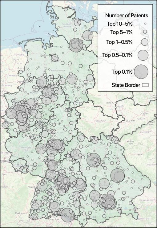
1 Introduction
Innovation has long been emphasized as a key driver of economic growth (Solow, 1957, Romer,
1990). In this process, firms serve as the cradle of most groundbreaking new technologies and
products. For firms, research and development (R&D) serves as an instrument to expand in size
and to increase productivity (Balasubramanian and Sivadasan, 2011), assimilate knowledge from
competitors (Aghion and Jaravel, 2015), and secure long-term growth (Kogan et al., 2017). However,
from a societal perspective, private investments in R&D are generally considered to be below the
social optimum (Jones and Williams, 1998). This is due to positive knowledge spillovers, which make
it difficult for firms to monetize the benefits of new ideas in full (Bloom et al., 2013).
     Against this backdrop, many countries across the world have implemented targeted tax policy
instruments, such as R&D tax credits or extended deduction possibilities for R&D expenses, to spur
firm-level R&D. These policy instruments reduce the burden of business taxes for specific firms
conditional on engaging in R&D. A recent body of research, discussed in more detail below, shows
that targeted R&D tax incentives work, i.e., notably increase firms’ innovative activities. Compared to
this consistent finding, there is very little systematic empirical evidence on the potential disincentive
effects of general business taxes on firms’ R&D activities. This lack of evidence is problematic for at
least three reasons. First, unlike targeted R&D tax incentives, business taxes are in place in almost
every country across the world. Second, knowledge about the size of possible disincentive effects is
needed to optimally design targeted tax incentives for R&D. Third and related, while targeted tax
incentives typically apply to specific types of R&D-active firms only, general business taxes affect
all firms. Knowledge about possible effect heterogeneity across the distribution of (research-active)
firms can be used to improve the accuracy and precision of targeted R&D policies.
     In this paper, we aim to fill this gap by analyzing the impact of profit taxation on plant-level
R&D spending and innovation output.1 We contribute to the small literature studying the effect
of general business taxes on R&D activities by exploiting the unique institutional setting of profit
taxation in Germany, where municipalities autonomously set their local business tax (LBT) each
year. Exploiting around 7,300 local tax changes over the period from 1987–2013, we draw upon
detailed, geocoded biennial panel data that approximately covers the universe of R&D-active plants
in Germany. The dataset, which forms the key basis for Germany’s official R&D reporting to
EU authorities and the OECD, allows us decomposing plants’ overall R&D spending along various
margins, e.g., by distinguishing expenses on internally- vs. externally-conducted R&D projects and
testing for heterogeneous treatment effects along plant characteristics (liquidity and size in particular).
To test for potential accompanying effects on innovation output, we further enrich the data with
administrative information on plants’ patenting activities from the European Patent Office.
     We set up a simple theoretical model that builds upon earlier contributions by Chetty and Saez
(2010) and Chen et al. (2021) to guide our empirical analysis. The model provides three key
hypotheses. First, an increase in the local business tax rate should reduce plants’ R&D investments
because it lowers their after-tax returns. Second, negative effects should be particularly strong

 1   Our empirical analysis is at the level of the plant. We explicitly test for differences between single- and multi-plant
     firms. Throughout the paper, we use the term “firm” in general contexts, i.e., when we refer to mechanisms discussed
     in the literature or institutional features that apply to the firm rather than the plant.

                                                              1
for types of R&D expenditures that are less costly to adjust at the margin. Third, an increase in
the local business tax rate is expected to cause stronger reductions in R&D spending among more
credit-constrained firms. This latter hypothesis draws upon the institutional feature that the costs of
debt financing can be deducted from a plant’s tax base, its operating profits, whereas the costs of
equity financing cannot. This distinct tax treatment distorts plants’ financing decisions towards debt.
However, investments in R&D are generally highly uncertain and come with substantial information
asymmetries between the innovator and financial backers. Moreover, unfinished R&D projects
have little residual value and often lack collateral (Hall, 2002, Brown et al., 2009, Hall and Lerner,
2010, Bakker, 2013)—factors that may make access to debt prohibitively expensive. We thus expect
credit-constrained plants to respond particularly strongly to a given tax increase.
     Our empirical results are in line with theoretical priors. Based on an event study model with
staggered treatment that flexibly controls for varying regional trends, local business cycles, and
political conditions, we show that an increase in the local business tax rate has a negative and
statistically significant effect on plants’ total R&D expenditures.2 We derive a long-term elasticity
of R&D expenditures with respect to the business tax rate of −1.25. This effect size is comparable
with estimates reported in the context of targeted R&D tax credits or subsidies in other settings
(see below for details). We further show that the negative R&D expenditure response is entirely
driven by reductions in internal R&D spending, while the scale of outsourced R&D activities remains
unaffected. We argue that this finding is consistent with steeper marginal adjustment costs for
external R&D spending, e.g., through longer-term partnerships and contracts that are more costly to
alter at the margin. Third, we find that reductions in R&D spending are indeed particularly strong
among credit-constrained plants—as approximated by plants’ age and their non-current liabilities to
sales ratio. In contrast, we do not observe heterogeneity by firm size (employees and sales).
     In a second step, we show that tax-induced reductions in R&D expenditures are accompanied by
lower innovation output—both in terms of raw patent application numbers and when accounting for
quality-differences in innovations by weighting each patent according to the number of citations it
received. The effect materializes with a temporal lag of around two years after the initial tax-induced
decline in R&D spending. The corresponding long-term elasticity with respect to the tax rate is −0.9,
an estimate close to the findings of Akcigit et al. (2021). We further find very similar effects for single-
and multi-plant firms, which indicates that higher business taxes have real negative effects on plants’
innovation output and not only cause tax avoidance behavior of multi-plant firms; e.g., through the
transfer of intangible assets to low-tax countries (see, e.g., Dischinger and Riedel, 2011, Karkinsky
and Riedel, 2012, Griffith et al., 2014, for corresponding evidence).
     Our findings are robust to different specifications of the event study model. In our preferred
specification, we regress plant-level outcome variables on leads and lags of local business tax increases
while controlling for plant fixed effects, sector-by-year fixed effects, federal state-by year as well as
finely-grained commuting zone-by-year fixed effects. Post-treatment effects are stable and robust
to the inclusion of varying regional trends. Pre-trends and additional robustness checks do not
point to the presence of reverse causality or unobserved confounding effects. We also show that
varying local economic conditions, population movements or government expenditures coinciding

 2   Throughout the paper, we focus on tax increases because less than 10% of all tax changes are decreases (see Section 2).

                                                              2
with a given change in the tax rate do not drive our results (see Fuest et al., 2018, for corresponding
earlier evidence). Moreover, our findings remain unchanged when explicitly accounting for possible
heterogeneous treatment effects across cohorts by applying the estimators of Sun and Abraham
(2020) and Borusyak et al. (2021).
     We take our estimates to assess the efficiency of general business taxes to affect firm-level innovation
in comparison with targeted R&D tax policies. Our estimates imply that R&D expenses decrease by
around 0.34 EUR for a tax increase worth 1 EUR in business tax revenues. Equivalent measures of
targeted R&D tax incentives for the UK are much higher—between 1 to 1.7 GBP of increased R&D
spending for each pound decrease in revenues (Dechezleprêtre et al., 2016, Guceri and Liu, 2019).
Thus, targeted tax incentives for R&D expenditures appear to be the more efficient policy instrument
altogether. However, our results question policy makers’ common practice to link firms’ eligibility
for targeted R&D tax incentives to their size. Smaller plants do not react stronger to an increase in
the LBT. Galaasen and Irarrazabal (2021) rather show that size-based eligibility thresholds for R&D
tax incentive may even hinder aggregate economic growth: by promoting the R&D activities of small
firms, size-dependent R&D tax incentives may boost the expansion of relatively unproductive firms
and thus mitigate firm selection.
     Last, we use our empirical set-up to carefully assess the role of innovation for economic growth
and the importance of tax policy in this relationship. In line with the results by Kogan et al. (2017),
we provide suggestive evidence that local innovation has a positive and lasting effect on municipal
economic growth. In contrast, an increase in the local business tax considerably reduces local GDP.
Combining these two pieces of evidence with the estimated plant-level elasticity of innovation output
with respect to the LBT, these findings imply that around eight percent of the total negative effect
of profit taxation on local growth are due to tax-induced reductions in innovation.3 We take these
results as additional evidence for the important role of innovation for economic growth.

Related Literature. Our results contribute to various strands of the literature. We first add to
the small and recent literature that exploits variation in sub-national tax policy settings to study
the effect of (corporate) taxation on innovation. Moretti and Wilson (2017) provide evidence on
the geographic mobility of “star scientists” in response to tax policy changes at the level of the
U.S. states. They find that star inventors are quite responsive to tax incentives, with long-run mobility
elasticities amounting to around 1.8 (−1.7) for personal and corporate income taxes (tax credits).
Akcigit et al. (2021) use U.S. state-level panel data on corporate and personal income tax rates as
well as on patents over the entire 20th century to study the effect of tax policy on innovation. They
find that higher taxes reduce the quantity and quality of innovations and affect the geographic
spread of innovative activities. Moreover, they find corporate inventors to react more to changes
in taxes than individual inventors. Exploiting the same variation in U.S. state-level tax rates over a
shorter time period, Mukherjee et al. (2017) offer similar evidence in showing that increases of the
corporate tax rate reduce firms’ R&D investments and patenting. We contribute to these studies in
two important dimensions. First, we make use of official survey data that approximately covers the

 3   The local business tax can affect growth through other channels than innovation, e.g., by reducing non-R&D investments,
     triggering the re-location of businesses, or lowering wages (Fuest et al., 2018).

                                                              3
universe of R&D-active plants in Germany, which enables us studying detailed plant-level responses
to changes in the local business tax rates. The rich data allows drawing important insights on the
underlying mechanisms, e.g., by differentiating between internal vs. external R&D spending. Second,
the German institutional set-up of profit taxation offers ample variation in tax rates with thousands
of tax changes of substantial sizes. In addition, the local nature of the tax rate variation allows
accounting for possible regional shocks at very fine geographical levels.
  The paper further speaks to the recent literature that analyzes the effects of targeted R&D tax
credits, deduction possibilities, and subsidies. Dechezleprêtre et al. (2016) and Guceri and Liu
(2019) exploit a 2008 reform in the UK’s corporate tax scheme that increased R&D-related deduction
possibilities for medium-sized firms relative to larger ones and document large and positive effects
on R&D spending. Agrawal et al. (2020) exploit a 2004 reform of the Canadian R&D tax credit scheme
for very small firms and also find substantial positive effects. Chen et al. (2021) show that a Chinese
tax policy that awarded corporate income tax cuts to firms with R&D investments over a certain
threshold stimulated R&D activity. Bronzini and Iachini (2014) evaluate a 2003 reform in Northern
Italy, which introduced R&D subsidies for certain industrial research projects. They find that small
firms significantly increased their R&D investments in response to the subsidy, whereas larger firms
remained unresponsive. All studies provide clean causal evidence by exploiting policy cut-offs to
establish quasi-experimental research designs. At the same time, the estimates are clearly local in
nature, referring to firms around the respective thresholds. The data and identification strategy in
our paper allows estimating treatment effects along the full distribution of R&D-active plants. Hence,
we are able to identify average effects but also to test for heterogeneous responses along various
plant characteristics. We can further rule-out mis-reporting effects as documented in Chen et al.
(2021), given that our policy instrument, the LBT, does not specifically target plants’ R&D spending.
  Finally, we connect to a large literature that is concerned with market failures reducing private
R&D activities below socially desirable levels. R&D embodies characteristics of a public good
(Nelson, 1959, Arrow, 1962), such that the social rate of return to innovation is generally well above
the private return (Griliches, 1992, Jones and Williams, 1998). At the same time, expected knowledge
spillovers as well as uncertainty about marketability may lead to private under-investments into
R&D (Czarnitzki and Toole, 2011). Taxes on firms may further lower these private returns, while
social returns remain unaffected. This, in turn, widens the gap between actual and socially desired
levels of R&D in an economy (Klenow and Rodriguez-Clare, 2005).

The remainder of the paper is structured as follows. Section 2 describes the institutional background
of German profit taxation, documents the policy variation we exploit for identification, and briefly
theoretically discusses how an increase in the (local) business tax rate may affect firms’ R&D
investments. Section 3 describes the plant-level dataset, as well as the matching of patent information
and additional financial variables to the set of covered plants. In Section 4, we set up our empirical
research design and test the plausibility of the design’s underlying identifying assumptions. Section 5
presents the corresponding estimates on plant-level R&D expenditures and innovation output.
Section 6 discusses the implications of our results for tax policy and regional economic growth.
Section 7 concludes.

                                                  4
2 Profit Taxation and R&D Incentives
2.1 The German Local Business Tax
Business profits are taxed along two different margins in Germany. At the national level, profits
are either subject to the corporate or personal income tax depending upon a firm’s legal status. In
addition, both corporate and non-corporate firms are subject to the local business tax (Gewerbesteuer),
which is levied at the municipality level.4 Our analysis will exploit within-municipality variation in
local business tax rates for identification.
The local business tax (LBT) is the most important source of revenue for German municipalities
The tax base is operating profits, with limited loss carryforward and no loss carryback. Importantly,
and unlike the tax rate, rules for the tax base are defined at the national level and cannot be altered
by state or municipal governments. The tax rate is derived as the product of the basic federal tax rate
(Steuermesszahl) and a local scaling factor (Hebesatz), which acts as a municipality-specific multiplier:
Local Business Tax Rate τ = Basic Federal Tax Rate × Municipal Scaling Factor.
This scaling factor serves as municipalities’ margin of adjustment. At the end of each year, municipal
councils autonomously decide whether and how to adjust the scaling factor for the upcoming year.
In contrast, the basic federal tax rate is set by the national government and uniformly applies to all
municipalities.5
Figure 1 illustrates the spatial and temporal variation in local tax rates across West Germany.6
Panel A plots, as an example, the 1995 LBT rates for each municipality. We observe substan-
tial differences across the country, with tax rates varying between zero and 45 percent (first per-
centile: 12.5%; 99th percentile: 22.5%). In addition, we see that tax rates are spatially correlated
at the level of the federal states. This can be reconciled with varying fiscal equalization schemes
across states, a feature we account for by including state × year fixed effects in the estimations (see
Section 4.1 for details). Panel B highlights the variation in LBT rates within municipalities over time.
On average, municipal councils decided to alter their local business tax rate three to four times
between 1987 and 2013—the first and last year of tax data used in the analysis.7 Thus, the average
municipality changed its local business tax rate every eight years, which makes changes in the LBT
rather rare events. Around six percent of all West German municipalities did not adjust their scaling
factor during this time span at all.
Figure 2 provides additional information about the underlying variation in tax changes over time.
Panel A shows that more than 90% of all tax changes during the covered period were tax increases;
the majority of them being rather small. The average tax increase amounted to around one percentage
point, or five percent relative to the mean. Notably, the distribution of tax changes is very similar
4 Most firms from the agricultural sector, non-profit organizations as well as self-employed individuals in liberal
professions (such as accountants, journalists or architects) are exempt from this tax.
5 The basic federal rate was 5.0% until 2007. It was reduced to 3.5% in the course of the 2008 German business tax reform.
6 We focus on West Germany because many municipal borders were redrawn in East Germany during the 1990s and
2000s, which prevents the assignment of the exact LBT rate to affected firms. Note that East German plants account for
less than five percent of the country’s total R&D expenditures during the period under investigation.
7 We focus on outcomes from 1995 to 2007 and estimate a dynamic event study specification with a lag of eight and a
lead of six years in our baseline specification (see Section 4.1 for details)
5Figure 1: Spatial and Temporal Variation in Local Business Tax Rates
A. The Local Business Tax Rate in 1995 (in %) B. Number of Tax Changes (1987–2013)
Notes: This figure illustrates the spatial and temporal variation in the local business tax rate across West German
municipalities. In Panel A, the 1995 local business tax rate is plotted for each municipality. Darker colors indicate higher
levels of the LBT. In Panel B, the number of total LBT changes over the period 1987–2013 is plotted for each municipality.
Darker colors indicate a larger number of tax changes in a given municipality. Thick white lines indicate federal state
borders. Maps: © GeoBasis-DE / BKG 2015.
irrespective of how often municipalities altered their LBT throughout the observation period in
total. This implies that there is meaningful variation in long-run tax policies across municipalities,
too. Panel B corroborates this argument. It shows that the long-term evolution of tax rates varied
substantially across West German municipalities, and points to a positive link between the number
of tax increases and the overall change in tax rates over the time period covered in the analysis.
The institutional features of the LBT allow us to base identification on a large number of very local
tax changes while flexibly controlling for common shocks at the federal state and commuting zone
level (see Section 4.1 for details on the empirical strategy pursued).8 In addition, and in contrast to
most other OECD countries, Germany offered no direct or indirect tax incentives for firms’ R&D
spending during the sample period (in fact until January 1, 2020). This makes the country an ideal
laboratory for the research question of interest because no other tax policies need to be accounted for.
Despite this institutional feature, Germany ranks among the world’s most innovative countries (see,
e.g., the annual Bloomberg Innovation Index). During the period from 1995 to 2007, the country’s
8 States and commuting zones are not perfectly nested.
6Figure 2: Variation in LBT Scaling Factors – All West German Municipalities
A. Distribution of Annual Scaling Factor Changes B. Tax Changes over the Sample Period
70
5
60
Share of All Tax Increases (in %)
Number of Tax Increases 1987–2013
4
50
40
3
30
20 2
10
1
0
-50 -40 -30 -20 -10 0 10 20 30 40 50
Annual Relative Change in the Local Scaling Factor (in %) 0
-10 0 10 20 30 40 50 60
Total Increases 1987–2013: 1 2 3 ≥4
Relative Change in the Local Scaling Factor 1987–2013 (in %)
Notes: This graph illustrates the variation in the local business tax rate changes across all West German municipalities.
Panel A illustrates the distribution of annual scaling factor changes for municipalities with varying numbers of total tax
changes throughout the effect window (1987–2013). Panel B illustrates the municipality-level relationship between the total
change in the LBT rate and the number of tax changes throughout the period 1987–2013.
total R&D expenditures amounted to around 2.35% of its GDP on average, which is close to the
U.S. level of 2.54% and much higher than the EU-28 average of 1.65%.9
2.2 Modeling Business Tax Incentives and R&D Investments
In this section, we set up a simple theoretical model of a plant to generate testable predictions about
the impact of business taxation on firms’ innovative activities and its underlying channels. To this
end, we employ a two-period model of a plant that decides on the optimal level of R&D investments
in the spirit of Chetty and Saez (2010). Our model refers to a single-plant firm in a given municipality.
We suppress plant and location indices to simplify notation.
In period one, the plant decides on the level of investment I. The plant uses financial resources P
to finance investments. We start by assuming that the plant collects cash by raising debt D, P = D.
Investment decisions are made in period one, but yield a return of R( I ) in period two, where R is an
increasing and concave function of initial R&D investments (R0 > 0, R00 < 0). To simplify the model,
we abstract from corporate risk-taking. The plant is subject to a profit tax in period two with a tax
rate of τ. We abstract from taxation in the initial period and from policy uncertainty.
Investments generate costs in both periods. In period one, the plant has to pay per-unit investment
cost c. Following Chen et al. (2021), the plant further faces convex adjustment costs g( I ), with g0 > 0,
g00 > 0, when altering the level of R&D investments. Under pure debt financing, the budget constraint
in period one is thus given by P = D = cI + g( I ). In period two, debt D has to be repaid including
9 Own calculations based on the OECD’s Main Science and Technology Indicators database.
7interest r D . Abstracting from discounting, the plant’s profits over the two periods are given by:
π = D − cI − g( I ) + (1 − τ )( R( I ) − r D D ) − D (1)
| {z } | {z }
= π1 = π2
Using the budget constraint from period one, we can rewrite Equation (1) to derive the plant’s
maximization problem:
max (1 − τ )( R( I ) − r D D ) − D
I
s.t. cI + g( I ) = D.
The corresponding first-order condition balances marginal revenues and costs after taxes and
implicitly defines the optimal level of R&D investments I ∗ :
(1 − τ ) R0 ( I ∗ ) = (1 + (1 − τ )r D )(c + g0 ( I ∗ )) if P = D. (2)
Totally differentiating and rearranging terms yields the following comparative-static effect:
dI ∗ R0 ( I ∗ ) − r D (c + g0 ( I ∗ ))
= < 0. (3)
dτ P= D (1 − τ ) R00 ( I ∗ ) − (1 + (1 − τ )r D ) g00 ( I ∗ )
From Equation (3), we derive the following first hypothesis.
Hypothesis 1 (Investment Effect). An increase in the local business tax rate τ lowers the after-tax return on
investments and leads to lower plant-level R&D investments I ∗ .
Hypothesis 1 covers the main empirical test we conduct in this paper. Note that we abstract
from corporate risk-taking in this simple model. Accounting for endogenous risk taking of plants
would yield an additional negative effect on R&D expenses because investments in research and
development are usually of high-risk nature and there is only limited loss offset in the German local
business tax (Langenmayr and Lester, 2018).
Next, we investigate the role of adjustment costs. Verify that dI ∗ /dτ increases in g00 ( I ∗ ). In other
words, the larger g00 ( I ∗ ), the weaker the negative effect of an increase of τ on investment. A simple
example for such an adjustment cost function would be the quadratic function g( I ) = bx2 with
scaling parameters b > 0; see, e.g., Chen et al. (2021) for a similar specification. For very large g00 ( I ∗ )
the investment effect converges to zero. Consequently, we derive our second hypothesis as follows.
Hypothesis 2 (Adjustment Costs Effect). An increase in the local business tax rate τ leads to relatively
smaller reductions in plant-level R&D investments, the stronger the marginal adjustment costs increase in the
level of I, i.e., for investments where g00 ( I ) is relatively high.
Below, we will test this hypothesis by analyzing the effect of a tax increase on internal versus
external R&D investments. Assuming the marginal returns for both types of investments to be
identical in equilibrium, we expect that an increase in local business taxes leads to more pronounced
reductions in internal than external R&D spending because of steeper marginal adjustment costs for
8the latter investment type. By subcontracting R&D to external corporations or entrepreneurs, plants
generally commit to longer-term partnerships and contractual arrangements, which should limit
plants’ ability to alter its marginal external R&D expenditures to a large extent in response to an
increase in the local business tax.
Up to this point, we assumed that the plant finances its R&D expenses in period one by raising
debt. In the context of R&D, credit constraints may be particularly relevant for plants. R&D
investments are generally highly uncertain in their returns and come with substantial information
asymmetries between the innovator and financial backers. Moreover, unfinished R&D projects have
little residual value and often lack collateral (Hall, 2002, Brown et al., 2009, Hall and Lerner, 2010,
Bakker, 2013)—factors that may make access to debt prohibitively expansive for some plants.
Hence, we also explore the effect of taxes on R&D investments when the plant relies upon equity
financing, the alternative financing channel. Abstracting from adjustment costs, the maximization
problem under pure equity financing (P = E) is given by:
max (1 − τ ) R( I ) − (1 + r E ) E (4)
I
s.t. cI = E.
The maximization problem reflects the institutional fact that the costs of equity financing cannot be
deducted from the tax base, which is true for the German LBT as well as in many other corporate tax
systems across the world. The corresponding first-order condition is given by:
(1 − τ ) R 0 ( I ∗ ) = c (1 + r E ) if P = E. (5)
Totally differentiating and rearranging yields:
dI ∗ R0 ( I ∗ )
= < 0. (6)
dτ P= E (1 − τ ) R00 ( I ∗ )
Recall from Equation (3) that the corresponding effect under debt financing is given by:
dI ∗ R0 ( I ∗ ) − cr D
= < 0.
dτ P= D (1 − τ ) R00 ( I ∗ )
With c > 0 and 0 < r D < 1, it holds true that dI ∗ /dτ | P=E < dI ∗ /dτ | P= D < 0. Based on this result,
we derive our final hypothesis.
Hypothesis 3 (Financing Effect). An increase in the local business tax rate τ leads to relatively stronger
reductions in R&D investments for plants that have to finance marginal R&D projects to a larger extent via
equity, for instance, when more binding credit constraints limit debt financing.
Empirically, we test Hypothesis 3 by analyzing whether the negative effect of local business taxes
on R&D investments is different for plants that are more credit constrained and therefore limited in
their capacity to finance investment via debt.
93 Data
Plant-Level R&D Data. Our main data source is the biennial longitudinal dataset Survey on Research
and Development of the German Business Enterprise Sector (henceforth: R&D Survey), collected and
administrated by the Stifterverband on behalf of the German Federal Ministry of Education and
Research. The survey targets all German plants engaged in R&D, and forms the key basis for the
country’s official reporting on its entrepreneurial R&D activities to EU authorities and the OECD.10
The survey contains detailed information on plants’ overall R&D spending, their R&D expenses by
subcategories (internally- vs. externally-conducted R&D, personnel vs. non-personnel R&D spending)
and their R&D staff. Moreover, it offers information on plant size, industry classification, and plants’
organizational structure. Detailed information on each plant’s location of residence further allows
the exact assignment of the applicable LBT in each year.
Our estimation window spans the period from 1995, the earliest year of the survey, to 2007. We do
not cover years beyond 2007 for two reasons. First, we bypass potential R&D effects due to the Great
Recession in 2008–2009. Second, a major tax reform in 2008 altered institutional features of the LBT,
lowering the basic federal tax rate from 5.0 to 3.5 percent and broadening the tax base. Besides
this restriction, we constrain our baseline sample along two additional margins. First, we discard
649 plants (6% of the total sample) that report R&D activities not only for their own plant but for
the entire firm (at different locations). By applying this restriction, we make sure to compare local
changes in the LBT to responses of local plants only. Second, we drop 283 plants which moved during
the survey period to exclude variation that is due to potentially endogenous mobility decisions.11
Ultimately, our baseline sample contains 31,648 plant-year observations in 2,442 municipalities. In
total, these plants spent around 37 billion EUR per year on R&D, which accounts for three-quarters
of Germany’s total R&D expenditures during this period. In Panel A of Figure 3, we illustrate the
spatial distribution of R&D-active plants across municipalities in 2007. We find R&D activity to be
widespread across the country: around one-fourth of all municipalities have at least one R&D active
plant. However, there are also regional clusters of R&D activity; in particular, in south-western
Germany and along the rivers Rhine and Ruhr.
In the baseline estimation sample, plants’ annual total spending on R&D varies from around
EUR 46,000 (5th percentile) to around EUR 16 million (95th percentile); see Panel A of Appendix
Table B.1 for detailed descriptive statistics. The R&D Survey further allows the disaggregation of
plants’ total R&D expenses along two margins. First, information on plants’ expenses for internally-
vs. externally-conducted R&D projects is given. External R&D is typically used as a strategy to
acquire missing knowledge, either by engaging in licensing and outsourcing or starting strategic
alliances. Whereas outsourcing allows firms to exploit economies of specialization and scale, strategic
cooperation generally aims at the development of new technological capabilities (Bönte, 2003, Lokshin
10 The survey also acts as one source of the OECD’s Analytical Business Enterprise Research and Development database
(ANBERD), which has been used in related research (see, e.g., Bloom et al., 2002). See Appendix A for more detailed
information on this dataset.
11 We find very similar effects when including these 283 plants and assigning them the corresponding tax rates prevalent
in their first observed municipality of residence (see below). Moreover, we find no evidence for selective location
choice with respect to the LBT: almost half of those plants that change their location of residence actually relocate to
municipalities with higher local business tax rates.
10Figure 3: Spatial Distribution of R&D Firms and Patenting in West Germany
A. Distribution of R&D Plants B. Distribution of Patents
Notes: Panel A illustrates the distribution of plants in the R&D Survey as of 2007 across West German municipalities. Larger
circles indicate more R&D active plants in a given municipality. Panel B plots the spatial distribution of patenting across
West Germany. Larger circles indicate that more patents were filed in a given municipality throughout our observation
period from 1995–2007. Thick gray lines indicate federal state borders. Maps: © GeoBasis-DE / BKG 2015 and OpenStreetMap
contributors.
et al., 2008). However, the search for and coordination of external contractors and collaborations
also comes with sizable (transaction) costs that may prevent some firms from engaging in external
R&D activities (Berchicci, 2013). In our baseline sample, we observe that half of the covered plants
outsource parts of their R&D activity at least once during the sampling period (see Appendix
Table B.1). On average, external R&D accounts for around 9% of plants’ total R&D expenditures,
and 20% if we consider plants with non-zero external spending only. In addition, we are also able to
distinguish internal R&D spending on personnel from non-personnel expenses (i.e., for materials
and larger investments). On average, two-thirds of plants’ internal expenses accrue to its scientific
staff, who account for around 7% of plants’ total workforce.
Plant-Level Patent Data. To measure innovation output, we link administrative information
from the European Patent Office (EPO) on plants’ patenting activities to the R&D Survey data (see
Appendix A for a detailed description of the matching procedure). Between 1995 and 2007, the
surveyed plants filed 151,862 patents, which accounts for around 60% of all patents filed by German
11applicants at the EPO during this period.12 Panel B of Figure 3 shows the spatial distribution of
patent activity. Overall, the pattern is in line with the regional prevalence of R&D plants. One quarter
of all plants in the R&D Survey filed at least one patent during our sampling period.
The simple count of plants’ number of filed patents may only imperfectly capture the true value
of innovation output if patent quality varies (Scherer, 1965, Hall et al., 2005). To capture varying
patent quality, we construct a second measure of plant-level innovation that weights each patent
by the number of citations it receives from patents filed at the United States Patent and Trademark
Office (USPTO) within five years of its first registration. Previous evidence has shown that such
citation-weighted measures of patent counts correlate well with firms’ private returns to innovation
(e.g., Harhoff et al., 2003, Kogan et al., 2017, Moser et al., 2018).
Following Danzer et al. (2020), we further use detailed textual information from the patent
application files to distinguish product from process innovations. Product innovations generally
relate to new or substantially-altered products that may lead to high social returns. However, these
innovations can be easily appropriated by rivaling firms and face high market uncertainty, which
renders private returns uncertain (Hellmann and Perotti, 2011). In contrast, process innovations, i.e.,
improvements of a given production process, are commonly considered as the more incremental ones
that yield lower social returns but also bear lower risk (Klepper, 1996). We will test below whether
an increase in tax rates affects both types of innovations differently.
Panel B of Appendix Table B.1 provides the corresponding descriptive statistics on plants’ patenting
activities. The average plant files 0.84 patents per year, which receives 1.7 citations over the following
five years. Around 60% of all patents in our sample can be categorized as product innovations.
Financial Information. Whereas the R&D Survey offers detailed information on plants’ R&D
activities, little information is given on plants’ financial situation. However, as hypothesized in
Section 2.2, we expect credit-constrained plants to react stronger to a given tax increase because the
costs of debt financing can be deducted from the tax base while those of equity financing cannot. To
proxy plants’ financial situation, we therefore add information from Bureau van Dijk’s Amadeus and
Orbis databases to the plant-level survey (in particular, information on plants’ age and non-current
liabilities). The two datasets offer a variety of financial information at the firm level, i.e., we assign
the firm-level financial information to plants that are part of a multi-plant firm. As these datasets
predominantly cover larger and oftentimes stock-listed plants, we can only supplement around 40%
of the surveyed R&D plants with additional information from this data source.
Administrative Regional Data. Last, we complement the plant-level data with annual data on local
business tax rates as well as other regional, i.e., municipality- and county-level information. This
includes data on municipalities’ annual public expenditures, population figures, unemployment rate,
and county-level GDP. We will use these variables to test whether local business cycles simultaneously
determine municipalities’ tax setting and plant activities. Panel C of Appendix Table B.1 provides
12 By definition, we do not capture patents filed by the government, public universities, or individual inventors. Moreover,
not all plants that file a patent during the observation period are covered in the R&D Survey and our baseline sample,
respectively. This is especially true for plants with very little or infrequent patent activity.
12the corresponding descriptive statistics. We see that innovation predominantly occurs in urban,
industrialized regions with relatively little unemployment.
4 Empirical Strategy
To estimate the causal effect of changes in the LBT on plant-level R&D expenses and innovation, we
exploit all available changes in the tax rate within a municipality over time in a dynamic generalized
difference-in-differences framework with staggered treatment (Suárez Serrato and Zidar, 2016, Fuest
et al., 2018, Akcigit et al., 2021). In Section 4.1, we describe the empirical implementation. We discuss
the identification of causal effects in our model in Section 4.2.
4.1 Event Study Design
We base our analysis on an event study setup that treats each tax change as an independent event.
This allows us to exploit all available variation in local tax rates within municipalities over time. More
precisely, we regress a given outcome Yit of plant i in year t belonging to sector s (manufacturing,
services, and other) located in a municipality m and commuting zone z on leads and lags of the
k . Treatment is either defined as an indicator for a tax change, or a tax change
treatment variable Tmt
dummy interacted with the size of the change (see below for more details). The corresponding
regression model is given by:
Yit = ∑ βk Tmt
k
+ µi + θzt + ζ st + ε it . (7)
k
We transform outcomes—R&D spending, the number of patents, and various subcategories of the
two—using the inverse hyperbolic sine (IHS) transformation.13 Plant fixed effects (µi ) account for
unobserved time-invariant confounders at the plant level.14 Moreover, state × year and commuting
zone × year fixed effects, both included in term θzt , as well sector × year fixed effects, ζ st , control for
regional and sectoral time-varying confounders, respectively. We calculate cluster-robust standard
errors that account for potential correlations across plants, years, and sectors within municipalities.
We adjust this generic event study outline in three dimension to fit our empirical setting. First,
we account for the biennial structure of the R&D Survey and base our analysis on the subset of
odd years t = 1995, 1997, . . . , 2007 to harmonize samples across outcomes. Leads and lags of the
k , thus sum tax changes in two consecutive years to account for tax reforms in
treatment variable, Tmt
even-numbered years as well. In our preferred specification, we restrict the effect window to six years
before and eights year after a tax reform, i.e., three leads and four lags in the given two-year structure
of the data, k ∈ [−6, −4, . . . , 8]. Moreover, we normalize the last pre-treatment coefficient, β −2 , to
zero, i.e., all effects are relative to two years before treatment.
13
p
For any outcome ỹ, the inverse hyperbolic sine transformation is defined as: y = ln(ỹ + ỹ2 + 1). This transformation
comes with the advantage of being well-defined for zero values. This is particularly relevant for the plant-level patent
outcomes in the context of this study. For larger values, the IHS transformation is almost identical to the canonical log
transformation. We show below that the transformation of outcome variables does not drive the estimates.
14 We exclude plants that move throughout the observation period in our baseline specification. When adding these plants
in robustness checks, we add municpality fixed effects ( λm ) to the regression model.
13Second, we account for multiple tax changes per municipality by binning the endpoints of the effect
−6 8 ,
window (McCrary, 2007). Hence, the first lead of the treatment variable, Tmt , and the last lag, Tmt
take into account all tax reforms that will happen six or more years into the future from period t
onward or happened eight or more years in the past, respectively. The underlying assumption is
that (pre)-treatment effects are constant beyond these endpoints (Schmidheiny and Siegloch, 2020).
Formally, we define the leads and lags of the treatment variable in the following way:
−6
∑ j=−∞ m,t− j
D if k = −6
k
Tmt = Dm,t−k if − 6 < k < 8 (8)
∑∞ D
if k = 8,
j =8 m,t− j
where Dm,t is the actual tax reform indicator denoting treatment in year t.
Third, we use two alternative definitions of treatment. On the one hand, we use a simple dummy
variable specification adjusted to our biennial data. Treatment is the sum of two dummy variables
indicating a tax increase from t − 1 to t and t − 2 to t − 1 (Equation (9a)). On the other hand, we take
into account the full variation in the local business tax rate by scaling the dummy variable with the
size of the tax change (Equation (9b)):
inc
Dm,t = 1(τmt > τm,t−1 ) + 1(τm,t−1 > τm,t−2 ) (9a)
cha
Dm,t = 1(τmt > τm,t−1 ) · (τmt − τm,t−1 ) + 1(τm,t−1 > τm,t−2 ) · (τm,t−1 − τm,t−2 ). (9b)
Implied Elasticities. While event study estimates inform about dynamics of treatment effects, it
is useful to derive one central take-away elasticity. Our baseline summary measure is the elasticity
as implied by the estimates of the last lag in the event study regressions, βb8 , which measures the
long-run effect more than seven years after the tax reform. We compare these implied long-run
elasticities to medium-run elasticities and simple difference-in-differences estimates in Section 5.
4.2 Identification
To estimate causal effects, we relate within-plant changes in R&D activities to changes in LBT rates
while absorbing common, time-varying shocks to federal states, commuting zones, and economic
sectors. To interpret estimates βbk as causal effects, we have to assume that tax changes are not
systematically correlated with (trends in) local factors within the same federal state, commuting
zone, and economic sector that also affect plants’ R&D expenses or innovative activities. Small and
insignificant pre-treatment coefficients in the event study estimates would support this assumption,
as most confounding effects that violate the identifying assumption would show up as diverging
pre-trends. Similarly, if reverse causality was an issue—i.e., if local policy-makers would adjust LBT
rates because of changes in plants’ innovative activities—we should observe diverging trends in
R&D investments before treatment. As shown in Section 5, pre-trends across the different event study
specifications are indeed flat for the set of plant-level outcomes under investigation.
Another concern for identification are confounding shocks that coincide with the tax change,
but have no visible effect before treatment. Whether such shocks are able to impede identification
14depends on the geographical level at which they arise. Our preferred specification includes state-by-
year fixed effects, which control for any change in state policies or varying electoral cycles. To control
for shocks below the state level, we also account for time-varying economic or political shocks at
the level of the 204 West German commuting zones (Arbeitsmarktregionen, henceforth CZ) in our
baseline specification.15 However, to test the sensitivity of our results with respect to the potential
presence of regional shocks at varying geographical levels, we deviate from this baseline model
below and replace the CZ-by-year fixed effects with coarser and finer regional controls, respectively.
If systematic local shocks were to violate our identifying assumption, we would expect results to
differ alongside these changes in the empirical specification. Precisely, we absorb common shocks at
the level of the 28 administrative districts (Regierungsbezirke, NUTS II), the level of the 71 statistical
planning regions (Raumordnungsregionen, ROR), or the 272 counties (Kreise und kreisfreie Städte) in
alternative specifications, respectively. Appendix Figure B.2 illustrates these different jurisdictions
for the federal state of Bavaria. We find hardly any difference in pre-treatment effects when moving
between specifications. Post treatment, treatment effects become somewhat larger (in absolute terms)
when controlling for shocks at finer regional levels.
We also take these findings as evidence in favor of the validity of the stable unit treatment value
assumption (SUTVA) with respect to local innovation spillovers. Recent work by Matray (2021) shows
that these spillovers are generally positive, which would suggest that we might underestimate the
true effect of a tax increase on R&D activity. This potential bias should become larger the finer we
control for regional trends because the respective control group becomes more and more restricted to
municipalities in close proximity to the treated one. The fact that our estimates become even larger
when including finer regional time controls suggests that the SUTVA is not violated.
Finally, economic or political shocks may also occur at the municipality level and, potentially,
coincide with the timing and size of the tax change. In this regard, one might particularly worry
that local economic developments at the municipal level simultaneously determine municipal tax
setting and plant activities. We address this concern twofold. First, we show that socioeconomic
indicators at the municipality level (population, the share of unemployed among the population,
public expenditures, and public revenues) do not display any systematic pre- or post-trend when
used as dependent variables in the event study model as set up in Equation (7); a finding in line
with previous studies (Fuest et al., 2018, Blesse et al., 2019).16 Second, we sacrifice some econometric
rigor and include lagged socioeconomic indicators in our baseline event study model. While these
additional variables may constitute “bad controls”, estimated effect patterns remain unaffected.
Heterogeneous Treatment Effects. Recent contributions by Sun and Abraham (2020), Callaway and
Sant’Anna (2020), de Chaisemartin and D’Haultfœuille (2020), and Borusyak et al. (2021) have shown
that standard two-way fixed effects models with staggered treatment may deliver biased estimates
in case of treatment effect heterogeneity across cohorts, i.e., in case the impact of a given treatment
varies with the year of its implementation. In our setting with multiple treatments per unit over time,
we address this concern by restricting the sample to those municipalities that experienced either no
15 On average, there are eight municipalities and 25 plants per commuting zone in our baseline sample.
16 In Section 6.2, we also investigate the effect of LBT increases on local GDP. Besides establishing flat pre-trends, we show
that local GDP declines in response to a tax rate increase (see Panel A of Figure 8).
15or just one tax increase throughout the observation period. We show that the standard event study
estimates for this sub-sample are close to the ones from our baseline sample. We then apply the
estimators proposed by Sun and Abraham (2020) and Borusyak et al. (2021) to the sub-sample and
show that our results remain unchanged when explicitly accounting for the potential presence of
hetereogeneous treatment effects across cohorts (see Section 5.1 for detailed results).
5 Empirical Results
We next present our empirical results. We first investigate whether an increase in the local business
tax rate reduces plants’ total R&D spending (Hypothesis 1)17 and extensively test the robustness
of our key effect of interest. We then analyze whether the tax-induced reductions are indeed
particularly strong for R&D investment types with flat marginal adjustments (Hypothesis 2) and for
credit-constrained plants (Hypothesis 3). Last, we investigate the corresponding effects of an increase
in the LBT on innovation output as measured by the (citation-weighted) number of filed patents.
5.1 Effects on Overall R&D Spending
Figure 4 presents the estimated dynamic effect of an increase in the local business tax rate on plants’
total R&D spending from the two different event study models as defined in Equations (7)–(9b). First,
we notice that pre-trends are relatively flat and statistically insignificant. In line with Hypothesis 1,
we further detect that an increase in the LBT rate exerts a substantially negative and statistically
significant effect on plants’ total R&D spending post treatment. The effect builds up over the first
two years and levels off thereafter. Effects are similar when using the simple tax increase dummy
variable or the actual size of the tax rate increase as treatment.18 The binary event study model as
given by Equation (9a) will serve as our baseline specification throughout the rest of the paper.
In terms of magnitudes, our long-run estimate ( βb8 ) implies that a one percentage point increase
in the local business tax leads to a decrease in R&D spending of 6–7% after eight years. This
semi-elasticity translates into a long-run elasticity of around −1.25. In Appendix Figure C.2, we
report alternative summary estimates of the effect size and their respective confidence intervals using
different lags of the classic event study model or when estimating a simple difference-in-differences
model with the same set of fixed effects.
We conduct several sensitivity checks to test whether our baseline estimates are robust to varying
specifications of the event study model.
Time-Varying Confounders. Departing from our baseline model with state-by-year and commuting
zone-by-year fixed effects, we first re-estimate the event study model with less or more fine-grained
region-by-year fixed effects (at the NUTS-II, ROR, or county level). Changes in the event study
coefficients are informative about the importance of local shocks as a potential source of bias.
Panel A of Appendix Figure C.3 shows that effects are statistically significant at conventional levels
17 As shown in Appendix Figure C.1, we find no corresponding positive effect of a tax decrease on R&D spending.
However, in light of the relatively few tax decreases in our sample, we shy away from emphasizing this particular result.
18 The average tax rate increase is almost equal to one percentage point (cf. Section 3).
16You can also read