Dynamic graph and polynomial chaos based models for contact tracing data analysis and optimal testing prescription
←
→
Page content transcription
If your browser does not render page correctly, please read the page content below
Dynamic graph and polynomial chaos based models for contact
                                                    tracing data analysis and optimal testing prescription
                                                                       Shashanka Ubaru*              Lior Horesh               Guy Cohen

                                                                                    IBM T.J. Watson Research Center
arXiv:2009.04971v4 [q-bio.PE] 10 Sep 2021

                                                                                      Yorktown Heights, NY, USA

                                                                                                    Abstract
                                                       In this study, we address three important challenges related to disease transmissions such as the
                                                   COVID-19 pandemic, namely, (a) providing an early warning to likely exposed individuals, (b) identifying
                                                   individuals who are asymptomatic, and (c) prescription of optimal testing when testing capacity is limited.
                                                   First, we present a dynamic-graph based SEIR epidemiological model in order to describe the dynamics of
                                                   the disease propagation. Our model considers a dynamic graph/network that accounts for the interactions
                                                   between individuals over time, such as the ones obtained by manual or automated contact tracing, and
                                                   uses a diffusion-reaction mechanism to describe the state dynamics. This dynamic graph model helps
                                                   identify likely exposed/infected individuals to whom we can provide early warnings, even before they
                                                   display any symptoms and/or are asymptomatic. Moreover, when the testing capacity is limited compared
                                                   to the population size, reliable estimation of individual’s health state and disease transmissibility using
                                                   epidemiological models is extremely challenging. Thus, estimation of state uncertainty is paramount for
                                                   both eminent risk assessment, as well as for closing the tracing-testing loop by optimal testing prescription.
                                                   Therefore, we propose the use of arbitrary Polynomial Chaos Expansion, a popular technique used for
                                                   uncertainty quantification, to represent the states, and quantify the uncertainties in the dynamic model.
                                                   This design enables us to assign uncertainty of the state of each individual, and consequently optimize the
                                                   testing as to reduce the overall uncertainty given a constrained testing budget. These tools can also be
                                                   used to optimize vaccine distribution to curb the disease spread when limited vaccines are available. We
                                                   present a few simulation results that illustrate the performance of the proposed framework, and estimate
                                                   the impact of incomplete contact tracing data.

                                            1     Introduction
                                            Contact tracing is considered one of the most effective methods to curb the spread of transmissible diseases
                                            such as COVID-19 [14]. Contact tracing is a process by which the whereabouts and interactions of an infected
                                            individual with other individuals are carefully mapped. The key information that is sought is the physical
                                            proximity between individuals and for how long the individuals interacted. Additional information such as
                                            the environment where the interaction took place (for example, a close room with poor ventilation or an
                                            outdoor space) can also be recorded.
                                                Contact tracing can be manual or digital. Manual contact tracing is usually performed by a contact tracer,
                                            a trained health-care worker, who interviews the infected individual. Based on the infected individual’s
                                            recollection of events, calendar records, credit card records, etc. the contact tracer can build a list of exposed
                                                * Corresponding   author, Shashanka.ubaru@ibm.com

                                                                                                         1
individuals that were in proximity to the infected individual and recommend action such as quarantine or
testing of the exposed individuals. Digital contact tracing augments the work of a contact tracer. Individuals
who participate in digital contact tracing typically carry a device that tracks their proximity to other individuals.
As an example, an individual’s smart phone can be used to periodically transmit a unique identifier and also
record transmissions of identifiers sent by nearby devices. The signal strength of the recorded transmissions
can be used to estimate the proximity to other individuals [56, 17, 21, 46, 41, 5]. Digital contact tracing that
relies on this method was recently implemented by Google and Apple [6] for COVID-19 and is now available
in most iOS and Android based smart phones. Digital contact tracing such as the one provided by Google
and Apple is a crowd-sourcing method and its efficacy depends on adoption by the public. Furthermore, the
method which uses Bluetooth transmission may inaccurately estimate of proximity due to signal attenuation
or reflections from nearby objects. However, in the workplace, on university campuses, and in schools,
contact tracing can be mandated. Active or passive devices like RFID bracelets or badges that are tracked by
indoor sensors, can be used inside organization’s campuses to obtain reliable and accurate digital contact
tracing data. For the purpose of this work we assume that contact tracing data is obtained by any of the
methods discussed above.
Some epidemics/pandemics, including the recent COVID-19 pandemic have proved difficult to contain
due to the large population of asymptomatic individuals. Asymptomatic people are individuals who are
infected with the virus but have no symptoms. Asymptomatic people can be contagious to others. It is
estimated that up to 40% of COVID-19 infected individuals are asymptomatic [36, 37, 62]. Estimating
the asymptomatic individuals is therefore needed to successfully curb the spread of the disease. Testing
and vaccine distributions are the other important areas that have proved to be difficult and have impeded
the efforts to contain the spread of viruses. Without a doubt, testing is likely the most important tool that
health-care professionals have to assess the spread of viruses within the population, yet the lack of testing kits
and lab resources continues to limit testing volume. Additionally the cost of testing may also limit testing in
disadvantaged communities. Since testing is a limited resource, testing the entire population periodically is
not feasible and therefore it is of great importance to optimally prescribe testing. Once effective vaccines
are available, efficient vaccine distributions can curb the disease spread successfully. However, vaccine
availability could be limited, and tools to optimize vaccine distribution under limited vaccination budget are
necessary.
Our contributions: In this paper we employ contact tracing data to infer which individuals are likely to
be asymptomatic and which individuals should be tested to mitigate uncertainty of the overall network. We
prescribe an optimal testing recommendations to mitigate the overall risk under the constraints of limited
testing resources. To achieve these goals we start by representing the contact tracing data as a dynamic graph.
Each node represents an individual, and connections between the nodes represents the interaction between
individuals, such as physical proximity and duration of contact. We use a compartmental epidemiological
model to evolve the graph in time. The evolution also incorporates new data from contact tracing as well as
new testing and vaccination data of individuals.
One of the epidemiological models that has been considered suitable for modeling disease propagation is
the SEIR model (Susceptible, Exposed, Infected, Recovered). This model takes into account an incubation
period during which individuals that have been infected are not yet infectious themselves [31, 32, 33, 18, 7, 12].
We note that our method is not tightly tied to the SEIR model and is applicable to any other models that
describe disease transmission among populations. The SEIR model treats the entire population as a whole and
is unaware of the connections and interaction between individuals. In this work we add graphical dependency
to the SEIR model equations, so the details of how individuals interact impact the model accounting for the
2spread of the disease. The modified SEIR model is now described using a set of partial differential equations,
with a graph Laplacian operator that accounts for the interaction between individuals as captured by the
contact tracing data. Both the contact network and the paramters of the model can be time varying. In another
deviation from the original SEIR model, we treat the S, E, I, R populations as probabilities (similar to
[59, 48, 22]), rather than compartmental populations.
Using the aforementioned model or a similar model, it is possible to provide an early warning to
individuals who are likely to be exposed or infected and also identify those individuals who are likely to be
asymptomatic. The latter have a high probability of being infected while showing no symptoms. The second
challenge that we addressed is how to prescribe optimal testing while both targeting individuals conferring
eminent risk to their surrounding as well as dedicating precious testing allocation towards providing a more
accurate picture of the overall risk by mitigating the overall model uncertainty. Given the large-scale nature
of the problem, we propose here a Polynomial Chaos Expansion (PCE) framework to offer a rapid means for
sampling the posterior distribution of the state. Quantifiable assessment of the uncertainty associated with
each node in the underlying state enables identification of nodes (e.g. nodes of high variance) in the graph in
which point estimate predictions can provide spurious results. It is critical to judiciously assess the degree
of confidence we can attribute to our predictions, and devise means to proactively mitigate uncertainty by
testing, rather than merely settle with its quantification. For this, we propose optimal testing prescription by
solving an optimization problem that accounts for (a) high risk individuals according to the model, (b) the
uncertainty in the model, and (c) the testing budget available. We present simulation results that illustrate
the models’ behavior and show how we can issue early warnings to likely exposed/infected individuals and
prescribe optimal testing to control uncertainty and mitigate the disease spread.
If effective vaccines are available, our graphical SEIR model can account for individuals who are
vaccinated. We can either incorporate another state (say vaccinated V ) or alternatively consolidate vaccinated
with the recovered state, with slow temporal relaxation time (per the diminishing protection that a vaccine
offers). We can partition the graph and isolate communities who are vaccinated, and can ensure that the
individuals who are linking between communities are vaccinated to act as buffers. We can also modify the
objective of the optimization to include vaccination of individuals, taking into account the expected risk
to individual and their connectivity, the uncertainty in their state, and the amount of vaccines available, to
optimize vaccine distribution.
Related work: Since the last year, a plethora of works have been burgeoned in the literature that model
the COVID-19 disease transmission. A number of variants of the SEIR model and other transmission
models have been proposed, such as the SEIR models [60] used to analysis the spread of COVID-19 in
China [45, 54, 15, 37, 52], in Europe [22, 39, 38], in India [11, 49, 27] and in Africa [65]. Several other works
exist too, that model the different aspects of COVID [9, 26, 1, 28, 50, 34, 61] and others. Many machine
learning and AI techniques have also been explored [66, 40, 57, 35].
Network based models have also been studied in the literature for analyzing disease spread [59, 25] and
optimized vaccine allocation [48, 10]. In these papers, a network based ODE model called the N -Intertwined
model is proposed for analyzing the spread/transmission of COVID-19 among population. In [25], the state
of the nodes is assumed to be in one of the predefined compartments, while in [59, 48, 10] the states are
stochastic. The network is assumed to be a static random graph in these models. In [48, 10], a (combinatorial)
optimization problem involving a cost function of the states and constraint on the largest eigenvalue of the
adjacency matrix of the graph is solved to optimize vaccination of the population in the network.
However, to the best of our knowledge, our work is the first to incorporate contact tracing information
into the SEIR model as dynamic graphs and use the graph Laplacian for state evolution, to model the disease
3propagation. This, along with with S, E, I, R states as probabilities, enable us to issue early warnings
to individuals who are likely to be exposed and/or infected (are asymptomatic). We also propose the use
Polynomial Chaos Expansion to quantify uncertainties in the model and the measurements (test results) and
present a method to prescribe optimal testing in order to control these uncertainties and mitigate the spread of
the disease. These challenges have not been addressed in a systematic way in the prior works.
2 Problem formulation
For the sake of simplicity we assume a population of n individuals, yet, representation of varying population
size over time can also be considered. We begin by defining the notation of a probabilistic individualized
pandemic state tensor, its dynamics and the measurement operations.
2.1 State
Let the state of individual i ∈ N at time step t ∈ N be represented by the probability vector yi,t ∈ R4 =
{Si,t , Ei,t , Ii,t , Ri,t }, where Si,t , Ei,t , Ii,t , Ri,t ∈ [0, 1] and the normalization condition applies Si,t + Ei,t +
Ii,t + Ri,t = 1. Thus, we assume that at each time step, an individual carries probabilities of being either
susceptive, exposed, infected or recovered. The proposed framework is not restricted to the aforementioned
choice, and obviously other probabilistic state representations corresponding to alternative pandemic models
can equally be considered. Assuming T times steps has evolved from an initial state, the state of the
dynamic system is represented by the 3rd degree tensor Y ∈ Rn×4×T . Incorporation of a dynamic model
(even mis-specified) offers means for the incorporation of a smooth temporal prior upon the evolution of
these probabilities implicitly. The state can enriched with stationary sites, such as public places, to enable
transmission of disease via surface contact. Yet, proper representation of such sites may require a different
state space representation as well as dedicated dynamics.
2.2 Measurements
Graph data: Let Gt ∈ Rn×n represent weighed graph data attributed to each time step. The graph
represents proximity interaction between individuals. The weights on the edges factors both proximity as
well as exposure duration within a single time step. Such data can be acquired from peer-to-peer short-range
communication on smart devices, such as Bluetooth [17, 8, 6, 5]. Since the interactions between individuals
changes over time, the set of weighted graphs forms a dynamic graph over time. We shall denote the graph
Laplacian of each temporal graph Gt , by Lt ∈ Rn×n , and is given by Lt = Dt − At , where Dt is the
diagonal degree matrix and At is the adjacency graph obtained from the proximity/contact tracing data.
Infection test data: In addition to the graph data, we shall assume that testing for infection are administrated
at each time step. Such tests may include PCR (Polymerase chain reaction), antibody testing such as
Immunoglobulin G (IgG) or Immunoglobulin M (IgM), or any other means to assess the definitive infection
state for tested individuals with measurable confidence level. Specifically, here we are interested in tests that
qualify whether an individual is actively infectious (attributed to the 3rd components of individual’s state at
the timestep the test was collected). The number of such infection indicating tests (IIT) taken at each time
steps may vary and given by mt , whereas the results of the tests are denoted by dt ∈ Rmt , mt < n. For the
sake of data assimilation, we denote a linear projector operator Pdt ∈ Rmt ×n which projects the state at time
step t to the IIT measurement space.
4Recovery test data: Respectively, we shall denote by pt < n the number of recovery indicating tests (RIT)
taken at time step t and by ht ∈ Rpt the tests results. The RIT test qualifies whether an individual has been
recovered. Similarly, as with the IIT tests, we define a linear projector Pht ∈ Rpt ×n that projects the state at
timestep t to the RIT measurement space. If and when effective vaccines are available, individuals who are
vaccinated can be marked as recovered in the model.
Surface test data: Transmission of viral content can be made via stationary surfaces, rather than merely by
face-to-face interaction of individuals [16, 47]. It is possible to incorporate into the pandemic transmission
model tracing data representing interactions between individuals and physical sites (e.g. via interaction with
stationary Bluetooth device or RFID). Positive outcome of the test, will indicate that infectious particles
were identified at a site. These tests can be treated similarly as IIT tests (attributed to the 3rd components of
individual’s state at the time step the test was collected) or otherwise can be handled differently by augmenting
the SEIR model. The number of surface tests taken at each time steps is given by qt , whereas the results of
the tests are denoted by gt ∈ Rqt , qt < n. We denote a linear projector operator Pgt ∈ Rqt ×n which projects
the state at time step t to the surface test space.
Cleaning / disinfecting event data: When physical sites are incorporated into the model, it is essential to
indicate records of cleaning / disinfecting events which effectively reduce / reset the site to a state of having
little probability of being infectious, that is annihilating the 3rd components of individual’s state at the time
step the test was collected. Let the number of such recorded events be denoted by ct < n with respective
recorded values vt ∈ Rct . The linear projector Pvt ∈ Rct ×n that projects the state at time step t to the
disinfecting events.
2.3 Dynamics
To describe the dynamics of the model we modify the conventional SEIR population model, to an individ-
ualized, probabilistic graphical model. While the SEIR model has been employed extensively in disease
control simulation, in the context of this study, other dynamical models can be equally utilized. Provided
the interaction graph data between individuals over time as well as individuals pathogenic testing data, we
shall recast the model as individualized model, where each node represents an individual, rather than address
populations. Interactions between individuals and exchange of probabilities at the tth timestep are represented
using the graph Laplacian Lt ∈ Rn×n . The revised model is a stochastic diffusion-reaction1 model of the
following form:
ds
= −κS Ls − βe s − γi s + µs s (1)
dt
de
= −κE Le + βe s + γi s − αe (2)
dt
di
= −κI Li + αe − µh i − µs s (3)
dt
dr
= µh i (4)
dt
where {s, e, i, r} ∈ Rn are vectors containing the states {S, E, I, R} for all individuals, respectively,
κS , κE , κI ∈ R are diffusion coefficients and α, β, γ, µh , µs ∈ R represent reaction coefficients. The
1
It is important to note that other than the diffusion-reaction model considered here, alternate transport models such as wave
relaxation, etc, can be considered. The discussion of such models goes beyond the scope of this study
5model coefficients can be prescribed a-priori, but, whenever sufficient data is provided, these coefficients
can be learned statistically2 . The coefficients of the model themselves may evolve over time to reflect
changes in individuals behaviour (e.g. masks wearing compliance, hand sanitation frequency, etc). Such
refinements of the model can be accommodated by devising parametric / non-parametric models for the
coefficients themselves, that includes additional health-care policies and public compliance affinity parameters.
Furthermore, structural mis-specification of the dynamical model can be mitigated via hybridization of first-
principle and data-driven model learning [53, 51]. Other then advocating for models that enables probabilistic
treatment of individual state, and the incorporation of graphical data, the scope of this study focuses on
closure of the tracing-sensing loop, rather than the intricacies of any particular model. Thus, for the sake of
expositional simplicity we shall proceed with the above exemplar model.
Integration of the aforementioned continuous-time dynamical system (1) can be performed in various
ways, such as implicit-explicit combination [30], high order Runge-Kutta integrators [13], etc. Given the
frequent rate of the graph data, and the complexity associated with semi-explicit integration schemes, we
shall resort here to a simple forward Euler integration. Obviously, when such explicit integrator is employed
it is essential to ensure stability of the numerical solution via careful selection of timestep duration. Other,
more complex integration schemes can equally be considered. Under these settings we have:
st+1 = st − ∆t·(κS Lt st + βet st + γit st ) (5)
et+1 = et − ∆t· (κE Lt et − βet st − γIt St + αEt ) (6)
it+1 = it − ∆t·(κI Lt it − αet + µit ) (7)
rt+1 = rt + ∆t·µ·it (8)
where ∆t is the time step parameter. Note that the graph Laplacian Lt incorporated in the model is time-
varying, per the dynamic interaction between individuals over time. The contact-tracing data and the contact
network are typically time varying, and it is important that the model accounts of these time dependent
variations. The initial conditions of the model are generally unknown a-priori. In the following section, we
shall discuss how uncertainty associated with these conditions can be quantified and mitigated.
Asymptomatic individuals: The proposed model assumes probabilistic state y = {S, E, I, R} for indi-
viduals, and these probabilities are estimated using the contact tracing data and the model evolution. We
start with an initial state t = t0 , where the individuals who were tested positive will have Ii,t0 = 1 and the
remaining individuals start with Si,t0 = 1. Next, the model is evolved, taking into account the contact tracing
data (via. the dynamic graph Laplacian) to obtain the probability states at a given time t = T . We can then
use these probabilities to (a) issue early warning to individuals who have a high exposed state E at the given
time T , and (b) more importantly, identify those individuals who are asymptomatic to the disease. Such
individuals will have a high infected state I, but might not have any symptoms and hence are likely not tested.
The uncertainty quantification analysis described in the following section can be further used to identify such
individuals (with uncertainty in state estimation) and prescribe testing.
Data Assimilation In order to provide point estimate of the state Y given measurements (testing) up till
t = T , we can consider a dynamic inverse problem that accounts for the IIT and RIT tests and the associated
noise in the models. For example, we can consider the following problem:
2
Diffusion and reaction coefficients may be set a-priori differently to model individuals dynamics, vs. sites.
6Ŷt = arg min R (Yt+1 , ft (Y )) (9)
Y =[s,e,i,r]∈Rn×4
T
X
s.t. ηt ·(δd (Pdt i, dt ) + δr (Pht r, ht ) (10)
t=t0
+δg (Pgt Y , gt ) + δv (Pvt Y , vt )) ≤ τ
where ηt ∈ R represents a discount parameter, representing the degree to which one wish to factor older data
(e.g. rely more heavily on recent data rather than old one), and δd , δr are noise models associated with IIT
and RIT tests respectively. Similarly, δg , δv and R are error metrics, ft is the evolution function that takes the
state Yt to the next time step via. (5)-(8), and Yt+1 is the updated state after including the test results. An
alternative assimilation model would be to enforce the known testing data, rather than consolidate it with
prior knowledge of disease propagation.
Such a point estimator can be useful, yet they do not provide means for estimation of the posterior
probability, and therefore, can be limiting when it comes to uncertainty quantification, and experimental
design. Conventionally, one can sample the prior distribution associated with the state and update the posterior
using methods such as Markov Chain Monte Carlo (MCMC) or Hamiltonian Monte Carlo. Alternatively,
methods such as generalized and arbitrary Polynomial Chaos Expansions can offer more salable means to
sample the posterior in large-scale settings [20, 43, 2].
3 Uncertainty Control
Due to limited testing capacity, in most cases testing is performed sparsely, where the number of tests is
XT XT
significantly smaller compared to the dimensions of the state space mt < n, rendering the state
t=t0 t=t0
inference problem ill-posed. Furthermore, the intrinsic recovery function, the interaction dynamics, and the
measurements are all mis-specified, and therefore admitting uncertainty. Assuming some form of regularity
of the solution (primarily in the form of the dynamical model), we can still make substantiated inferences,
yet, we must consciously account for the underlying uncertainty associated with each inference. Whenever
an observation (testing) takes place, one can attribute relatively high degree of confidence (small uncertainty)
to the probability assigned to the relevant node, yet, the further we traverse away from that node across the
graph, or propagate over time, the level of confidence decays.
Appropriate representation of uncertainty, is critical for making judicious decision as for how to prioritize
best the administration of a limited testing budget. This overarching mission is essence of this study. On
the one hand, it is eminent to test those identified to be under high risk (high probability of being infected),
as such individuals confer immediate risk to their surrounding, yet on the other hand, acknowledging the
limitation of the model, we wish to allocate testing as to reduce the degree of uncertainty associated with
nodes for which uncertainty is high, as we otherwise, favor exploitation over exploration, and may miss the
bigger picture altogether.
3.1 Polynomial Chaos Expansion
Polynomial Chaos Expansion (PCE) is a non-sampling based formalism used for the quantification of
prediction uncertainties in stochastic systems [23, 64, 43]. The key idea is to depart from the traditional point-
7wise sampling uncertainty propagation paradigm, and instead represent the propagation of the underlying
probability distribution through the stochastic process in the form of a polynomial expansion. In particular,
the method reduces the model into a parametric form by representing it in terms of a basis of orthonormal
polynomials with respect to the input random variables. PCE has recently been used for modeling systems
in a number of applications, including machine learning [55], sensitivity analysis of systems [19], flow
simulations [64], geo-spatial statistics [44, 42], integrated circuits [29] and others [3, 4]. Different variants of
PCE have been proposed, where the methods differ with respect to the polynomial considered [63, 64, 43],
and the approaches used for computing the coefficients [23, 20].
In this paper, we consider the arbitrary Polynomial Chaos Expansion (aPCE) approach proposed in [43],
which is a data driven approach for analyzing the stochastic (dynamical) system. The aPCE approach
generalizes chaos expansion techniques to entertain arbitrary distributions with arbitrary probability measures
(discrete, continuous, or discretized continuous). The expansion can be specified either analytically by virtue
of probability densities or cumulative distribution functions, numerically via histograms or as discussed in the
following, supported by raw data. In particular, in this study we consider the Bayesian variant of aPCE [42]
were we only require knowledge of the moments of the input random variable, rather than explicit knowledge
of the probability distribution. Consider a stochastic system y(ξ) with multi-dimensional input random
variable ξ = {ξ1 , . . . , ξN }. In our case, we can consider the state S, E, I, R as four different stochastic PDE
models (as defined by eqns. (1) - (4)), and the N parameters to be the state of the N -nearest neighbours in the
graph. Note that, the model considers the state of the neighbouring nodes to be random variables, and does
not require their precise state. We wish to represent y(ξ) by a multivariate polynomial expansion as follows:
M
X
y(ξ) ≈ ci Φi (ξ), (11)
i=1
where the coefficients ci quantify the dependence of the y on the input parameters ξ. The number of terms in
the expansion M is given as M = (NN+d)! !d! , where n is the number of parameters and d is the expansion order.
Φi ’s are the multi-variate orthogonal polynomial basis for {ξ1 , . . . , ξN }, and assuming the parameters to be
independent, we express
N
Y (θi )
Φi (ξ) = Pj j (ξ),
j=1
with j θji ≤ M (multivariate indices that contain the combinatorial information). In the moment based
P
PCE methods, the polynomials are defined as:
k
(k)
X
P (k) (ξ) = ρl ξ l , l ∈ [0, d],
l=1
(k)
where ρl are the coefficients of P (k) for a variable ξ.
The method in [43, 42] constructs these polynomials for any arbitrary distributions by just using the
moments computed from observed/sampled data. Suppose we have T0 observations of the data (y, ξ), we
(k)
can compute the raw moments µl = T10 Tt=1
P 0 l
ξt for l = 0, . . . , 2k − 1. Then, the coefficients ρl of the
polynomials P (k) are computed by solving a linear system with the following square matrix of moments,
8see [43] for details.
(k)
ρ0
µ0 µ1 · · · µk 0
(k)
µ1 µ2 · · · µk+1 ρ1 0
.. .. .. .. ... = .
.. (12)
. . . .
µk−1 µk · · · µ2k−1 ρ(k) 0
k−1
0 0 ··· 1 ρ
(k) 1
k
Once the polynomials P (k)are constructed from the moments of sampled inputs ξ, the coefficients ci can
be computed for the observed data y using Gram–Schmidt orthogonalization or by the Stieltjes procedure
(solving a least squares problem). The coefficients can be then updated using a Bayesian approach for the
additional observed/sample data, see [42].
In our case, PCE treats the state {S, E, I, R} evolutions as stochastic dynamic systems, and tries to model
the probability distribution of the states. The measurements correspond to the testing results dt and ht . Once,
we obtain the PCE, we can compute the posterior statistics such as the posterior mean µ̂ and variance σ̂ for
the output model, inexpensively by simply constructing the response surface using the coefficients of the
polynomial expansion. In our case, we can obtain the posterior mean and variance for the four states for each
individual using aPCE. The posterior statistics can then be used to identify uncertainties in the individual’s
states, and optimal testing can be prescribed.
3.2 Optimal testing prescription
One of the main challenges related to pandemics has been the issue of prescribing testing optimally given
limited testing resources. The aPCE approach described above helps us quantify uncertainty, and using the
posterior statistics, we can prescribe optimal testing to control/mitigate the uncertainty.
Suppose the probability associated with each state yt be denoted by a 2nd moment construct accounting
for both the mean probability µt and the variance σt , representing the state uncertainty, i.e. yt ∼ N {µt , σt I}.
Our goal would be to figure out what is the best testing paradigm in the next time step, so as to (a) minimize
the risk of infection propagation, while also (b) minimize the uncertainty associated with the state, and (c)
account for the limited testing budget. Let, wt ∈ Rn+ denote the recommended testing assignment for the
time step t. Then, we propose to solve the following test allocation problem:
ŵt = arg min {U (wt , σ̂t ) + D(wt , A(µ̂t , σ̂t ), dt ) + λkwt k1 } (13)
wt
s.t. 0 ≤ wi,t ≤ 1 i ∈ [N ] (14)
where function U (·) represents the posterior uncertainty (measured using the posterior of variance σ̂t
computed using PCE) associated with performing tests per dt , and function D(·) captures the degree in which
testing should be performed to those who are in the highest risk of being infected (a form of bias-variance
balance), with A(·) is an acquisition function that quantify the discrepancy between infected symptomatic and
asymptomatic individual. The posterior mean µ̂ and variance σ̂ are computed using the PCE estimate. The `1
regularization is used to control the sparsity of wt , i..e, the number of tests to be performed at time t, based
on the testing budget available. `0 (quasi) norm cardinality constraint can also be used for a bounded test
budget, say kwt k0 ≤ kt , where kt is the maximum number of tests available at time t [58]. We can also split
the problem into two separate minimization problems in order to assign predefined budget to the two criteria
(risk and uncertainty). In our simulation experiments, Euclidean norm error function was used for posterior
uncertainty U (wt , σ̂t ) = kwt − σ̂t k2 , the upper confidence bound A(µ̂t , σ̂t ) = |µ̂t − β σ̂t | was used as the
acquisition function, and the distance measure was D(wt , a(µ̂t , σ̂t ), dt ) = kwt − a(µ̂t , σ̂t ) (1 − dt )k2 .
9We also wish to remark here that, when effective vaccines are available for distribution, we can modify
the above optimization problem to obtain optimal vaccine allocation, in order to curb the disease spread and
account for the amount of vaccines available at a given time.
Detailed Algorithm: Here, we present the detailed procedure for the proposed model. The overall algo-
rithm has three main stages. In the first stage, for each time t, the contact tracing data (dynamic graph Lt ) and
current testing results (dt , ht ) are used to evolve the state Yt = [st , et , it , rt ] using the dynamic graph SEIR
model and eqns (5)-(8). In the second stage, using the set of T observations Y, we build polynomial chaos
expansions for the four state S, E, I, R, and the PCE estimate Ŷ ∈ Rn×4×T (response surface) is computed.
Finally, in the third stage, using the estimate Ŷ, we compute the posterior mean and variance µ̂T , σ̂T , and
solve the optimization problem in eqn. (13) to obtain the optimal testing prescription wT .
Algorithm 1 Dynamic graph and polynomial chaos based models for disease propagation and optimal testing
Input: Test results dt , ht , Graph Laplacians Lt for time t = 0, . . . , T , model parameters, N, d
Output: Optimal testing vector wT .
0. Y0 = initializeStateSEIR( d0 , h0 ).
Stage I
for t = 1, . . . , T do
1. Yt = updateStateTestingSEIR(Yt−1 , dt , ht ).
2. Yt = evolveGraphSEIRModel(Yt , Lt , parameters)
3. Issue early warnings to exposed individuals.
end for
Stage II
for i = 1, . . . , 4 do
4. [Ξ, Z] = NeighborState(LT , Y(:, i, :), N ).
5. Ŷ(:, i, :) = Bayesian-aPCE(Ξ, Z, dT , hT , N, d).
5. If i = 3, estimate asymptomatic individuals.
end for
Stage III
7. [µ̂T , σ̂T ] = weightedMeanVariance(Ŷ).
8. wT =optimalTesting(µ̂T , σ̂T , dT )
Algorithm 1 describes the procedure. The function ‘initializeStateSEIR’ initialize the state based on the
initial test results d0 , h0 (i.e., set Y0 (i, 3) = 1 if d0 (i) = 1; Y0 (i, 4) = 1 if h0 (i) = 1; else Y0 (i, 1) = 1), and
‘updateStateTestingSEIR’ function updates the state Yt based on the test results dt , ht (i.e., set Yt (i, 3) = 1
if dt (i) = 1; and Yt (i, 4) = 1 if ht (i) = 1). Next, the function ‘NeighborState’ find the states of the N
neighbors (N input variables) for each individual Ξ ∈ Rn×N given the current graph Laplacian LT , and
the output samples Z ∈ Rn×T . Then, the ‘Bayesian-aPCE’ function constructs arbitrary polynomial chaos
expansion and outputs an estimate (response surface) for Z. The ‘weightedMeanVariance’ function computes
the mean and variance across time of the response surfaces of the four states, and then computes a weighted
mean of the four states, where states I and E are weighted more than the other two states, since we are more
interested in the uncertainty of these states.
104 Simulation Results
In this section, we present few numerical results based on simulations3 to illustrate the behaviour of the
different aspects of our models. We first show how the graphical SEIR model captures the disease dynamics,
and how we can use it to issue early warnings to individuals who are likely infected/exposed. We then show
how aPCE and uncertainty quantification can be used to prescribe optimal testing, when the testing resources
are limited.
Graphical SEIR model: In the first set of experiments, we analyze the graphical SEIR model proposed
in section 2. In figure 1, we illustrate the disease transmission as modelled by the graphical SEIR model.
We consider a small (fixed) graph of 10 individuals (for easy visualization) and show how the infection
transmits to other nodes over time. At time step t = 1, we have one individual infected (red node). We note
that as time evolves, the infection spreads to nodes who are at close proximity. We consider a fixed graph
here for illustration, but a graph that varies over time (better simulation of human interactions) is considered
in the remaining experiments. We note that the state of the nodes evolve over time as the virus spreads.
As examples, we have magenta nodes with I > 0.04, and the yellow nodes with I > 0.002, and we note
the change of states over time. Based on this model, we can issue early warnings to the individuals (via.
text messages or app notifications) if their state I or E crosses certain thresholds, possibly even before the
individuals show any symptoms. In our example, we can send out warnings to the individuals, when their
colors change, once when blue to yellow and again when yellow to magenta.
The last plot depicts the state {S, E, I, R} for the 10 individuals over 20 time instances. We note
that the model accounts for both spread of the virus, as well as how the infected individuals recover (and
possibly become susceptible again). The rate of change of the states can be optimized by tuning the
different parameters (the diffusion coefficients κS , κE , κI and the reaction coefficients α, β, γ, µh , µs ) in
the model based on data observations, geographical locations, and time. In our experiments, we chose
κS = 0.1, κE = 0.1, κI = 0.25, and α = 0.02, β = 0.05, γ = 0.01, µh = µs = 0.05. The statistical
distributions for individuals and over time steps are discussed in the next results (see Prior distributions in
Figure 2). All simulations were performed on Matlab, and our code has been made publicly available at
https://github.com/Shashankaubaru/GraphSEIR_aPCE.
PCE and optimal testing: In the next set of experiments, we study the different aspects of the PCE analysis
and uncertainty control. We summarize these results in Figure 2, 3 and 4. The first (left) plot in Figure 2
gives the prior and posterior distributions in the form of the mean with the standard deviation error band
of the infection state I over time steps. We considered n = 1000 individuals to compute the statistics and
total time steps T = 100. The prior distribution is the distribution of the state over time steps as obtained
(evolved) from our graphical SEIR model. The posterior distribution is obtained by representing the state
using Bayesian aPCE [42] and computing the response surface using the measurements (uniformly random
testing results). We built our PCE simulation using the source code made available by the authors of [42]. For
PCE, we chose no. of input parameters N = 5, i.e., we consider N nearest neighbours (based on the edge
weights), and the expansion order d = 3. Hence, the no. of terms (Collocation Points) was M = 56 (the same
parameters were used in all experiments). We observe that the prior distribution is smooth and increasing.
This is because the SEIR model does not account for testing. The posterior distribution is random, due to the
random testing measurements. In the second (right) plot, we give the prior and posterior distributions for
3
Much of real-world contact tracing data are private and are not publicly available. Our simulation results show how our methods
can be deployed on contact tracing data.
11susceptive prob.
1
2
4
6 0.5
8
10 0
2 4 6 8 10 12 14 16 18 20
10 -3
exposed prob.
2 1.5
4 1
6
8 0.5
10 0
2 4 6 8 10 12 14 16 18 20
1
infected prob.
2
4
6 0.5
8
10 0
2 4 6 8 10 12 14 16 18 20
recovered prob.
2 0.08
4 0.06
6 0.04
8 0.02
10 0
2 4 6 8 10 12 14 16 18 20
Figure 1: Graphical SEIR model disease transmission visualization. Sample simulation with 10 nodes at
five time instances (first five images). Red nodes indicate infected individuals I > 0.5, magenta nodes have
I > 0.04, and yellow have I > 0.002. The last plot depicts the state {S, E, I, R} for the 10 individuals over
20 time instances.
each individuals obtained from the PCE analysis. We plot the statistics for 100 individuals (we chose fewer
nodes for easy visualization) computed over 100 time instances. Again, the posterior distribution is estimated
using the response surface computed using Bayesian aPCE with the above parameters. We observe that the
12Distribution of state I over time steps
0.016 0.1 Distribution of state I for individuals
Prior Prior
0.014 Posterior Posterior
0.08
0.012
mean probability
0.06
mean probability
0.01
0.008 0.04
0.006
0.02
0.004
0
0.002
0 -0.02
20 30 40 50 60 70 80 90 100 110 120 0 10 20 30 40 50 60 70 80 90 100
time steps --> individuals
Figure 2: PCE and posterior distributions: (Left) Prior and Posterior distributions [mean with standard
deviation error band] of the infection state over time steps t. (Right) Prior and Posterior distributions of the
infection state for 100 individuals.
Mean Absolute Error in state I
0.056
Number of tests versus regularization
90
0.054
80
0.052
70
0.05
60
Number of tests
MAE
0.048
50
0.046
40
0.044 30
0.042 20
0.04 10
0.038 0
2 3 4 5 6 7 8 10 0 10 -1 10 -2 10 -3 10 -4
Neighbors N
Figure 3: PCE and Optimal testing: (Left) The mean absolute error (MAE) between true state I and prediction
by PCE as a function of neighbors N . (Right) Number of tests prescribed (cardinality of wT ) as a function
of the regularization parameter λ.
state of certain individuals has high variance (high uncertainty).
In Figure 3, the left plot gives us the mean absolute error (MAE) in the prediction of state I by aPCE as
a function of the number of neighbors N used to build the expansion. The error is computed as the mean
absolute difference of the actual state I as obtained by the SEIR model (considers the whole Laplacian
and the test measurements), and the prediction we obtain by aPCE. For PCE, we assume each state only
depends on few neighboring nodes (omitting other nodes and edges), since considering more variables is
computationally non-viable. We note that, the error reduces as we increase N . Increasing N makes the graph
more fine-grained, but also increases the complexity of the PCE model. In most situations, the complete
contact tracing information/graph will be unavailable, and this result illustrates how our method performs with
varying amount of information about the contact network. Similarly, to assess contact tracing information
incompleteness, we can drop certain edges at random, depending on the participation rate, when we conduct
13Risk versus Budget
12 Distribution of state I over time steps
10
Objective function
8
mean probability
6
4
2
0
10 0 10 -1 10 -2 10 -3 10 -4
time steps -->
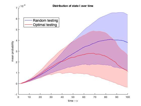
Figure 4: PCE and Optimal testing:(Left) Trade-off between the risk (objective function in (13)) versus
the testing budget (regularization parameter λ i.e., no. of tests). (Right) Distribution [mean with standard
deviation error band] of state I over time with random and optimal testing.
the PCE analysis.
In the right plot, we give the cardinality of the optimal testing prescription vector wT obtained, i.e, the
number of tests prescribed, as a function of the regularization parameter λ. The Matlab CVX package [24]
was used to solve the optimization problem in eqn (13) with functions as described before. We first observe
that, as we decrease λ, the cardinality of wT , i.e., the no. of prescribed tests increases. We can choose an
optimal λ value based on the available budget. Moreover, we observed that the method prescribes testing for
individuals with high uncertainty (individuals with high variance in the right plot of Fig. 2). These results
show that we can quantify the uncertainty in our model and prescribe appropriate testing.
In figure 4, the left plot in the figure presents the risk to budget trade-off by plotting the final value of
objective function in (13) we obtained for the optimal wt for different values of the regularization parameter
λ. We again chose n = 1000, T = 100, and other parameters as before. Decreasing λ increases the no.
of prescribed tests, and in turn the testing budget required. The plot shows that increasing the no. of tests
reduces the risk initially and after a point this reduction is minimal. The trade-off plot helps us to choose an
optimal λ (lowest testing budget) for an acceptable risk tolerance. The right plot in the Figure 4, presents
the distribution of the infection state I over time steps t when testing was conducted randomly (in blue) and
when optimal testing was prescribed at regular intervals (in red). We considered T = 100 time steps, and
in the first case, we performed random testing at each time instance. In the second case, we ran the PCE
analysis after every 10 time instances (use previous 10 random measurements to construct the PCE) and used
the optimal testing prescription in the next instance. We observe that in the second case, the mean infection
starts reducing sooner than the random testing. These results suggest that indeed prescribing optimal testing
can help control uncertainty and mitigate disease transmission.
Conclusions
In this study, we introduced a probabilistic SEIR model for disease transmission. The model represents
individual-level contact tracing information via dynamic graphs, where each individual represents a node
and interaction is described by edges. The S, E, I, R compartments are treated as probabilistic entities
as to capture uncertainty associated with the stochastic process of disease propagation, sparse testing, and
14model inadequacies. As illustrated by numerical simulations, this model can serve healthcare professionals
in issuance of early warnings to individuals who are likely exposed or infected by the virus. Furthermore,
the model identifies those individuals who are likely to be asymptomatic. We then proposed the use of
arbitrary Polynomial Chaos Expansion (aPCE) to quantify uncertainties in the model, while maintaining
computational scalability. By estimating the expected risk as well as minimizing uncertainty we prescribe
optimal testing for individuals under limited testing and tracing resources. The framework offers a decision
tool for balancing between immediate disease spread threat intervention and informed assessment of the
pandemic state. Lastly, the framework provides means for policy makers as to estimate the required testing
budget for a given acceptable risk tolerance and can be easily adapted to optimize vaccine distribution.
References
[1] D. Acemoglu, V. Chernozhukov, I. Werning, and M. D. Whinston. A multi-risk sir model with optimally targeted
lockdown. Technical report, National Bureau of Economic Research, 2020.
[2] R. Ahlfeld, B. Belkouchi, and F. Montomoli. Samba: sparse approximation of moment-based arbitrary polynomial
chaos. Journal of Computational Physics, 320:1–16, 2016.
[3] A. Alexanderian, N. Petra, G. Stadler, and O. Ghattas. A fast and scalable method for a-optimal design of
experiments for infinite-dimensional bayesian nonlinear inverse problems. SIAM Journal on Scientific Computing,
38(1):A243–A272, 2016.
[4] A. Alexanderian, N. Petra, G. Stadler, and O. Ghattas. Mean-variance risk-averse optimal control of systems
governed by pdes with random parameter fields using quadratic approximations. SIAM/ASA Journal on Uncertainty
Quantification, 5(1):1166–1192, 2017.
[5] H. Alsdurf, Y. Bengio, T. Deleu, P. Gupta, D. Ippolito, R. Janda, M. Jarvie, T. Kolody, S. Krastev, T. Maharaj,
et al. Covi white paper. arXiv preprint arXiv:2005.08502, 2020.
[6] Apple-Google. Apple-google exposure notification. https://www.google.com/covid19/
exposurenotifications/, https://www.apple.com/covid19/contacttracing/, 2020.
[7] J. M. Aronis, N. E. Millett, M. M. Wagner, F. Tsui, Y. Ye, J. P. Ferraro, P. J. Haug, P. H. Gesteland, and G. F.
Cooper. A bayesian system to detect and characterize overlapping outbreaks. Journal of biomedical informatics,
73:171–181, 2017.
[8] Y. Bengio, R. Janda, Y. W. Yu, D. Ippolito, M. Jarvie, D. Pilat, B. Struck, S. Krastev, and A. Sharma. The need for
privacy with public digital contact tracing during the covid-19 pandemic. The Lancet Digital Health, 2020.
[9] D. W. Berger, K. F. Herkenhoff, and S. Mongey. An seir infectious disease model with testing and conditional
quarantine. Technical report, National Bureau of Economic Research, 2020.
[10] I. Bistritz, D. Kahana, N. Bambos, I. Ben-Gal, and D. Yamin. Controlling contact network topology to prevent
measles outbreaks. In 2019 IEEE Global Communications Conference (GLOBECOM), pages 1–6. IEEE, 2019.
[11] K. Biswas and P. Sen. Space-time dependence of corona virus (covid-19) outbreak. arXiv preprint
arXiv:2003.03149, 2020.
[12] L. N. Carroll, A. P. Au, L. T. Detwiler, T.-c. Fu, I. S. Painter, and N. F. Abernethy. Visualization and analytics
tools for infectious disease epidemiology: a systematic review. Journal of biomedical informatics, 51:287–298,
2014.
[13] J. H. Cartwright and O. Piro. The dynamics of runge–kutta methods. International Journal of Bifurcation and
Chaos, 2(03):427–449, 1992.
[14] CDC. Cdc coronavirus disease 2019 (covid-19). https://www.cdc.gov/coronavirus/2019-ncov/
php/open-america/contact-tracing-resources.html, 2020.
15[15] Y.-C. Chen, P.-E. Lu, C.-S. Chang, and T.-H. Liu. A time-dependent sir model for covid-19 with undetectable
infected persons. arXiv preprint arXiv:2003.00122, 2020.
[16] L. Cirrincione, F. Plescia, C. Ledda, V. Rapisarda, D. Martorana, R. E. Moldovan, K. Theodoridou, and E. Canniz-
zaro. Covid-19 pandemic: Prevention and protection measures to be adopted at the workplace. Sustainability,
12(9):3603, 2020.
[17] G. Cohen and L. Horesh. Crowd sourced contact tracing, informing and prevention of virus contagion with privacy
preservation, 2020.
[18] G. F. Cooper, R. Villamarin, F.-C. R. Tsui, N. Millett, J. U. Espino, and M. M. Wagner. A method for detecting and
characterizing outbreaks of infectious disease from clinical reports. Journal of biomedical informatics, 53:15–26,
2015.
[19] T. Crestaux, O. Le Maıtre, and J.-M. Martinez. Polynomial chaos expansion for sensitivity analysis. Reliability
Engineering & System Safety, 94(7):1161–1172, 2009.
[20] B. J. Debusschere, H. N. Najm, P. P. Pẽbay, O. M. Knio, R. G. Ghanem, and O. P. Le Maıtre. Numerical challenges
in the use of polynomial chaos representations for stochastic processes. SIAM journal on scientific computing,
26(2):698–719, 2004.
[21] DP3T. Dp3t - decentralized privacy-preserving proximity tracing. https://github.com/DP-3T/
documents, 2020.
[22] D. Faranda and T. Alberti. Modelling the second wave of covid-19 infections in france and italy via a stochastic
seir model. arXiv preprint arXiv:2006.05081, 2020.
[23] R. G. Ghanem and P. D. Spanos. Stochastic finite elements: a spectral approach. Courier Corporation, 2003.
[24] M. Grant and S. Boyd. Cvx: Matlab software for disciplined convex programming, 2009.
[25] G. Großmann, M. Backenköhler, and V. Wolf. Importance of interaction structure and stochasticity for epidemic
spreading: A covid-19 case study. In International Conference on Quantitative Evaluation of Systems, pages
211–229. Springer, 2020.
[26] V. Guerrieri, G. Lorenzoni, L. Straub, and I. Werning. Macroeconomic implications of covid-19: Can negative
supply shocks cause demand shortages? Technical report, National Bureau of Economic Research, 2020.
[27] R. Gupta and S. K. Pal. Trend analysis and forecasting of covid-19 outbreak in india. medRxiv, 2020.
[28] C. J. Jones, T. Philippon, and V. Venkateswaran. Optimal mitigation policies in a pandemic: Social distancing and
working from home. Technical report, National Bureau of Economic Research, 2020.
[29] A. Kaintura, T. Dhaene, and D. Spina. Review of polynomial chaos-based methods for uncertainty quantification
in modern integrated circuits. Electronics, 7(3):30, 2018.
[30] A. Katok and B. Hasselblatt. Introduction to the modern theory of dynamical systems. Number 54. Cambridge
university press, 1997.
[31] W. Kermack and A. McKendrick. Contributions to the mathematical theory of epidemics – i. Bulletin of
Mathematical Biology, 53(1-2):33–55, 1991.
[32] W. Kermack and A. McKendrick. Contributions to the mathematical theory of epidemics – ii. the problem of
endemicity. Bulletin of Mathematical Biology, 53(1-2):57–87, 1991.
[33] W. Kermack and A. McKendrick. Contributions to the mathematical theory of epidemics – iii. further studies of
the problem of endemicity. Bulletin of Mathematical Biology, 53(1-2):89–118, 1991.
[34] J. Kwon, C. Grady, J. T. Feliciano, and S. J. Fodeh. Defining facets of social distancing during the covid-19
pandemic: Twitter analysis. Journal of Biomedical Informatics, page 103601, 2020.
16[35] S. Lalmuanawma, J. Hussain, and L. Chhakchhuak. Applications of machine learning and artificial intelligence
for covid-19 (sars-cov-2) pandemic: A review. Chaos, Solitons & Fractals, page 110059, 2020.
[36] R. Li, S. Pei, B. Chen, Y. Song, T. Zhang, W. Yang, and J. Shaman. Substantial undocumented infection facilitates
the rapid dissemination of novel coronavirus (sars-cov-2). Science, 368(6490):489–493, 2020.
[37] J. Liu, L. Wang, Q. Zhang, and S. T. Yau. The dynamical model for covid-19 with asymptotic analysis and
numerical implementations. Applied Mathematical Modelling, 2020.
[38] L. López and X. Rodó. The end of social confinement and covid-19 re-emergence risk. Nature Human Behaviour,
4(7):746–755, 2020.
[39] L. López and X. Rodo. A modified seir model to predict the covid-19 outbreak in spain and italy: simulating
control scenarios and multi-scale epidemics. Available at SSRN 3576802, 2020.
[40] X. Mei, H.-C. Lee, K.-y. Diao, M. Huang, B. Lin, C. Liu, Z. Xie, Y. Ma, P. M. Robson, M. Chung, et al. Artificial
intelligence–enabled rapid diagnosis of patients with covid-19. Nature Medicine, pages 1–5, 2020.
[41] NHS. NHS covid-19 app. https://www.nhsx.nhs.uk/covid-19-response/
nhs-covid-19-app/, 2020.
[42] S. Oladyshkin, H. Class, and W. Nowak. Bayesian updating via bootstrap filtering combined with data-driven
polynomial chaos expansions: Methodology and application to history matching for carbon dioxide storage in
geological formations. Computational Geosciences, 08 2013.
[43] S. Oladyshkin and W. Nowak. Data-driven uncertainty quantification using the arbitrary polynomial chaos
expansion. Reliability Engineering & System Safety, 106:179–190, 2012.
[44] S. Oladyshkin, P. Schröder, H. Class, and W. Nowak. Chaos expansion based bootstrap filter to calibrate co2
injection models. Energy Procedia, 40:398–407, 2013.
[45] L. Peng, W. Yang, D. Zhang, C. Zhuge, and L. Hong. Epidemic analysis of covid-19 in china by dynamical
modeling. arXiv preprint arXiv:2002.06563, 2020.
[46] PEPP. Pan-european privacy-preserving proximity tracing. https://pepp-pt.org/, 2020.
[47] D. Pradhan, P. Biswasroy, G. Ghosh, G. Rath, et al. A review of current interventions for covid-19 prevention.
Archives of medical research, 2020.
[48] V. M. Preciado, M. Zargham, C. Enyioha, A. Jadbabaie, and G. Pappas. Optimal vaccine allocation to control
epidemic outbreaks in arbitrary networks. In 52nd IEEE conference on decision and control, pages 7486–7491.
IEEE, 2013.
[49] T. Sardar, S. S. Nadim, and J. Chattopadhyay. Assessment of 21 days lockdown effect in some states and overall
india: a predictive mathematical study on covid-19 outbreak. arXiv preprint arXiv:2004.03487, 2020.
[50] I. B. Schwartz, J. H. Kaufman, K. Hu, and S. Bianco. Predicting the impact of asymptomatic transmission,
non-pharmaceutical intervention and testing on the spread of covid19. medRxiv, 2020.
[51] G. Shulkind, L. Horesh, and H. Avron. Experimental design for nonparametric correction of misspecified
dynamical models. SIAM/ASA Journal on Uncertainty Quantification, 6(2):880–906, 2018.
[52] P. X. Song, L. Wang, Y. Zhou, J. He, B. Zhu, F. Wang, L. Tang, and M. Eisenberg. An epidemiological forecast
model and software assessing interventions on covid-19 epidemic in china. MedRxiv, 2020.
[53] J. T. Thorson, K. Ono, and S. B. Munch. A bayesian approach to identifying and compensating for model
misspecification in population models. Ecology, 95(2):329–341, 2014.
[54] C. Tian, Q. Zhang, and L. Zhang. Global stability in a networked sir epidemic model. Applied Mathematics
Letters, page 106444, 2020.
17You can also read