Dynamic Thermal Line Rating: Using the Weather to Increase Transmission Line Capacity - FACULTY OF ENGINEERING Leanne Dawson January 20, 2020

FACULTY OF ENGINEERING

Dynamic Thermal Line Rating:
Using the Weather to Increase
Transmission Line Capacity
Leanne Dawson
January 20, 2020

Outline

 What is DTLR?
 Rating Methods
 DTLR Implementation and Challenges
 U of C DTLR Research Project

 2

Background

 Utilities are
 investigating
 As more renewable Dynamic Thermal
 methods to increase
 generation is added Line Rating (DTLR) is
 transmission line
to the grid in Alberta one solution
 capacity while
 minimizing cost

 3

Types of Line Ratings

 The type of line rating that is used is dependent on
 the length of the transmission line
 — Thermal limit (short lines – under 80 km)
 — Voltage limit (medium lines – between 80 and 250 km)
 — Stability limit (long lines – over 250 km)
 Dynamic thermal line rating is based on the thermal
 limit of a line, so is typically only used for short lines

 4

What is Dynamic Thermal Line Rating (DTLR)?

 http://www.studyelectrical.com/2016/01/sag-in-overhead-transmission-conductor-lines.html
 https://clipartpig.com/download/ThcokA3
 https://pixabay.com/en/wind-energy-renewable-energy-wind-2029621/

What is DTLR?

Presently, utilities use:
 Reasonable
 outer-range IEEE/CIGRE
 Static Rating
environmental Model
 conditions

Switching to a DTLR requires:

 Dynamic
 Weather IEEE/CIGRE
 Thermal Line
 station data Model
 Rating

 6

DTLR Benefits

 Increased system visibility
 Reduced aging
 Network planning
 Network reliability
 Increased wind penetration
 Icing and galloping detection
 Maintaining clearance

 7

DTLR Methods

 DTLR can be calculated using either indirect or direct
 measurements
 Direct measurements include:
 — Conductor temperature
 — Sag
 Indirect measurements include:
 — Line tension
 — Weather conditions
 — Fundamental frequency
 — Electromagnetic waves
 — Synchrophasor data

 8

Sag Methods

 These methods either directly or indirectly measure
 the position of the line to compare to minimum
 clearance requirements
 There are commercial products available that can
 measure/calculate the sag of a line using:
 — Line tension (CAT-1)
 — LiDAR (Lindsey Manufacturing)
 — Fundamental frequency (Ampacimon)
 — Electromagnectic waves (LineVision)

 9

Weather-based Method

 Uses multiple weather parameters as input to a
 thermodynamic model (IEEE Standard 738-2012) to
 calculate the conductor temperature
 Weather variables include:
 — Wind speed
 — Wind direction
 — Ambient temperature
 — Solar radiation
 Historical weather data can be used to interpolate or
 predict the rating

 10

IEEE Model

 IEEE Standard 738:
 2
 I R(Tc )+ q s = q c + q r
 Where:
 — c is the heat removed by convection (air movement)
 — r is the heat removed by radiation to surrounding air
 — s is the heat gained from solar radiation from the sun
 — 2R( c) is the heat generated by the electron current flow
 in the conductor
 — Tc is the core temperature of the conductor

 11

Convection Cooling

  Natural convection (no wind):
=qcn 3.645 p f D 0.5 0.75
 (Tc − Ta ) 1.25

  Low wind:
   DVw p f  
 0.52

 1.01 + 0.0372 
 qc1 =   k f K angle (Tc − Ta )
   µ  
   f  
  High wind:
   DVw p f 
 0.6
 
 qc 2 0.0119    k f K angle (Tc − Ta )
   µ 
   f  
 12

Convection Cooling

 The parameters pf (air density), f (dynamic
 viscosity), f (thermal conductivity) are dependent
 on ambient temperature and conductor type
 Kangle is a function of the wind direction
 The convection cooling term is a non-linear function
 of the wind speed

 13

Radiant Cooling

  Tc + 273 4  Ta + 273 4 
 qr 0.0178 Dε   −  
  100   100  

 Radiant cooling is dependent on conductor
 properties, diameter (D) and emissivity (ε), and
 temperature, conductor (Tc) and ambient (Ta)

 14

Solar Heat Gain

 qs = α Qse sin (θ ) A '

 The solar heat gain can be calculated using the above
 equation
 The solar heat gain is dependent on absorptivity (α),
 solar radiation (Qse), elevation and time of day
 Solar radiation can be measured by the weather
 station

 15

Current Heating

 Current heating is dependent on current and
 resistance
 Resistance is a function of conductor temperature

 R(Tc ) = Rref (1 + α (Tc − Tref ))
 Previous research has investigated implementing
 temperature-dependent resistance in optimal power
 flow

 16

Transient Equation

 The previous equation is based on steady state
 The transient response for the conductor
 temperature due to a step change in current is:

 I R(Tc ) − qc (Tc ) − qr (Tc ) + qs
 2
 ∆Tc * ∆t
 mC p
 The transient response is a function of the heat
 capacity of the line
 The time constant is 5-15 minutes, depending on the
 weather conditions used
 17

Ambient-Adjusted Ratings

 Another form of DTLR is to only use changes in
 ambient temperature
 Can alleviate some of the risk associated with DTLR,
 as the variations in wind speed/direction are ignored
 Does not have as high of an increase compared to
 using a full DTLR

 18

Other Methods

 Synchrophasor data can also be used to calculate a
 DTLR
 Phasor Measurement Unit (PMU) data provides the
 voltage and current at different points in the grid
 The difference in voltage at two points can be
 combined with the relationship between resistance
 and temperature to determine the conductor
 temperature indirectly

 19

DTLR Implementation

 To implement DTLR on a transmission line, there are
 three main methods:
 — Find the hottest-spot on the transmission line (limiting
 span) to determine where to install a device to determine
 what the minimum rating would be for the entire line
 — Interpolate the rating over the terrain using multiple
 weather stations and mathematical modeling
  Idaho National Lab (INL) uses computational fluid dynamics
 (CFD) to interpolate wind data
 — Install sufficient number of devices to cover desired line

 20

DLTR Prediction

 Difficult to implement DTLR in real-time
 Some commercial DTLR products have prediction
 capabilities built-in
 Most prediction methods are based on historical
 weather data
 Time horizon can be 1 hour ahead up to 48 hours
 ahead
 — The longer the time horizon, the lower the ampacity will
 be to preserve accuracy

 21

DTLR Challenges

 The limiting span can be difficult to determine
 — Depends on the terrain and predominant wind direction
 — Interpolating weather data can be computationally
 intensive
 — Installing multiple devices can be expensive, depending on
 the technology used
 Collecting sufficient weather data
 Communication between devices and EMS
 Integrating a dynamic rating into EMS

 22

Research Project

 The DTLR Research Project is focused on investigating
 the implementation of DTLR in Alberta
 Components of the project:
 — Fuzzy DTLR Prediction
 — Transient Impact
 — Spatial DTLR Patterns

 23

Gathering Weather Data

Environment
 Canada
Weather data

 http://weclipart.com/power+lines+clipart
 http://clipground.com/weather-station-clipart.html
 https://fabulousbydesign.net/printable-map-of-alberta/

Transient Model Validation

 Transient model validated using conductor
 temperature data from ATCO
 The data was collected using a GE line monitoring
 relay mounted on a transmission line
 This relay measures the line current, the conductor
 temperature and the weather conditions

 25

Conductor Temperature Validation

 26

Using DTLR Transient Method

 Investigating the transient thermal impact on
 transmission lines when environmental conditions
 drastically change
 Investigating the thermal risk of updating the rating
 every hour using different confidence levels
 Used 3-minute weather data provided by AltaLink to
 compare the hourly predicted rating over one winter
 day to real-time transient conditions

 27

Weather Data
 50

 40

 Wind Speed (m/s)
 30

 20

 10

 0
 0 2 4 6 8 10 12 14 16 18 20 22 24

 80
Wind Direction (deg)

 60

 40

 20

 0
 0 2 4 6 8 10 12 14 16 18 20 22 24

 6
 Ambient Temperature (degC)

 4

 2

 0

 -2

 0 2 4 6 8 10 12 14 16 18 20 22 24

 Time (h)

 28

Fuzzy Prediction Model

 A fuzzy clustering model is used for hour-ahead DTLR
 prediction
 Historical weather data (wind speed, wind direction
 and ambient temperature) are fed into the model
 A fuzzy model is used to quantify the hourly
 variations in weather variables
 Different confidence levels are defined based on the
 desired level of risk

 29

Predicted Ampacity
 300

Maximum Predicted Ampacity (% of static limit) 250

 200

 150

 100
 95% Confidence
 85% Confidence
 75% Confidence
 50
 65% Confidence
 55% Confidence

 0
 0 2 4 6 8 10 12 14 16 18 20 22 24

 Time (h)
 30

Comparing Transient and Steady-State
 110

 Quasi-Steady-State Thermal Model
 100
 Transient Thermal Model

 90

 80

 70
Conductor Temperature (degC)

 60

 50

 40

 30

 20

 10

 0
 0 2 4 6 8 10 12 14 16 18 20 22 24

 Time (h)

 Comparing transient and steady-state conductor
 temperature calculations using 95% confidence level 31

Transient Tc for Two Confidence Levels

 1800 Real-time 160

 95% Confidence 85% Confidence
 85% Confidence 95% Confidence
 1600 140

 120
 1400

 Conductor Temperature (degC)
 100
 1200
Ampacity (A)

 80
 1000

 60

 800

 40

 600
 20

 400
 0
 0 2 4 6 8 10 12 14 16 18 20 22 24 0 2 4 6 8 10 12 14 16 18 20 22 24
 Time (h) Time (h)

 Comparing real-time ampacity to two Transient conductor temperature for
 different confidence levels 85 and 95% confidence levels

 32

Summary of Results

 Transient method is more accurate than using the
 steady-state method when compared to real-time
 conductor temperature measurements
 Changes in conductor temperature are mainly
 dependent on changes in wind speed and wind
 direction
 Trade-off between excepted risk and ampacity
 increase

 33

DTLR Patterns

 Is DTLR available when we need it, where we need
 it?
 Future congestion due to wind isn’t necessarily next
 to the wind farm
 If we add wind farms to Area A, do the weather
 conditions that produce the power correlate to
 favorable weather conditions in Area B, where the
 congestion is?
 How does the potential DTLR increase change over
 an area?

 34

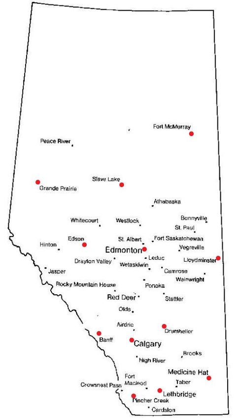
Applicability of DTLR in Alberta

 Purpose is to investigate the applicability of DTLR in
 different areas of the province
 Spatial Impact
 — 4 different test cases (3 locations each)
 Temporal Impact
 — 4 different locations over 4 different years
 Directional impact
 — 2 different locations, 2 different directions each

 35

Weather Station Locations

Environment
 Canada
Weather data

 https://fabulousbydesign.net/printable-map-of-alberta/

Spatial Impact
 1400 Pincher Creek Lethbridge Medicine Hat 1400
Ampacity (A)

 Ampacity (A)
 1200 1200

 1000 1000

 5 10 15 20 5 10 15 20

 1100 Banff Calgary Drumheller 1100

 1000 1000
Ampacity (A)

 Ampacity (A)
 900 900

 800 800

 700 700
 5 10 15 20 5 10 15 20

 1300 Edson Edmonton Lloydminster
 1300

 1200 1200
Ampacity (A)

 Ampacity (A)
 1100 1100

 1000 1000

 900 900

 5 10 15 20 5 10 15 20

 1300 1300
 Grande Prairie Slave Lake Fort MacMurray
 1200 1200
Ampacity (A)

 Ampacity (A)
 1100 1100

 1000 1000

 900 900
 5 10 15 20 5 10 15 20

 Time (hours) Time (hours)

 a) b)

 Average Hourly DTLR in Different Locations for a) Summer b) Winter
 37

Temporal Impact
 2200 2200

 2000
 Summer 2000
 Winter 2017
 2007
 1997
 1987
 1800 1800

 1600 1600

 1400 1400

 Calgary
 Ampacity (A)

 Ampacity (A)
 1200 1200

 1000 1000

 800 800

 600 600

 400 400
 0 0.2 0.4 0.6 0.8 1 0 0.2 0.4 0.6 0.8 1

 % of Time Rating is Below % of Time Rating is Below
 2000 2200

 2017
 2007
 2000
 1800
 1997
 1987
 1800
 1600

 1600
 1400

Edmonton 1400
 Ampacity (A)

 1200
 Ampacity (A)
 1200

 1000
 1000

 800
 800

 600
 600

 400 400
 0 0.2 0.4 0.6

 % of Time Rating is Below
 0.8 1 0 0.2 0.4 0.6

 % of Time Rating is Below
 0.8 1
 38

Impact of Line Direction - Calgary
1987 NORTH
 NORTH 2017
 15%
 15%

 10%
 10%

 5%
 5%

 20 - 22
 WEST EAST 18 - 20
 WEST EAST 18 - 20
 16 - 18
 16 - 18
 14 - 16
 14 - 16
 12 - 14
 12 - 14
 10 - 12
 10 - 12
 8 - 10
 8 - 10
 6-8
 6-8
 4-6
 4-6
 2-4
 2-4
 0-2 SOUTH 0-2
 SOUTH

 a) b)

 2200
 Summer 2200
 Winter N-S 2017
 2000 2000 E-W 2017
 N-S 1987
 1800 E-W 1987
 1800

 1600
 1600

 1400
 1400
 Ampacity (A)

 Ampacity (A)

 1200

 1200
 1000

 1000
 800

 800
 600

 400 600

 200 400
 0 0.2 0.4 0.6 0.8 1 0 0.2 0.4 0.6 0.8 1 39
 % of Time Rating is Below % of Time Rating is Below

Impact of Line Direction - Edmonton
1987 2017
 NORTH NORTH

 15% 6%

 10% 4%

 5% 2%

 20 - 22

 WEST EAST 18 - 20
 WEST EAST
 16 - 18 16 - 18

 14 - 16 14 - 16

 12 - 14 12 - 14

 10 - 12 10 - 12
 8 - 10
 8 - 10
 6-8
 6-8
 4-6
 4-6
 2-4
 2-4
 SOUTH 0-2
 SOUTH 0-2

 a) b)

 2000
 Summer 2200
 Winter N-S 2017

 2000 E-W 2017
 1800
 N-S 1987
 E-W 1987
 1800
 1600

 1600
 1400

 1400
 Ampacity (A)

 Ampacity (A)

 1200

 1200

 1000
 1000

 800
 800

 600
 600

 400 400

 40
 0 0.2 0.4 0.6 0.8 1 0 0.2 0.4 0.6 0.8 1

 % of Time Rating is Below % of Time Rating is Below

Summary of Results

 The potential increase provided by using a DTLR is
 dependent on the location and the prevailing
 weather conditions for each year
 The static limit is not sufficient, as for every test case
 the static limit was exceeded by 7-20% when using
 two seasonal limits
 The diurnal patterns for the average hourly DTLR vary
 based on location
 Changing the line orientation from north-south to
 east-west makes minimal difference on the overall
 yearly potential DTLR values

 41

DTLR Clustering Analysis

 Received wind speed and direction data from Pan-
 Canadian Wind Integration study
 Included 9,570 files of data for Alberta
 Data is sampled every 10 minutes over 2008-10
 Number of data points is reduced based on density
 of data points
 Fed data into DTLR model
 Clustered DTLR results using k-means clustering

 42

Clustering Method

 K-means clustering is an unsupervised learning
 method, whose aim is to separate the input data into
 a specified number of groups with equal variance
 Unsupervised clustering methods are used when the
 cluster identity of each point is not pre-defined
 K-means clustering is selected for this analysis
 because of its ability to handle a large number of
 samples
 One of the challenges with using unsupervised
 learning models is the need to specify the number of
 clusters

 43

Cluster Number Comparison

 44

Monthly Cluster Results

 45

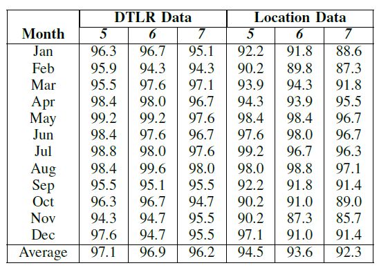
Predicting DTLR

Accuracy of DTLR Classification Using Location Data Compared to Historical
 DTLR For Different Numbers of Clusters

 46

Summary of Results

 Data patterns change based on number of clusters
 — Six clusters are selected for this analysis
 DTLR patterns change for each month
 More distinct clusters based on location during the
 summer months compared to the winter months
 Prediction accuracy is higher using DTLR data
 compared to location, but the difference is smaller
 for the summer months

 47

Summary

 DTLR is one solution to maximize transmission line
 capacity while minimizing cost
 Challenges exist in widespread implementation
 Research is being done to investigate using machine
 learning for temporal and spatial prediction
 More work needs to be done to translate this work
 into industry practice

 48

Acknowledgment

 I would like to thank NSERC and our industry
 partners for their support of this project
 I would also like to acknowledge the other
 contributors to this portion of the project, Soheila
 Karimi and Dr. Andy Knight, both from the U of C

 49

50