Effects of confinement on the dynamics and correlation scales in kinesin-microtubule active fluids
←
→
Page content transcription
If your browser does not render page correctly, please read the page content below
PHYSICAL REVIEW E 104, 034601 (2021)

 Effects of confinement on the dynamics and correlation scales in kinesin-microtubule active fluids

                         Yi Fan ,1 Kun-Ta Wu,2 S. Ali Aghvami ,3 Seth Fraden ,3 and Kenneth S. Breuer1,*
               1
                   Center for Fluid Mechanics, School of Engineering, Brown University, Providence, Rhode Island 02912, USA
                         2
                           Department of Physics, Worcester Polytechnic Institute, Worcester, Massachusetts 01609, USA
                                  3
                                    School of Physics, Brandeis University, Waltham, Massachusetts 02453, USA

                                  (Received 15 March 2021; accepted 9 August 2021; published 2 September 2021)

                  We study the influence of solid boundaries on dynamics and structure of kinesin-driven microtubule active
               fluids as the height of the container, H , increases from hundreds of micrometers to several millimeters. By
               three-dimensional tracking of passive tracers dispersed in the active fluid, we observe that the activity level,
               characterized by velocity fluctuations, increases as system size increases and retains a small-scale isotropy.
               Concomitantly, as the confinement level decreases, the velocity-velocity temporal correlation develops a strong
               positive correlation at longer times, suggesting the establishment of a “memory”. We estimate the characteristic
               size of the flow structures from the spatial correlation function and find that, as the confinement becomes
               weaker, the correlation length, lc , saturates at approximately 400 microns. This saturation suggests an intrinsic
               length scale which, along with the small-scale isotropy, demonstrates the multiscale nature of this kinesin-driven
               bundled microtubule active system.

               DOI: 10.1103/PhysRevE.104.034601

                         I. INTRODUCTION                                      The second broad category of geometries are three-
                                                                          dimensional annular “race-tracks”, which have a planform, or
    Active fluids, and more specifically, cytoskeletal net-
                                                                          x-y geometry, in the form of a circle, square, ratchet, toroid,
works of actin filaments or microtubules, exhibit large-
                                                                          or long channel but are confined in the transverse, or y-z
scale nonequilibrium dynamics driven by mesoscopic active
                                                                          plane, by solid boundaries. Such confinement can transform
stresses, which are generated by nanoscale motion of molec-
                                                                          the chaotic dynamics of three-dimensional (3D) bulk isotropic
ular motors [1–6]. Boundaries can dramatically transform
                                                                          fluids into long-ranged and long-lived coherent flows and
the dynamics of such cytoskeletal active networks generating
                                                                          be capable of transporting materials over macroscopic scales
coherent flow patterns or self-organized states including, for
                                                                          [22,23]. The emergence of such coherent flows appears to be
example vortical, spiral, swirling, and other patterns [7–13].
                                                                          determined by a scale-invariant criterion that depends on the
From a biological perspective, the formation of these patterns
                                                                          aspect ratio of the confining geometry.
underlie biological phenomena such as spindle formation or
                                                                              To understand these effects, it is essential to elucidate
cytoplasmic streaming [14–18], while from a more physical
                                                                          the influence of the hard wall boundaries on the active fluid
perspective, active fluids provide a novel system that converts
                                                                          structure and dynamics and to quantify the changing length
chemical energy into mechanical work at the molecular scale
                                                                          and time scales that emerge in response to confinement. In
and then generates mesoscopic activity at much larger scales,
                                                                          this work we report on the behavior of a 3D bulk active
mediated by the short- and long-range interactions intrinsic to
                                                                          fluid system as it is subjected to decreasing confinement in
the specific active medium.
                                                                          one direction. To study this, we have conducted a series of
    A particularly versatile model system of active fluids is
                                                                          experiments in cuboid channels whose horizontal dimension
composed of ∼100 μm long bundles of short microtubule
                                                                          is large (2 or 4 mm) compared to any internal scale of the
filament, each approximately 1.5 μm long. These bundles
                                                                          active medium, but whose vertical dimension, H, ranges from
extend, buckle, and fray, driven by the motion of kinesin
                                                                          a highly confined geometry (H = 100 μm) to one whose
molecular motors [19]. Most of the studies of the isotropic
                                                                          scale is large and comparable to the horizontal system scale
active phase using this long-lasting active fluid have focused
                                                                          (H > 2 mm). In each of these test geometries (except the
on two different configurations: two-dimensional unconfined
                                                                          largest geometry case) we tracked passive tracer particles in
thin-film and three-dimensional annular geometries. The thin-
                                                                          all three dimensions and calculated their transport, spatial and
film systems are unconfined in the horizontal plane (x-y) and
                                                                          temporal correlation in the active fluids.
measure 100 μm or less in the vertical (z) axis. The vertical
confinement is achieved either using an oil film or a solid
boundary. This geometry has been used to characterize the                                 II. MATERIALS AND METHODS
dynamics and structure of the system for a variety of different
                                                                                                    A. Active fluids
microscopic constituents [20,21].
                                                                             Active fluids composed of microtubule filaments, kinesin-
                                                                          streptavidin motor clusters, depletion agents (Pluronic F-127,
                                                                          Sigma, P2443), and an adenosine triphosphate (ATP) re-
 *
     kenneth_breuer@brown.edu                                             generation system. Pluronic micelles force the microtubule

2470-0045/2021/104(3)/034601(8)                                    034601-1                                 ©2021 American Physical Society
FAN, WU, AGHVAMI, FRADEN, AND BREUER PHYSICAL REVIEW E 104, 034601 (2021)
TABLE I. Summary of experimental details for each channel. Channels i–vii have increasing chamber height, H , with the measurement
position, z/H , at (approximately) the channel center. Channels vi-a and vi-b have the same dimensions as channel vi, but the observation
position is closer to one of the boundaries.
Chamber dimension Objective Observation position Tracer
Index W L H WD z diameter Tracking
number (mm) (mm) (mm) (mm) NA (mm) z/H (μm) dimensions
i 2.0 2.0 0.1 1.0 0.75 0.05 0.5 1.0 3D
ii 2.0 2.0 0.3 1.0 0.75 0.15 0.5 1.0 3D
iii 2.0 2.0 0.5 1.0 0.75 0.25 0.5 1.0 3D
iv 2.0 2.0 1.0 1.0 0.75 0.50 0.5 1.0 3D
v 2.0 2.0 1.5 1.0 0.75 0.75 0.5 1.0 3D
vi 2.0 2.0 2.0 1.0 0.75 0.80a 0.4 1.0 3D
vi-a 2.0 2.0 2.0 1.0 0.75 0.05 0.025 1.0 3D
vi-b 2.0 2.0 2.0 1.0 0.75 0.15 0.075 1.0 3D
vii 4.0 4.0 4.0 6.9 0.45b 2.00 0.5 2.9 2D
a
Objective Nikon CFI Plan Apo VC 20×. Its working distance (WD) restricted the observation position z.
b
Objective Nikon CFI S Plan Fluor ELWD 20×. Its numerical aperture (NA) restricted the tracking dimension to two-dimensional.
filaments to form bundles [24]. Kinesin-streptavidin motor the fluorescent tracers. Light from a high power LED source
clusters simultaneously bind to and walk along neighbor mi- (405 nm, Thorlabs, DC4100) was directed through a narrow-
crotubule filaments, inducing a sliding motor force between band filter to an air immersion objective (either Nikon CFI S
antipolar filaments. The active stress generated by thousands Plan Fluor ELWD 20×, NA = 0.45, WD = 6.9 mm or Nikon
of molecular motors drives the system out of equilibrium. The CFI Plan Apo VC 20×, NA = 0.75, WD = 1.0 mm). The
ATP regeneration system maintains the ATP concentration in emission from the fluorescent tracers was directed through a
the active fluid which ensures that the kinesin motors step narrow-band emission filter and recorded using an sCMOS
at constant speed for the duration of the experiment. All of camera (PCO-Tech, PCO edge 5.5, 2560 × 2160 pixels) at
the experiments presented here used an active fluid with a 10 Hz.
constant concentration of microtubules (1.3 mg/ml), kinesin Tracer particles in the focal plane appear as sharp spots
(1.5 μM), and ATP (1.4 mM). Complete details on the active in the camera image while particles located away from the
material preparation are described in Appendix A. We dis- focal plane appear as “Airy rings” [25] whose diameter can
persed ∼0.001% (v/v) spherical colloidal fluorescent tracers be accurately correlated with the particle position above or
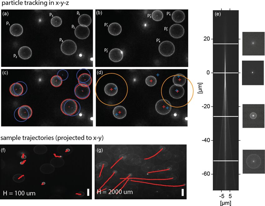
(2.9 μm diameter, 395 nm/428 nm, Bangs Laboratories, or below the focal plane [26,27] [Figs. 1(a) and 1(b)]. A typical
1 μm diameter, 412 nm/447 nm, Thermal Fisher Scientific) in image contained 30 particles, each of which was tracked in
the active fluid, with the tracer size determined by the channel three dimensions using its position in the image and the size
size and target observation region. of the tracer’s point spread function. The ring size was deter-
mined using a Sobel edge detection algorithm and the Circle
B. Test enclosure Hough Transform [28,29] [Figs. 1(c) and 1(d)]. A reference
library, which relates the Airy ring size to the tracer’s distance
Test chambers, consisting of a rectangular cavity mea- from the focal plane, was built [Fig. 1(e)] by z-scanning a
suring 2 by 2 mm (x-y), with a height (z) that varied from 1-μm tracer particle immobilized in agarose gel with 0.1-μm
H = 100 μm to 2 mm [Table I (i–vi)] and a cube measuring intervals using the piezo z-drive. The agarose gel is 1% (w/w)
4 mm in each of the three dimensions [Table I (vii)] were with the same refractive index as the active fluid medium.
fabricated from cyclic olefin copolymer (COC) sheets using Although it has a weblike structure, the underlying micro-
a CNC mill (MDA Precision LLC, Model V8-TC8 3-axis). tubule network is dilute and spatially homogeneous and can
The active fluids were loaded into the chamber which was be safely considered to be optically uniform. The Airy rings
then sealed using a glass slide (Fisher scientific, 12-542C). To recorded are uniform in intensity and are circular (See Sup-
ensure a consistent surface condition, all channels and cover plemental Material videos 1 and 2 [30]), confirming that there
slides were coated with polyacrylamide before experiments is no optical distortion that would be introduced by spatial
[19,20] (see Appendix B). The assembly was held onto the variations in the optical properties of the active fluid. The
microscope stage by a machined aluminum plate with a poly- resultant measurement and tracking system could determine
dimethylsiloxane layer (∼1-mm thickness placed between the the tracer location within a 350 μm × 350 μm × ∼ 40μm
glass and aluminum to provide stress relief). observation volume, with an accuracy of 0.2 μm in the x-y
plane and 0.4 μm in the z direction. For the largest geometry
C. Measurement procedures [channel vii, Table I], the large value of H required the use
An epifluorescence microscope (Nikon TE 200 eclipse) of a microscope objective with a long working distance. For
equipped with a z-scanning system (Piezo z-drive, Physik this case, the numerical aperture did not allow for detection
Instrumente, Model P-725) was used to observe the motion of of the Airy rings and restricted the particle tracking to two
034601-2EFFECTS OF CONFINEMENT ON THE DYNAMICS … PHYSICAL REVIEW E 104, 034601 (2021)
FIG. 1. Example of particle tracking in three dimensions. [(a) and (b)] Raw images taken at two successive times illustrating the sparse
seeding of tracer particles. Particle positions are indicated by the Airy rings. (c) The center and size of each ring is detected using Sobel
edge detection and the Hough circle transform. (d) Particles are tracked according to a nearest-neighbor algorithm. (e) The z location of each
particle is localized using the library of ring sizes vs. distance from the focal plane obtained from a calibration. [(f) and (g)] Two samples of
particle tracks, taken from a shallow and a deep test geometry (H = 100, 2000 μm) illustrating the qualitative change in particle mobility due
to confinement. The scale bar represents 40 μm.
dimensional. In addition, the field of view was enlarged to and H = 0.1 mm. The out-of-focus tracers were tracked from
700 μm × 700 μm in the horizontal plane. frame to frame in three dimensions based on their Airy ring
Tracer particle trajectories were assembled from a se- sizes. As expected, the MSD increased linearly with time
quence of images using the “nearest-neighbor” method [31]
and velocities in all three directions (ui = ux , uy , uz ) were
calculated using finite differences. Following the turbulence 10
literature [32], velocities were decomposed into mean com- 1 μm, 2x2x2 mm 3
1 μm, 2x2x0.1 mm3
ponent and fluctuating component which is a function of 5 2.9 μm, 4x4x4 mm3
experiment time t: ui (t ) = ui + ui (t ), where ui denotes an
MSD [μm 2 ]
average over all particles tracked during a period of constant
system activity [t = 2000–5600 s, Fig. 3(a)]. The variance 1
of the velocity, ui2 ≡ σi2 = [ui (t ) − ui ]2 , was computed by 1
averaging over all particles tracked during the same time
period.
0.5 1 2 5
Time lag [s]
III. RESULTS AND DISCUSSION
FIG. 2. Normalized mean-square displacements (MSDs) of 1-
A. Validation of measurement system
and 2.9-μm particles diffusing in water and tracked using the
To validate the three-dimensional measurement system, we Airy-disk three-dimensional tracking technique. The MSDs are nor-
recorded the Brownian motion of fluorescent tracers (1-μm malized by the size of particle (1-μm or 2.9-μm diameter), and the
diameter or 2.9-μm diameter) diffusing in deionized (DI) wa- error bars indicate standard errors of the averaging over all tracked
ter in three different COC chambers: H = 4 mm, H = 2 mm, particles.
034601-3FAN, WU, AGHVAMI, FRADEN, AND BREUER PHYSICAL REVIEW E 104, 034601 (2021)
(a) i iv vi vii (b) (a) (b)
vi-a u
¯x ū y ū z σx σy σz
vi-b 1 8
120 120
T = [t s , t e]
fluctuation, σ [μm/s]
i ii iii iv v vi vii 7
100 100
mean, u [μm/s]
vi-a 0.5 6
e || [(μm/s) 2 ]
vi-b
e || [(μm/s) 2 ]
80 80
5
0
60 60 4
40 40 -0.5 3
20 20 2
-1 10
0 0 0 1 2 3 4 1 2 3 4
0 4000 8000 12000 0 1 2 3 4 channel height, H [mm] channel height, H [mm]
experiment time [s] channel height, H [mm]
FIG. 4. (a) Mean velocity ui of all tracked particles over the
FIG. 3. (a) Lifetime of active systems in varying geometries, period of [ts , te ]. Blue: ux ; red: uy ; yellow: uz . (b) Velocity fluctuation
indicated by the parallel component of the specific kinetic energy strength σi of all tracked particles over the period of [ts , te ]. Blue: σx ;
e . The highlighted area defines a time period, T = [ts , te ], over red: σy ; yellow: σz . Duplicate symbols represent two repeated tests in
which temporal averaging was calculated. (b) Mean value of parallel identical geometries.
component of the specific kinetic energy e . The Roman numerals
(i-vii, vi-a, and vi-b) represent different channel geometries (Table I).
height is evident in the motion of the tracer particles (Figs. 1(f)
and 1(g); Supplemental Material videos SV1 and SV2 [30]).
(Fig. 2) with normalized slopes of 1.03, 1.00, and 1.07 for
The time-averaged mean velocities in the x, y, and z direc-
diffusion in the 2 mm, 100 μm, and 4 mm test enclosures
tions exhibit no long-time sustained large-scale coherent flows
respectively. The deviation from a slope of one could be due to
[Fig. 4(a)], in contrast to those previously observed in droplets
uncertainty in the tracer particle size or a discrepancy between
or “race-track” geometries [22,36]. In addition, the individual
the fluid temperature in the test chambers and the system
components of the velocity fluctuations, σi (σi = σx , σy , σz )
temperature sensor, located nearby. The measurements were
are isotropic [Fig. 4(b)], exhibiting no preferred orientation
taken in the midplane of the chamber, at least 50 μm from
and no evidence of sustained coherent motion, reinforcing the
the nearest solid boundary (in the case of the 100 μm enclo-
idea that these fluctuations are generated at the smallest scales
sure). For a Newtonian fluid, this is sufficiently far from walls
and that the filaments are, on average, randomly oriented. This
such that there should be no confinement effects [33–35]; as
is in contrast to the studies of similar active fluids that were
expected, none were observed.
highly confined using an oil surface or a hard wall [13,19]
or systems that exhibit local nematic order near walls [22] or
B. Active fluid measurements systems that are liquid crystals in nematic phase [19,37].
To quantify the system dynamics we measured kinetic We compute the scaled MSDs of tracers in x-y plane and z
energy per unit mass, e, as a function of experiment time, t, axis:
which was divided into components parallel to (x − y: ) and [x(t + t ) − x(t )]2 + [y(t + t ) − y(t )]2
perpendicular to (z: ⊥) the nearest confining boundary. The MSD = ,
parallel component e is described with velocity component σx2 + σy2 to2
ux and uy and the perpendicular component e⊥ with z compo- (2a)
nent of velocity uz :
[z(t + t ) − z(t )] 2
E (t ) MSD⊥ = , (2b)
e(t ) = 1 = e (t ) + e⊥ (t ) = ux2 (t ) + uy2 (t ) + uz2 (t ). (1) σz2 to2
m
2
where t represents time difference in calculating displace-
Since we were not able to measure e⊥ for the largest channel ments and to is 0.1 s relating to image frame rate 10 Hz. The
due to the optical limitations, we compare e for systems normalization accounts for different levels of activity at each
with different levels of confinement [Fig. 3(a)] and observe confinement. The mean-square displacement curves exhibit
a consistent behavior: The system evolves quickly to a rel- multiple regimes transitioning from subdiffusive or diffusive
atively stable state, remains at that state for approximately to superdiffusive (including ballistic) behavior with increasing
8000–10 000 s, and then decays. Having the same amount time lag t [Figs. 5(a) and 5(b)]. The dashed lines indicates
of chemical fuel and the same concentration of molecular cross over time lag where the slope of scaled MSD equals
motors, all the samples exhibited comparable lifetimes inde- 1. In the parallel MSD, subdiffusion is observed only in the
pendent of confinement size. This suggests that the energy most confined system, transitioning to a diffusive behavior
consumption rate per unit mass is independent of the system at t ∼ 0.6 s. In contrast, the wall-normal MSD, transitions
size. from subdiffusive to diffusive are observed for wider range
All quantities reported hereafter are computed during the of confinements, with the subdiffusive regime present in all
steady-state period between t = 2000–5600 [Fig. 3(a), yellow systems with H 1 mm, and with the crossover time increas-
band]. During this time the average value of the kinetic energy ing as the confinement increases. This subdiffusive MSD may
e increases linearly with chamber height H, starting at about be associated with the frustration of particle motion at the
20 (μm/s)2 and reaching a saturation around 80 (μm/s)2 smallest scales by the microtubule network, which becomes
[Fig. 3(b)]. This variation in activity as a function of chamber increasingly compressed in the wall-normal direction by the
034601-4EFFECTS OF CONFINEMENT ON THE DYNAMICS … PHYSICAL REVIEW E 104, 034601 (2021)
i ii iii iv v vi vii correlation [Figs. 5(c) and 5(d)]. Both of these trends agree
(a) vi-a (b)
3
vi-b
3
with the observed ballistic motion and superdiffusion in the
10 10
2
scaled MSDs. The long-lasting temporal correlations suggest
2 =
10
2
pe
= 2 pe the presence of coherent eddies in the system that continue
10 slo
slo
with a primary direction and magnitude for multiple seconds
MSD
1
and which dominate over the random small-scale uncorre-
MSD
1
10 10
1
slop
e= lated motion associated with individual filament motion that
0 1 0
10 e= 10 characterizes the flow under strong confinement. The absence
slop
10
-1 -1
of average velocities or long-time advective transport implies
-1 0 1 10 -1
10 10 10 10 10
0
10
1
that in these geometries, unlike the cylindrical or “race-track”
time lag, Δt [s] time lag, Δt [s]
(c) (d) geometries [22], any coherent eddies or “rivers” are not sus-
1 1 tained for a long time, or if they are, then they reorient
0.8 0.8 frequently so that the correlation eventually decays. However,
0.6 0.6 the finite field of view of the measurement does not allow for
R || (Δt)
R (Δt)
0.4 0.4 long-enough tracking of a tracer that is required to capture this
0.2 0.2 reorientation and/or eddy breakup.
0 0
The coherent structure of the flow can be assessed using the
-0.2 -0.2
spatial, particle-particle, correlation in the horizontal plane:
-0.4 -0.4
0 0.5 1.0 1.5 2.0 2.5 3.0 0 0.5 1.0 1.5 2.0 2.5 3.0
u (r, t ) · u (r + r, t )
time lag, Δt [s] time lag, Δt [s]
C (r) = , (4)
u (r, t ) · u (r + ro, t )
FIG. 5. [(a) and (b)] Scaled mean-square displacements of trac-
ers in the x-y plane (MSD ) and in the z direction (MSD⊥ ) in different where u (r, t ) = (ux (r, t ), uy (r, t ), 0) is the parallel
velocity
geometries. Two repeated experiments from the same geometry are director, r is the horizontal separation r = x 2 + y2
averaged together. Dashed lines indicate the crossover time as slope and the averaging is performed over all equal-time particle
equals 1. [(c) and (d)] Velocity-velocity temporal correlation in x-y pairs in the time window [ts , te ]. As with the temporal correla-
plane and in z direction from different geometries. The Roman nu- tions, the spatial correlation is normalized by the value of C
merals (i-vii, vi-a, and vi-b) represent different channel geometries at a fixed separation ro (∼30 μm). Since particle tracking is
(Table I). limited to a ∼40 μm slab in the z direction, neither a meaning-
ful perpendicular component of the spatial correlation C⊥ nor
confining boundaries. However, this remains to be explored a fully three-dimensional spatial correlation can be calculated.
further. The number of particle pairs used to compute the spatial
Velocity-velocity correlations, defined parallel and perpen- correlation ranged from ∼1.4 × 10⁶ (case vii, r = 30 μm)
dicular to the confining walls were also calculated: to ∼6.5 × 10⁴ (case ii, r = 380 μm) but in all cases was
sufficient to ensure a statistically meaningful value of C (r).
u (t ) · u (t + t ) The correlation function of an ATP-depleted (“dead”) sys-
R (t ) = , (3a)
u (t ) · u (t + to ) tem in an H = 2 mm cube drops immediately in a passive
system [Fig. 6(a), brown circles]. In comparison, active sys-
u⊥ (t ) · u⊥ (t + t )
R⊥ (t ) = . (3b) tems exhibit an extended correlation that decays to zero, but
u⊥ (t ) · u⊥ (t + to ) whose characteristic length scale depends on the system size
Here u (t ) = (ux (t ), uy (t ), 0) is the horizontal velocity vector [Fig. 6(a)]. To quantify this, we fit an exponential function to
and u⊥ (t ) = (0, 0, uz (t )) is the vertical velocity component. the data:
We choose not to normalize by the zero-time separation be- C (r) ≈ Aebr , (5)
cause in a purely thermal motion, where there is no temporal
correlation, this leads to a very large discrepancy between the and extrapolate the fitted function from ro to +∞. Integrat-
correlation at t = 0 and all other times, t = 0. The trends ing the curve yields a correlation length, lc = −A/bebro . As
that were observed in the MSDs are also observed in the the channel height increases [cases (i)–(vii)], the correlation
velocity-velocity (Lagrangian) self-correlations of flow trac- length lc initially grows rapidly, appearing to asymptote to
ers [Figs. 5(c) and 5(d)]. In strong confinement, the temporal ∼400 μm for largest confinements considered. The measured
correlations drop almost immediately to zero, indicating diffu- correlation lengths were close to half of the confinement scale
sive behavior in which flow tracers quickly lose any memory for smallest geometries, H, while for the largest confinements
of their motion, in agreement with the behavior observed in they were less than one tenth of the system size. For the
the diffusion-dominated MSDs and suggests a lack of any H = 2 mm cubic confinement, these dynamics were mea-
large-scale advective structures in strong confinment. The dif- sured at three different distances, z, from the wall (cases
ferences between the perpendicular and parallel correlations vi-a, vi-b, and vi). The correlation length lc increased as
R⊥ , R , echo the above observation that superdiffusion is sup- the observation location moved away from the wall and to-
pressed in the direction normal to the confining walls. For ward the geometric center of the test chamber. Cases vi-a
taller test chambers (H 1 mm), R exhibits a long-lasting and i were observed at the same distance, z, from the
positive correlation while R⊥ changes gradually from a flow boundary/boundaries; however, case vi-a was confined by one
with a strong long-time coherence to one with almost no wall (single-wall) while case i by two walls (double wall).
034601-5FAN, WU, AGHVAMI, FRADEN, AND BREUER PHYSICAL REVIEW E 104, 034601 (2021)
(a) (b) replaced by smaller, randomly oriented, flow structures with
1 400 short correlation lengths [Fig. 6(b)] and short lifetimes. In
correlation length, l c [μm]
i ii iii iv v vi vii
vi-a
this limit we observe a fast decay in the spatial correlation
0.8 'z/H = 0.5
vi-b 300 [Fig. 6(a)], a rapid drop in the temporal correlation [Figs. 5(c)
0.6 and 5(d)], subdiffusive and diffusive scaled MSDs for short
C || (Δr)
0.4 200 time lags [Figs. 5(a) and 5(b)], lower specific kinetic energy
'z/H = 0.075
0.2 [Fig. 3(a)], and weaker activity fluctuation [Fig. 3(b)].
100
'z/H = 0.025
0
-0.2 0
0 100 200 300 400 0 1 2 3 4
radial distance, ∆r [μm] channel height, H [mm] IV. CONCLUSIONS
FIG. 6. (a) Normalized equal-time spatial velocity-velocity cor-
Vortexlike structures have been observed in numerous con-
relation as a function of separation distance for varying confine- fined active systems, including cytoskeletal networks, living
ments. Circles denote average spatial correlation function measured cells, and bacterial suspensions [7,10,39–42]. In the kinesin-
from two duplicate experiments in each geometry and solid lines microtubule system these long-ranged vortex structures have
present exponential fitting. Brown circles specify the correlation in been observed in highly confined systems [19]. Here we ex-
an ATP-depleted (“dead”) system measured in a 2-mm cubic chan- tend those observations, observing that the correlation scale
nel. Solid lines indicate exponential fit to the data. (b) Estimated increases as the wall effects recede. Although there is the
correlation length as a function of channel height computed from strong suggestion of a saturation in the correlation length
the exponential fits. Duplicate symbols represent two repeated tests [Fig. 6(b)], this is in contrast to recent theories and exper-
in identical geometries. The gray dotted line is solely to guide the iments that suggest the boundaries influence the system at
eye for the measurements made at the center plane of the channel, every length scale [43]. Although we see evidence of satu-
z/H ∼ 0.5. The Roman numerals (i–vii, vi-a, and vi-b) represent ration at our largest system scale (H = 4 mm), it is natural
different channel geometries (Table I). to ask if this trend will hold up as the confinement level
decreases even more, as well as in geometries in which the
aspect ratio between the confined and unconfined axes is
A similar comparison exists between cases vi-b and ii. Com- consistently maintained at a high value. Unfortunately, these
paring the single-wall and double-wall confinement with the experiments were not available to us due to limitations in
same z (cases vi-a and i and cases vi-b and ii) reveals that the availability of the precious kinesin-microtubule materials,
the two-wall confinements exhibited even smaller correlation although we expect that more experiments in even larger ge-
lengths. ometries as well as additional computations will be able to
Long-ranged correlation lengths demonstrate the existence resolve this issue.
of confinement-size-dependent characteristic eddies in the The results also raise other questions that remain to be
active flow that are both much larger than the ∼1-μm con- addressed with further experiments. The present analysis is
stituent microtubule filament length and considerably smaller based on the initial 3600 s of the system’s activity—around
than the shortest distance to a confining surface. Comparing one third of the total system lifetime (more recent kinesin-
with other systems using kinesin motors confined to ∼50– microtubule systems have demonstrated lifetimes in excess of
100 μm height geometries, similar correlation functions were 70 000 s [21]). A natural question is whether the active fluid
observed [20,21,38]. For the largest sized chambers, the corre- has reached a steady state. For instance, if the confinement ge-
lation length, lc saturates at ∼400 μm suggesting the existence ometry, or the constituents of the active fluid are changed, then
of an maximum intrinsic length scale for this active system. is it possible for stable coherent flows (similarly to Ref. [22])
Although the correlation length is consistent with the exis- to emerge, perhaps through some kind of instability [43].
tence of the “vortexlike” flow structures that were described These questions can be addressed in the future by extending
by Sanchez et al. [19] and Henkin et al. [20], the shape of the analysis to cover longer times, as well as observing the
the spatial correlation [Fig. 6(a)] seems to be at odds with structure of the microtubule motion simultaneously with the
this view, as a vortex structure should also result in a neg- passive tracer transport.
ative correlation at some distance, reflecting the return flow A second critical unknown is how the surface bound-
of the coherent structure. A possible explanation for this is ary condition might influence the observed results. Different
that the structures we see here are randomly oriented 3D chemical treatments of the surface affect microtubule adhe-
vortices and the correlation, C , averages over all possible sion, orientation, order, and motion and will likely affect the
horizontal projections, thus the anticorrelated flow is washed system lifetime, as well as the velocity patterns and cor-
out and not visible in the statistics. In the largely uncon- relations in the interior, especially in the highly confined
fined systems, these vortical structures are long-lived until geometries. This, too, must be addressed in follow-up ex-
they dissipate and reform (or simply rotate) with a differ- periments by careful control and variation in the surface
ent orientation. Thus we observe highly correlated temporal chemistry. Numerical simulations (e.g. Ref. [23]) will also
correlations [Figs. 5(c) and 5(d)], superdiffusive and ballis- be of great value in answering these questions. Last, these
tic scaled MSDs [Figs. 5(a) and 5(b)], high-level specific results are specific to the kinesis-microtubule active system,
kinetic energy [Fig. 3(a)], and stronger activity fluctuations and the applicability to other active systems, for example,
[Figs. 4(b)]. Conversely, in the highly confined geometries, those driven by bacterial suspensions [41,42], remains to be
the large vortical structures cannot sustain themselves and are explored.
034601-6EFFECTS OF CONFINEMENT ON THE DYNAMICS … PHYSICAL REVIEW E 104, 034601 (2021)
ACKNOWLEDGMENTS Microtubules and motor clusters are prepared separately
and combined with other mixtures in a high-salt buffer (M2B
We thank Dr. Jean Bernard Hishamunda, Dr. Feodor
+ 3.9 mM MgCl2 ). We add an ATP regeneration system, as
Hilitski, and Dr. Stephen DeCamp for the help in protein
the most important energy supply for motor clusters, using
purification and Pooja Chandrakar for helpful discussions.
26 mM phosphoenolpyruvate (PEP) and 2.8% (v/v) stock
A particular debt of gratitude is due to Zvonimir Dogic for
pyruvate kinase (PK)/lactic dehydrogenase enzymes (Sigma,
his contributions. Y.F., K.S.B., and S.F. designed the exper-
P0294). Motor clusters hydrolyze ATP to ADP while stepping
iments. Y.F., K.-T.W., and S.A.A. prepared the microfluidic
on microtubule filaments. PK consumes PEP and converts
devices and samples. Y.F. performed the experiments and
ADP back to ATP; therefore, the ATP concentration in the
analyzed the data. All authors participated in the data analysis,
active systems remain stable until PEP and ATP are depleted.
writing, and editing the paper. The work was supported by
To reduce photobleaching effect, we minimize the oxygen ex-
NSF-MRSEC-1420382, NSF-1336638, and NSF-MRSEC-
posure of fluorescent samples by adding 2 mM trolox (Sigma,
2011486. Y.F. gratefully acknowledges computation resources
238813) and antioxidants, including 0.22 mg/ml glucose ox-
from the Brown University Center for Computation & Visual-
idase (Sigma, G2133), 0.038 mg/ml catalase (Sigma, C40),
ization (CCV).
and 3.3 mg/ml glucose. We add 5.5 mM DTT to stabilize pro-
teins, 2% (w/w) Pluronic F127 to force microtubule filaments
APPENDIX A: MATERIAL PREPARATION DETAILS
into bundles and ∼0.001% (v/v) fluorescent particles to probe
Raw tubulin is purified from bovine brains through two the active systems. The final concentration of microtubules is
cycles of polymerization-depolymerization in high-salt 1 M 1.3 mg/ml, kinesin is 1.5 μM, and ATP is 1.4 mM.
1,4-piperazinediethanesulphonic (PIPES) buffer at pH 6.8 and
stored at −80 ◦ C [44]. Before fluorescent labeling or mixing APPENDIX B: MICROCHANNEL CHANNEL
with molecular motors, raw tubulin is recycled for a third time SURFACE PREPARATION
polymerization-depolymerization and flash-frozen by liquid
nitrogen at a high concentration (usually larger than 20 mg/ml To ensure a consistent surface, a standard procedure was
and 44.9 mg/ml in this case) using thin-walled tubes. For followed:
fluorescent microscopy, a portion of recycled tubulin at high (1) Immerse and sonicate silicon channels for 5 min in
concentration is labeled with Alexa Fluor 568 (Thermal Fisher boiled 1% (v/v) Hellmanex in DI water.
Scientific, A20003) by a succinimidyl ester linker. Spectrum (2) Rinse sonicated devices thoroughly in DI water and
absorbance indicated that 34% of tubulin monomers are la- then soak them in ethanol for 10 minutes.
beled. To prepare microtubule for the active fluids mixture, (3) Rinse devices thoroughly in DI water and soak them in
recycled tubulins (not fluorescent) are copolymerized with 1 M KOH solution for 10 minutes.
Alexa 568 labeled tubulins at 37 ◦ C for 30 min to produce (4) Prepare silane solution: 100 ml ethanol, 1 ml
microtubules with 3% label percentage. For encouragement acetic acid, and 0.5 ml trimethoxysilyol-propyl methacrylate
of polymerization, 600 μM GMPCPP (guanosine-5 -[(α, β)- [H2 C = C(CH3 )CO2 (CH2 )3Si(OCH3 )3 ].
methyleno]triphosphate; Jena Biosciences, NU-4056) and 1 (5) Rinse devices thoroughly in DI water and immerse
mM dithiothreital (DTT) and M2B buffer is added to target them in silane solution for 10 to 20 min.
polymerization concentration at 8 mg/ml. The polymerization (6) Prepare acrylamide solution. We used 20% acrylamide
concentration can affect polymerization speed and final length solution and dilute it to 2% with DI water. Then place 2%
of microtubule filaments. The resulting length has an average acrylamide solution in vacuum chamber to degas for 10 min-
value of ∼1 μm [19,22]. Microtubules are stored in small utes.
aliquots of 10 μl at −80 ◦ C. (7) Take devices out from silane solution, rinse them with
We use K401 derived from Drosophila melanogaster ki- DI water, and blow dry them with compressed nitrogen (or
nesin, which consists of 401 amino acids of the N-terminal compressed air).
motor domain with a biotin tag [45]. The biotin tag helps to (8) Polymerize acrylamide. Take acrylamide solution out
assemble kinesin motors to multimotor clusters using strep- from the vacuum chamber. Mix 100 ml 2% acrylamide so-
tavidin tetramers (Invitrogen, S-888). Linking kinesins into lution with 70 mg ammonium persulfate (APS) and 35 μl
motor clusters permits binding among multiple microtubule tetramethylethylenediamine (TEMED). Note: Let the APS
filaments and introduces interfilament sliding. The mixing dissolve first while stirring and then add TEMED. Volume and
ratio of kinesin motors (1.5 μM) and streptavidin (1.8 μM) mass can be linearly increased if larger volume of polyacry-
is 1 : 1.2 in M2B buffer (M2B: 80 mM PIPES, 1 mM EGTA, lamide solution in need.
2 mM MgCl2 , pH 6.8); 120 μM DTT is added before 30 min (9) Within 20 s after adding TEMED, immerse dry de-
incubation at 4 ◦ C. After preparation, the kinesin-straptavidin vices into polymerized acrylamide solution. Coating should
mixture is stored in aliquots at −80 ◦ C. be ready in ∼3 h.
[1] R. D. Vale, T. S. Reese, and M. P. Sheetz, Cell 42, 39 (1985). [3] J. Howard, A. Hudspeth, and R. Vale, Nature 342, 154 (1989).
[2] J. Gelles, B. J. Schnapp, and M. P. Sheetz, Nature 331, 450 [4] R. Urrutia, M. A. McNiven, J. P. Albanesi, D. B. Murphy, and
(1988). B. Kachar, Proc. Natl. Acad. Sci. USA 88, 6701 (1991).
034601-7FAN, WU, AGHVAMI, FRADEN, AND BREUER PHYSICAL REVIEW E 104, 034601 (2021)
[5] A. J. Hunt, F. Gittes, and J. Howard, Biophys. J. 67, 766 (1994). [25] M. Born and E. Wolf, Principles of Optics: Electromagnetic
[6] M. J. Schnitzer and S. M. Block, Nature 388, 386 (1997). Theory of Propagation Interference and Diffraction of Light,
[7] F. Ndlec, T. Surrey, A. C. Maggs, and S. Leibler, Nature 389, 6th ed. (Pergamon Press, London, 1980).
305 (1997). [26] E. Afik, Sci. Rep. 5, 13584 (2015).
[8] M. Pinot, F. Chesnel, J. Kubiak, I. Arnal, F. Nedelec, and [27] K. Taute, S. Gude, S. Tans, and T. Shimizu, Nat. Commun. 6,
Z. Gueroui, Curr. Biol. 19, 954 (2009). 8776 (2015).
[9] V. Schaller, C. Weber, C. Semmrich, E. Frey, and A. R. Bausch, [28] N. Kanopoulos, N. Vasanthavada, and R. L. Baker, IEEE J.
Nature 467, 73 (2010). Solid-State Circuits 23, 358 (1988).
[10] Y. Sumino, K. H. Nagai, Y. Shitaka, D. Tanaka, K. Yoshikawa, [29] D. H. Ballard, Pattern Recognit. 13, 111 (1981).
H. Chaté, and K. Oiwa, Nature 483, 448 (2012). [30] See Supplemental Material at http://link.aps.org/supplemental/
[11] Y. H. Tee, T. Shemesh, V. Thiagarajan, R. F. Hariadi, 10.1103/PhysRevE.104.034601 for videos of tracer particles
K. L. Anderson, C. Page, N. Volkmann, D. Hanein, S. moving in active fluids.
Sivaramakrishnan, M. M. Kozlov et al., Nat. Cell Biol. 17, 445 [31] R. J. Adrian and J. Westerweel, Particle Image Velocimetry, 30
(2015). (Cambridge University Press, Cambridge, UK, 2011).
[12] M. Miyazaki, M. Chiba, H. Eguchi, T. Ohki, and S. Ishiwata, [32] H. Tennekes and J. L. Lumley, A First Course in Turbulence
Nat. Cell Biol. 17, 480 (2015). (MIT Press, Cambridge, MA, 1972).
[13] A. Opathalage, M. M. Norton, M. P. Juniper, B. Langeslay, [33] J. Happel and H. Brenner, Low Reynolds Number Hydro-
S. A. Aghvami, S. Fraden, and Z. Dogic, Proc. Natl. Acad. Sci. dynamics: With Special Applications to Particulate Media,
USA 116, 4788 (2019). Vol. 1 (Springer Science & Business Media, New York, 2012).
[14] K. E. Sawin, K. LeGuellec, M. Philippe, and T. J. Mitchison, [34] B. Lin, J. Yu, and S. A. Rice, Phys. Rev. E 62, 3909 (2000).
Nature 359, 540 (1992). [35] P. Huang and K. S. Breuer, Phys. Rev. E 76, 046307 (2007).
[15] T. Wittmann, A. Hyman, and A. Desai, Nat. Cell Biol. 3, E28 [36] K. Suzuki, M. Miyazaki, J. Takagi, T. Itabashi, and S. I.
(2001). Ishiwata, Proc. Natl. Acad. Sci. USA 114, 2922 (2017).
[16] W. E. Theurkauf, Science 265, 2093 (1994). [37] A. Hitt, A. Cross, and R. Williams, J. Biol. Chem. 265, 1639
[17] H. Ueda, E. Yokota, N. Kutsuna, T. Shimada, K. Tamura, T. (1990).
Shimmen, S. Hasezawa, V. V. Dolja, and I. Hara-Nishimura, [38] L. M. Lemma, S. J. DeCamp, Z. You, L. Giomi, and Z. Dogic,
Proc. Natl. Acad. Sci. USA 107, 6894 (2010). Soft Matter 15, 3264 (2019).
[18] J. Brugués and D. Needleman, Proc. Natl. Acad. Sci. USA 111, [39] I. H. Riedel, K. Kruse, and J. Howard, Science 309, 300 (2005).
18496 (2014). [40] C. Dombrowski, L. Cisneros, S. Chatkaew, R. E. Goldstein, and
[19] T. Sanchez, D. T. Chen, S. J. DeCamp, M. Heymann, and J. O. Kessler, Phys. Rev. Lett. 93, 098103 (2004).
Z. Dogic, Nature 491, 431 (2012). [41] J. Dunkel, S. Heidenreich, K. Drescher, H. H. Wensink, M. Bär,
[20] G. Henkin, S. J. DeCamp, D. T. Chen, T. Sanchez, and Z. Dogic, and R. E. Goldstein, Phys. Rev. Lett. 110, 228102 (2013).
Philos. Trans. R. Soc., A 372, 20140142 (2014). [42] V. A. Martinez, E. Clément, J. Arlt, C. Douarche, A. Dawson, J.
[21] P. Chandrakar, J. Berezney, B. Lemma, B. Hishamunda, A. Schwarz-Linek, A. K. Creppy, V. Škultéty, A. N. Morozov, H.
Berry, K.-T. Wu, R. Subramanian, J. Chung, D. Needleman, J. Auradou, and W. C. K. Poon, Proc. Natl. Acad. Sci. USA 117,
Gelles et al., arXiv:1811.05026. 2326 (2020).
[22] K.-T. Wu, J. B. Hishamunda, D. T. Chen, S. J. DeCamp, Y.-W. [43] P. Chandrakar, M. Varghese, S. A. Aghvami, A. Baskaran,
Chang, A. Fernández-Nieves, S. Fraden, and Z. Dogic, Science Z. Dogic, and G. Duclos, Phys. Rev. Lett. 125, 257801
355, eaal1979 (2017). (2020).
[23] M. Varghese, A. Baskaran, M. F. Hagan, and A. Baskaran, [44] M. Castoldi and A. V. Popov, Protein Expression Purif. 32, 83
Phys. Rev. Lett. 125, 268003 (2020). (2003).
[24] F. Hilitski, A. R. Ward, L. Cajamarca, M. F. Hagan, G. M. [45] T.-G. Huang and D. D. Hackney, J. Biol. Chem. 269, 16493
Grason, and Z. Dogic, Phys. Rev. Lett. 114, 138102 (2015). (1994).
034601-8You can also read