EFFICIENT COMPETITIVE SELF-PLAY POLICY OPTI-MIZATION - OpenReview
←
→
Page content transcription
If your browser does not render page correctly, please read the page content below
Under review as a conference paper at ICLR 2021

E FFICIENT C OMPETITIVE S ELF -P LAY P OLICY O PTI -
MIZATION

 Anonymous authors
 Paper under double-blind review

                                            A BSTRACT
         Reinforcement learning from self-play has recently reported many successes.
         Self-play, where the agents compete with themselves, is often used to generate
         training data for iterative policy improvement. In previous work, heuristic rules
         are designed to choose an opponent for the current learner. Typical rules include
         choosing the latest agent, the best agent, or a random historical agent. How-
         ever, these rules may be inefficient in practice and sometimes do not guarantee
         convergence even in the simplest matrix games. This paper proposes a new algo-
         rithmic framework for competitive self-play reinforcement learning in two-player
         zero-sum games. We recognize the fact that the Nash equilibrium coincides with
         the saddle point of the stochastic payoff function, which motivates us to borrow
         ideas from classical saddle point optimization literature. Our method simultane-
         ously trains several agents and intelligently takes each other as opponents based
         on a simple adversarial rule derived from a principled perturbation-based saddle
         optimization method. We prove theoretically that our algorithm converges to an
         approximate equilibrium with high probability in convex-concave games under
         standard assumptions. Beyond the theory, we further show the empirical superior-
         ity of our method over baseline methods relying on the aforementioned opponent-
         selection heuristics in matrix games, grid-world soccer, Gomoku, and simulated
         robot sumo, with neural net policy function approximators.

1   I NTRODUCTION
Reinforcement learning (RL) from self-play has drawn tremendous attention over the past few years.
Empirical successes have been observed in several challenging tasks, including Go (Silver et al.,
2016; 2017; 2018), simulated hide-and-seek (Baker et al., 2020), simulated sumo wrestling (Bansal
et al., 2017), Capture the Flag (Jaderberg et al., 2019), Dota 2 (Berner et al., 2019), StarCraft II
(Vinyals et al., 2019), and poker (Brown & Sandholm, 2019), to name a few. During RL from self-
play, the learner collects training data by competing with an opponent selected from its past self or
an agent population. Self-play presumably creates an auto-curriculum for the agents to learn at their
own pace. At each iteration, the learner always faces an opponent that is comparably in strength to
itself, allowing continuous improvement.
The way the opponents are selected often follows human-designed heuristic rules in prior work. For
example, AlphaGo (Silver et al., 2016) always competes with the latest agent, while the later gener-
ation AlphaGo Zero (Silver et al., 2017) and AlphaZero (Silver et al., 2018) generate self-play data
with the maintained best historical agent. In specific tasks, such as OpenAI’s sumo wrestling, com-
peting against a randomly chosen historical agent leads to the emergence of more diverse behaviors
(Bansal et al., 2017) and more stable training than against the latest agent (Al-Shedivat et al., 2018).
In population-based training (Jaderberg et al., 2019; Liu et al., 2019) and AlphaStar (Vinyals et al.,
2019), an elite or random agent is picked from the agent population as the opponent.
Unfortunately, these rules may be inefficient and sometimes ineffective in practice since they do
not necessarily enjoy last-iterate convergence to the “average-case optimal” solution even in tabular
matrix games. In fact, in the simple Matching Pennies game, self-play with the latest agent fails to
converge and falls into an oscillating behavior, as shown in Sec. 5.
In this paper, we develop an algorithm that adopts a principle-derived opponent-selection rule to
alleviate some of the issues mentioned above. This requires clarifying first what the solution of

                                                   1
Under review as a conference paper at ICLR 2021
self-play RL should be. From the game-theoretical perspective, Nash equilibrium is a fundamental
solution concept that characterizes the desired “average-case optimal” strategies (policies). When
each player assumes other players also play their equilibrium strategies, no one in the game can
gain more by unilaterally deviating to another strategy. Nash, in his seminal work (Nash, 1951), has
established the existence result of mixed-strategy Nash equilibrium of any finite game. Thus solving
for a mixed-strategy Nash equilibrium is a reasonable goal of self-play RL.
We consider the particular case of two-player zero-sum games as the model for the competitive self-
play RL environments. In this case, the Nash equilibrium is the same as the (global) saddle point and
as the solution of the minimax program minx∈X maxy∈Y f (x, y). We denote x, y as the strategy
profiles (in RL terminology, policies) and f as the loss for x or utility/reward for y. A saddle point
(x∗ , y ∗ ) ∈ X × Y , where X, Y are the sets of all possible mixed-strategies (stochastic policies) of
the two players, satisfies the following key property
f (x∗ , y) ≤ f (x∗ , y ∗ ) ≤ f (x, y ∗ ), ∀x ∈ X, ∀y ∈ Y. (1)
Connections to the saddle problem and game theory inspire us to borrow ideas from the abundant
literature for finding saddle points in the optimization field (Arrow et al., 1958; Korpelevich, 1976;
Kallio & Ruszczynski, 1994; Nedić & Ozdaglar, 2009) and for finding equilibrium in the game
theory field (Zinkevich et al., 2008; Brown, 1951; Singh et al., 2000). One particular class of method,
i.e., the perturbation-based subgradient methods to find the saddles (Korpelevich, 1976; Kallio &
Ruszczynski, 1994), is especially appealing. This class of method directly builds upon the inequality
properties in Eq. 1, and has several advantages: (1) Unlike some algorithms that require knowledge
of the game dynamics (Silver et al., 2016; 2017; Nowé et al., 2012), it requires only subgradients;
thus, it is easy to be adapted to policy optimization with estimated policy gradients. (2) For convex-
concave functions, it is guaranteed to converge in its last iterate instead of an average iterate, hence
alleviates the need to compute any historical averages as in Brown (1951); Singh et al. (2000);
Zinkevich et al. (2008), which can get complicated when neural nets are involved (Heinrich & Silver,
2016). (3) Most importantly, it prescribes a simple principled way to adversarially choose self-play
opponents, which can be naturally instantiated with a concurrently-trained agent population.
To summarize, we apply ideas from the perturbation-based methods of classical saddle point op-
timization to the model-free self-play RL regime. This results in a novel population-based policy
gradient method with a principled adversarial opponent-selection rule. Analogous to the standard
model-free RL setting, we assume only “naive” players (Jafari et al., 2001) where the game dynamic
is hidden and only rewards for their own actions are revealed. This enables broader applicability to
problems with mismatched or unknown game dynamics than many existing algorithms (Silver et al.,
2016; 2017; Nowé et al., 2012). In Sec. 4, we provide an approximate convergence theorem for
convex-concave games as a sanity check. Sec. 5 shows extensive experiment results favoring our al-
gorithm’s effectiveness in several games, including matrix games, grid-world soccer, a board game,
and a challenging simulated robot sumo game. Our method demonstrates higher per-agent sample
efficiency than baseline methods with alternative opponent-selection rules. Our trained agents also
outperform the baseline agents on average in competitions.
2 R ELATED W ORK
Reinforcement learning trains a single agent to maximize the expected return in an environment (Sut-
ton & Barto, 2018). Multiagent reinforcement learning (MARL), of which two-agent is a special
case, concerns multiple agents taking actions in the same environment (Littman, 1994). Self-play
is a training paradigm to generate data for MARL and has led to great successes, achieving super-
human performance in several domains (Tesauro, 1995; Silver et al., 2016; Brown & Sandholm,
2019). Applying RL algorithms naively as independent learners in MARL sometimes produces
strong agents (Tesauro, 1995) but not always. People have studied ways to extend RL algorithms
specifically to MARL, e.g., minimax-Q (Littman, 1994), Nash-Q (Hu & Wellman, 2003), WoLF-PG
(Bowling & Veloso, 2002), etc. However, most of these methods are designed for tabular RL only,
therefore not readily applicable to continuous state action spaces or complex policy functions where
gradient-based policy optimization methods are preferred. Recently, Bai & Jin (2020), Lee et al.
(2020) and Zhang et al. (2020) provide theoretical regret or convergence analyses under tabular or
other restricted self-play settings, which complement our empirical effort.
There are algorithms developed from the game theory and online learning perspective (Lanctot et al.,
2017; Nowé et al., 2012; Cardoso et al., 2019), notably Tree search, Fictitious self-play (Brown,
2Under review as a conference paper at ICLR 2021
1951), Regret minimization (Jafari et al., 2001; Zinkevich et al., 2008), and Mirror descent (Mer-
tikopoulos et al., 2019; Rakhlin & Sridharan, 2013). Tree search such as minimax and alpha-beta
pruning is particularly effective in small-state games. Monte Carlo Tree Search (MCTS) is also ef-
fective in Go (Silver et al., 2016). However, Tree search requires learners to know (or at least learn)
the game dynamics. The other ones typically require maintaining some historical quantities. In
Fictitious play, the learner best-responds to a historical average opponent, and the average strategy
converges. Similarly, the total historical regrets in all (information) states are maintained in (coun-
terfactual) regret minimization (Zinkevich et al., 2008). Furthermore, most of those algorithms are
designed only for discrete state action games. Special care has to be taken with neural net function
approximators (Heinrich & Silver, 2016). On the contrary, our method does not require the compli-
cated computation of averaging neural nets, and is readily applicable to continuous environments.
In two-player zero-sum games, the Nash equilibrium coincides with the saddle point. This enables
the techniques developed for finding saddle points. While some saddle-point methods also rely on
time averages (Nedić & Ozdaglar, 2009), a class of perturbation-based gradient method is known to
converge under mild convex-concave assumption for deterministic functions (Kallio & Ruszczyn-
ski, 1994; Korpelevich, 1976; Hamm & Noh, 2018). We develop a sampling version of them for
stochastic RL objectives, which leads to a more principled and effective way of choosing opponents
in self-play. Our adversarial opponent-selection rule bears a resemblance to Gleave et al. (2019).
However, our goal is to develop an effective self-play RL algorithm, while Gleave et al. (2019) aims
at attacking deep self-play learned policies. A recent work by Prajapat et al. (2020) tackles the
self-play policy optimization problem differently from ours by employing a bilinear approximation
to the game. Finally, although the algorithm presented here builds upon policy gradient, the same
framework may be extended to other RL algorithms such as MCTS thanks to a recent interpretation
of MCTS as policy optimization (Grill et al., 2020). Our way of leveraging Eq. 1 in a population
may potentially work beyond gradient-based RL, e.g., in training generative adversarial networks
similarly to Hamm & Noh (2018) due to the same minimax formulation.
3 M ETHOD
Classical game theory defines a two-player zero-sum game as a tuple (X, Y, f ) where X, Y are the
sets of possible strategies of Players 1 and 2 respectively, and f : X × Y 7→ R is a mapping from
a pair of strategies to a real-valued utility/reward for Player 2. The game is zero-sum (fully com-
petitive), so Player 1’s reward is −f . This is a special case of the Stochastic Game formulation for
Multiagent RL (Shapley, 1953) which itself is an extension to Markov Decision Processes (MDP).
We consider mixed strategies induced by stochastic policies πx and πy . The policies can be parame-
terized functions in which case X, Y are the sets of all possible policy parameters. Denote at as the
action of Player 1 and bt as the action of Player 2 at time t, let T be the time limit of the game, then
the stochastic payoff f writes as
T
X
f (x, y) = E at ∼πx ,bt ∼πy , γ t r(st , at , bt ) . (2)
st+1 ∼P (·|st ,at ,bt ) t=0
The state sequence {st }Tt=0 follows a transition dynamic P (st+1 |st , at , bt ). Actions are sampled
according to action distributions πx (·|st ) and πy (·|st ). And r(st , at , bt ) is the reward (payoff) for
Player 2 at time t, determined jointly by the state and actions. We use the term ‘agent’ and ‘player’
interchangeably. While we consider an agent pair (x, y) in this paper, in some cases (Silver et al.,
2016), x = y can be enforced by sharing parameters if the game is impartial. The discounting factor
γ weights between short- and long-term rewards and is optional.
Note that when one agent is fixed, taking y as an example, the problem P x is facing reduces to an MDP
if we define a new state transition dynamic P new (st+1 |st , at ) = bt P (st+1 |st , at , bt )πy (bt |st ) and
P
a new reward rnew (st , at ) = bt r(st , at , bt )πy (bt |st ). This leads to the naive gradient descent-
ascent algorithm, which provably works in strictly convex-concave games (where f is strictly convex
in x and strictly concave in y) under some assumptions (Arrow et al., 1958). However, in general,
it does not enjoy last-iterate convergence to the Nash equilibrium. Even for simple games such as
Matching Pennies and Rock Paper Scissors, as we shall see in our experiments, the naive algorithm
generates cyclic sequences of xk , y k that orbit around the equilibrium. This motivates us to study
the perturbation-based method which converges under weaker assumptions.
3Under review as a conference paper at ICLR 2021
Algorithm 1: Perturbation-based self-play policy optimization of an n agent population.
Input: N : No iterations; ηk : learning rates; mk : sample size; n: population size; l: No inner updates;
Result: n pairs of policies;
1 Initialize (x0i , yi0 ), i = 1, 2, . . . n;
2 for k = 0, 1, 2, . . . N − 1 do
3 Evaluate fˆ(xki , yjk ), ∀i, j ∈ 1 . . . n with Eq. 4 and sample size mk ;
4 for i = 1, . . . n do
5 Construct candidate opponent sets Cyki = {yjk : j = 1 . . . n} and Cxki = {xkj : j = 1 . . . n};
6 Find perturbed vik = arg maxy∈Cyk fˆ(xki , y), perturbed uki = arg minx∈Cxk fˆ(x, yik );
i i
7 Invoke a single-agent RL algorithm (e.g., A2C, PPO) on xki for l times that:
8 ˆ x f (xki , vik ) with sample size mk (e.g., Eq. 5);
Estimate policy gradients ĝxki = ∇
k+1
9 Update policy by xi k
← xi − ηk ĝxki (or RmsProp);
10 Invoke a single-agent RL algorithm (e.g., A2C, PPO) on yik for l times that:
11 ˆ y f (uki , yik ) with sample size mk ;
Estimate policy gradients ĝyki = ∇
k+1
12 Update policy by yi ← yi + ηk ĝyki (or RmsProp);
k
N N n
13 return {(xi , yi )}i=1 ;
Recall that the Nash equilibrium has to satisfy the saddle constraints Eq. 1: f (x∗ , y) ≤ f (x∗ , y ∗ ) ≤
f (x, y ∗ ). The perturbation-based methods build upon this property (Nedić & Ozdaglar, 2009; Kallio
& Ruszczynski, 1994; Korpelevich, 1976) and directly optimize for a solution that meets the con-
straints. They find perturbed points u of Player 1 and v of Player 2, and use gradients at (x, v)
and (u, y) to optimize x and y respectively. Under some regularity assumptions, gradient direction
from a single perturbed point is adequate for proving convergence for (not strictly) convex-concave
functions (Nedić & Ozdaglar, 2009). They can be easily extended to accommodate gradient based
policy optimization and the stochastic RL objective in Eq. 4.
We propose to find the perturbations from an agent population, resulting in the algorithm outlined
in Alg. 1. The algorithm trains n pairs of agents simultaneously. At each rounds of training, we
first run n2 pairwise competitions as the evaluation step (Alg. 1 L3), costing n2 mk trajectories. To
save sample complexity, we can use these rollouts to do one policy update as well. Then a simple
adversarial rule (Eq. 3) is adopted in Alg. 1 L6 to choose the opponents adaptively. The intuition is
that vik and uki are the most challenging opponents in the population for the current xi and yi .
vik = arg max fˆ(xki , y), uki = arg min fˆ(x, yik ). (3)
y∈Cyk x∈Cxk
i i
The perturbations vik and uki always satisfy f (xki , vik ) ≥ f (uki , yik ), since maxy∈Cyk fˆ(xki , y) ≥
i
fˆ(xki , yik ) ≥ minx∈Cxk fˆ(x, yik ). Then we run gradient descent on xki with the perturbed vik as
i
opponent to minimize f (xki , vik ), and run gradient ascent on yik to maximize f (uki , yik ). Intuitively,
the duality gap between minx maxy f (x, y) and maxy minx f (x, y), approximated by f (xki , vik ) −
f (uki , yik ), is reduced, leading (xki , yik ) to converge to the saddle point (equilibrium).
We build the candidate opponent as the concurrently-trained n-agent pop-
sets in L5 of Alg. 1 simply
ulation. Specifically, Cyki = y1k , . . . , ynk and Cxki = xk1 , . . . , xkn . This is due to the following
considerations. An alternative source of candidates is the fixed known agents such as a rule-based
agent, which may not be available in practice. Another source is the extragradient methods (Korpele-
vich, 1976; Mertikopoulos et al., 2019), where extra gradient steps are taken on y before optimizing
x. The extragradient method can be thought of as a local approximation to Eq. 3 with a neigh-
borhood opponent set, thus is related to our method. However, this method could be less efficient
because the trajectory sample used in the extragradient steps is wasted as it does not contribute to
actually optimizing y. Yet another source is the past agents. This choice is motivated by Fictitious
play and ensures that the current learner always defeats a past self. However, as we shall see in the
experiments, self-play with a random past agent may learn slower than our method. We expect all
agents in the population in our algorithm to be strong, thus provide stronger learning signals.
Finally, we use Monte Carlo estimation to compute the values and gradients of f . In the classical
game theory setting where the game dynamic and payoff are known, it is possible to compute the
exact values and gradients of f . But in the model-free MARL setting, we have to collect roll-out
trajectories to estimate both the function values through policy evaluation and gradients through
4Under review as a conference paper at ICLR 2021
the Policy gradient theorem (Sutton & Barto, 2018). After collecting m independent trajectories
m
{(sit , ait , rti )}Tt=0 i=1 , we can estimate f (x, y) by
m T
1 XX t i
fˆ(x, y) = γ rt . (4)
m i=1 t=0
And given estimates Q̂x (s, a; y) to the state-action value Qx (s, a; y) (assuming an MDP with y as a
fixed opponent of x), we construct an estimator for ∇x f (x, y) (and similarly for ∇y f given Q̂y ) by
m T
ˆ x f (x, y) ∝ 1
XX
∇ ∇x log πx (ait |sit )Q̂x (sit , ait ; y). (5)
m i=1 t=0
4 C ONVERGENCE A NALYSIS
We establish an asymptotic convergence result in the Monte Carlo policy gradient setting in Thm. 2
for a variant of Alg. 1 under regularity assumptions. This variant sets l = 1 and uses the vanilla
SGD as the policy optimizer. We add a stop criterion fˆ(xki , v k ) − fˆ(uk , yik ) . after Line 6 with an
accuracy parameter . The full proof can be found in the appendix. Since the algorithm is symmetric
between different pairs of agents in the population, we drop the subscript i for text clarity.
Assumption 1 (A1). X, Y ⊆ Rd are compact sets. As a consequence, there exists D s.t ∀x1 , x2 ∈
X, kx1 − x2 k1 ≤ D and ∀y1 , y2 ∈ Y, ky1 − y2 k1 ≤ D. Assume Cyk , Cxk are compact subsets of X
and Y . Further, assume f : X × Y 7→ R is a bounded convex-concave function.
Theorem 1 (Convergence with exact gradients (Kallio & Ruszczynski, 1994)). Under A1, if a se-
quence (xk , y k ) → (x̂, ŷ) ∧ f (xk , v k ) − f (uk , y k ) → 0
implies (x̂, ŷ) is a saddle point, Alg. 1
∞
(replacing estimates with true values) produces a sequence (xk , y k ) k=0 convergent to a saddle.
The above case with exact sub-gradients is easy since both f and ∇f are deterministic. In RL setting,
we construct estimates for f (x, y) and ∇x f, ∇y f with samples. Intuitively, when the samples are
large enough, we can bound the deviation between the true values and estimates by concentration
inequalities, then the proof outline similar to Kallio & Ruszczynski (1994) also goes through.
Thm. 2 requires an extra assumption on the boundedness of Q̂ and gradients. By showing the policy
gradient estimates are approximate sub-/super-gradients of f , we are able to prove that the output
(xN N
i , yi ) of Alg. 1 is an approximate Nash equilibrium with high probability.
Assumption 2 (A2). The Q value estimation Q̂ is unbiased and bounded by R, and the policy has
bounded gradient k∇ log πθ (a|s)k∞ ≤ B.
Theorem
2 2 22 (Convergence with policy gradients). Under A1, A2, let sample size at step k be mk ≥
k −2
Ω R B D
2 log δ2−k and learning rate ηk = α kĝkÊ
d
2 k 2 with 0 ≤ α ≤ 2, then with probability
x k +kĝy k
∞
at least 1 − O(δ), the Monte Carlo version of Alg. 1 generates a sequence of points (xk , y k ) k=0
convergent to an O()-approximate equilibrium (x̄, ȳ), that is ∀x ∈ X, ∀y ∈ Y, f (x, ȳ) − O() ≤
f (x̄, ȳ) ≤ f (x̄, y) + O().
Discussion. The theorems require f to be convex in x and concave in y, but not strictly, which is a
weaker assumption than Arrow et al. (1958). The purpose of this simple analysis is mainly a sanity
check for correctness. It applies to the setting in Sec. 5.1 but not beyond, as the assumptions do not
necessarily hold for neural networks. The sample size is chosen loosely as we are not aiming at a
sharp finite sample complexity analysis. In practice, we can find suitable mk (sample size) and ηk
(learning rates) by experimentation, and adopt a modern RL algorithm with an advanced optimizer
(e.g., PPO (Schulman et al., 2017) with RmsProp (Hinton et al.)) in place of the SGD updates.
5 E XPERIMENTS
We empirically evaluate our algorithm in several games with distinct characteristics.
Compared methods. In Matrix games, we compare to a naive mirror descent method, which is
essentially Self-play with the latest agent, to verify convergence. In the rest of the environments, we
compare the results from the following methods:
5Under review as a conference paper at ICLR 2021
1. Self-play with the latest agent (Naive Mirror Descent). The learner always competes with
the most recent agent. This is essentially the Gradient Descent Ascent method by Arrow-
Hurwicz-Uzawa (Arrow et al., 1958) or the naive mirror/alternating descent.
2. Self-play with the best past agent. The learner competes with the best historical agent main-
tained. The new agent replaces the maintained agent if it beats the existing one. This is the
scheme in AlphaGo Zero and AlphaZero (Silver et al., 2017; 2018).
3. Self-play with a random past agent (Fictitious play). The learner competes against a ran-
domly sampled historical opponent. This is the scheme in OpenAI sumo (Bansal et al., 2017;
Al-Shedivat et al., 2018). It is similar to Fictitious play (Brown, 1951) since uniformly ran-
dom sampling is equivalent to historical average. However, Fictitious play only guarantees
convergence of the average-iterate but not the last-iterate agent.
4. O URS(n = 2, 4, 6, . . .). This is our algorithm with a population of n pairs of agents trained
simultaneously, with each other as candidate opponents. Implementation can be distributed.
Evaluation protocols. We mainly measure the strength of agents by the Elo scores (Elo, 1978).
Pairwise competition results are gathered from a large tournament among all the checkpoint agents
of all methods after training. Each competition has multiple matches to account for randomness. The
Elo scores are computed by logistic regression, as Elo assumes a logistic relationship P (A wins) +
0.5P (draw) = 1/(1 + 10(RB −RA )/400 ). A 100 Elo difference corresponds to roughly 64% win-rate.
The initial agent’s Elo is calibrated to 0. Another way to measure the strength is to compute the
average rewards (win-rates) against other agents. We also report average rewards in the appendix.
5.1 M ATRIX GAMES
We verified the last-iterate convergence to Nash equilibrium in several classical two-player zero-
sum matrix games. In comparison, the vanilla mirror descent/ascent is known to produce oscillating
behaviors (Mertikopoulos et al., 2019). Payoff matrices (for both players separated by comma),
phase portraits, error curves, and our observations are shown in Tab. 1,2,3,4 and Fig. 1,2,3,4.
We studied two settings: (1) O URS(Exact Gradient), the full information setting, where the players
know the payoff matrix and compute the exact gradients on action probabilities; (2) O URS(Policy
Gradient), the reinforcement learning or bandit setting, where each player only receives the reward of
its own action. The action probabilities were modeled by a probability vector p ∈ ∆2 . We estimated
the gradient w.r.t p with REINFORCE estimator (Williams, 1992) with sample size mk = 1024, and
applied ηk = 0.03 constant learning rate SGD with proximal projection onto ∆2 . We trained n = 4
agents jointly for Alg. 1 and separately for the naive mirror descent under the same initialization.
5.2 G RID - WORLD SOCCER GAME
We conducted experiments in a grid-world soccer game. Similar games were adopted in Littman
(1994) and He et al. (2016). Two players compete in a 6 × 9 grid world, starting from random
positions. The action space is {up, down, left, right, noop}. Once a player scores a goal, it gets
positive reward 1.0, and the game ends. Up to T = 100 timesteps are allowed. The game ends with a
draw if time runs out. The game has imperfect information, as the two players move simultaneously.
The policy and value functions were parameterized by simple one-layer networks, consisting of a
one-hot encoding layer and a linear layer that outputs the action logits and values. The logits are
transformed into probabilities via softmax. We used Advantage Actor-Critic (A2C) (Mnih et al.,
2016) with Generalized Advantage Estimation (Schulman et al., 2016) and RmsProp (Hinton et al.)
as the base RL algorithm. The hyper-parameters were N = 50, l = 10, mk = 32 for Alg. 1. We
kept track of the per-agent number of trajectories (episodes) each algorithm used for fair comparison.
Other hyper-parameters are listed in the appendix. All methods were run multiple times to calculate
the confidence intervals.
In Fig. 5, O URS(n = 2, 4, 6) all perform better than others, achieving higher Elo scores after experi-
encing the same number of per-agent episodes. Other methods fail to beat the rule-based agent after
32000 episodes. Competing with a random past agent learns the slowest, suggesting that, though it
may stabilize training and diversify behaviors (Bansal et al., 2017), the learning efficiency is not high
because a large portion of samples is devoted to weak opponents. Within our method, the perfor-
mance increases with a larger n, suggesting a larger population may help find better perturbations.
5.3 G OMOKU BOARD GAME
We investigated the effectiveness in the Gomoku game, which is also known as Renju, Five-in-a-row.
In our variant, two players place black or white stones on a 9-by-9 board in turn. The player who
6Under review as a conference paper at ICLR 2021
Game payoff matrix Phase portraits and error curves
1.0 Naive Mirror Descent 1.0 Ours (Exact Gradient) 1.0 Ours (Policy Gradient)
0.8 0.8 0.8
0.6 0.6 0.6
P2(heads)
Heads Tails 0.4 0.4 0.4
Heads 1, −1 −1, 1 0.2 0.2 0.2
0.0 0.0 0.0
Tails −1, 1 1, −1 0.00 0.25 0.50 0.75 1.00 0.00 0.25 0.50 0.75 1.00 0.00 0.25 0.50 0.75 1.00
P1(heads) P1(heads) P1(heads)
0.5 0.5 0.5
0.4 0.4 0.4
L2 dist. to Nash
Tab. 1: Matching Pennies, a classical game where two 0.3 0.3 0.3
players simultaneously turn their pennies to heads or 0.2 0.2 0.2
tails. If the pennies match, Player 2 (Row) wins one 0.1 0.1 0.1
0.0 0.0 0.0
penny from Player 1 (Column); otherwise, Player 1 0 25 50 75 100 0 20 40 0 20 40
iter iter iter
wins. (Px (head), Py (head)) = 12 , 21 is the unique
Nash equilibrium with game value 0. Fig. 1: Matching Pennies. (Top) The phase por-
traits. (Bottom) The squared L2 distance to the
equilibrium. Four colors correspond to the 4
agents in the population with 4 initial points.
1.0 Naive Mirror Descent 1.0 Ours (Exact Gradient) 1.0 Ours (Policy Gradient)
Heads Tails 0.8 0.8 0.8
Heads 2, −2 0, 0 0.6 0.6 0.6
P2(heads)
Tails −1, 1 2, −2 0.4 0.4 0.4
0.2 0.2 0.2
0.0 0.0 0.0
0.00 0.25 0.50 0.75 1.00 0.00 0.25 0.50 0.75 1.00 0.00 0.25 0.50 0.75 1.00
Tab. 2: Skewed Matching Pennies. 0.8 P1(heads) 0.8 P1(heads) 0.8 P1(heads)
Observation: In the leftmost column of Fig. 1,2, 0.6 0.6 0.6
L2 dist. to Nash
the naive mirror descent does not converge point- 0.4 0.4 0.4
wisely; Instead, it is trapped in a cyclic behav- 0.2 0.2 0.2
ior. The trajectories of the probability of playing 0.0
0 25 50 75
0.0
100 0 20 40
0.0
0 20 40
iter iter iter
Heads orbit around the Nash, showing as circles in
the phase portrait. On the other hand, our method Fig. 2: Skewed Matching Pennies. The unique
enjoys approximate last-iterate convergence with Nash equilibrium is (Px (heads), Py (heads)) =
both exact and policy gradients. 3 2
,
5 5
with value 0.8.
0.0
1.0 0.0
1.0 0.0
1.0
or
or
or
P0 P
P0 P
P0 P
Rock Paper Scissors
ciss
ciss
ciss
a
a
ape
P0 S
P0 S
P0 S
per
per
Rock 0, 0 −1, 1 1, −1
r
1.0 0.0 1.0 0.0 1.0 0.0
Paper 1, −1 0, 0 −1, 1 0.0
P0 Rock
1.0 0.0
P0 Rock
1.0 0.0
P0 Rock
1.0
Scissors −1, 1 1, −1 0, 0 0.8 0.8 0.8
0.6 0.6 0.6
L2 dist. to Nash
0.4 0.4 0.4
Tab. 3: Rock Paper Scissors. 0.2 0.2 0.2
0.0 0.0 0.0
Observation: Similar observations occur in the 0 25 50 75 100
iter
0 20
iter
40 0 20
iter
40
Rock Paper Scissors game (Fig. 3). The naive
method circles around the corresponding equi- Fig. 3: Rock Paper Scissors. (Top) Visualiza-
librium points 35 , 25 and 31 , 13 , 31 , while our
tion of Player 1’s strategies (y0 ) of one of the
method converges with diminishing error. agents in the population. (Down) The squared
distance to equilibrium.
0.01.0 0.01.0
a b c 0.2 0.8 0.2 0.8
A 1, −1 −1, 1 0.5, −0.5 0.4 0.4
0.6 0.6
B −1, 1 1, −1 −0.5, 0.5
P(b)
P(b)
P(c)
P(c)
0.6 0.4 0.6 0.4
0.8 0.2 0.8 0.2
Tab. 4: Extended Matching Pennies.
1.0 1.0
0.0 0.2 0.4 0.6 0.8 1.00.0 0.0 0.2 0.4 0.6 0.8 1.00.0
Observation: Our method has the benefit of pro- P(a) P(a)
ducing diverse solutions when there exist multi-
ple Nash equilibria. The solution for row player Fig. 4: Visualization of the row player’s strate-
is x = 12 , 12 , whileany interpolation between
gies. (Left) Exact gradient; (Right) Policy gra-
1 1 1 2 dient. The dashed line represents possible equi-
2 , 2 , 0 and 0, 3 , 3 is an equilibrium column librium strategies. The four agents (in different
strategy. Depending on initialization, agents in
colors) in the population trained by our algo-
our method converges to different equilibria. rithm (n = 4) converge differently.
7Under review as a conference paper at ICLR 2021
600 200 Self-play w/ random past
Rule-based 80 Self-play w/ latest
Self-play w/ best past
500 Ours (n = 4)
150
Ours (n = 8)
400 60
95
Elo Score
Elo Score
Elo Score
100 90
300 40
85
200 Self-play w/ random past Self-play w/ random past
Self-play w/ latest 50 Self-play w/ latest 80
Self-play w/ best past Self-play w/ best past 20 75
100 Ours (n = 2) Ours (n = 2)
Ours (n = 4) 0 Ours (n = 4) 70
0 Random Ours (n = 6) Ours (n = 6) 0 65
0 5000 10000 15000 20000 25000 30000 0 5000 10000 15000 20000 25000 0 100000 200000 300000 400000 500000
Per-Agent Episodes Per-Agent Episodes Per-Agent Episodes
Fig. 5: Soccer Elo curves aver- Fig. 6: Gomoku Elo curves av- Fig. 7: RoboSumo Ants Elo curves
aged over 3 runs (random seeds). eraged over 10 runs for the base- averaged over 4 runs for the base-
For O URS(n), the average is over line methods, 6 runs (12 agents) for line methods, 2 runs for O URS(n =
3n agents. Horizontal lines show O URS(n = 2), 4 runs (16 agents) 4, 8). A close-up is also drawn for
the scores of the rule-based and the for O URS(n = 4), and 3 runs (18 better viewing.
random-action agents. agents) for O URS(n = 6).
* In all three figures, bars show the 95% confidence intervals. We compare per-agent sample efficiency.
gets an unbroken row of five horizontally, vertically, or diagonally, wins (reward 1). The game is a
draw (reward 0) when no valid move remains. The game is sequential and has perfect information.
This experiment involved much more complex neural networks than before. We adopted a 4-
layer convolutional ReLU network (kernels (5, 5, 3, 1), channels (16, 32, 64, 1), all strides 1) for
both the policy and value networks. Gomoku is hard to train from scratch with pure model-free
RL without explicit tree search. Hence, we pre-trained the policy nets on expert data collected
from renjuoffline.com. We downloaded roughly 130 thousand games and applied behav-
ior cloning. The pre-trained networks were able to predict expert moves with ≈ 41% accuracy and
achieve an average score of 0.93 (96% win and 4% lose) against a random-action player. We adopted
the A2C (Mnih et al., 2016) with GAE (Schulman et al., 2016) and RmsProp (Hinton et al.) with
learning rate ηk = 0.001. Up to N = 40 iterations of Alg. 1 were run. The other hyperparameters
were the same as those in the soccer game.
In Fig. 6, all methods are able to improve upon the behavior cloning policies significantly.
O URS(n = 2, 4, 6) demonstrate higher sample efficiency by achieving higher Elo ratings than the
alternatives given the same amount of per-agent experience. This again suggests that the opponents
are chosen more wisely, resulting in better policy improvements. Lastly, the more complex policy
and value functions (multi-layer CNN) do not seem to undermine the advantage of our approach.
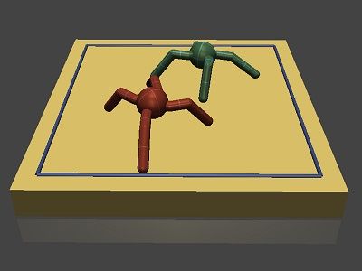
5.4 ROBO S UMO A NTS
Our last experiment is based on the RoboSumo simulation environment in Al-Shedivat et al. (2018)
and Bansal et al. (2017), where two Ants wrestle in an arena. This setting is particularly relevant to
practical robotics research, as we believe success in this simulation could be transferred into the real-
world. The Ants move simultaneously, trying to force the opponent out of the arena or onto the floor.
The physics simulator is MuJoCo (Todorov et al., 2012). The observation space and action space
are continuous. This game is challenging since it involves a complex continuous control problem
with sparse rewards. Following Al-Shedivat et al. (2018) and Bansal et al. (2017), we utilized PPO
(Schulman et al., 2017) with GAE (Schulman et al., 2016) as the base RL algorithm, and used
a 2-layer fully connected network with width 64 for function approximation. Hyper-parameters
N = 50, mk = 500. In Al-Shedivat et al. (2018), a random past opponent is sampled in self-
play, corresponding to the “Self-play w/ random past” baseline here. The agents are initialized from
imitating the pre-trained agents of Al-Shedivat et al. (2018). We considered n = 4 and n = 8 for
our method. From Fig. 7, we observe again that O URS(n = 4, 8) outperform the baseline methods
by a statistical margin and that our method benefits from a larger population size.
6 C ONCLUSION
We propose a new algorithmic framework for competitive self-play policy optimization inspired by
a perturbation subgradient method for saddle points. Our algorithm provably converges in convex-
concave games and achieves better per-agent sample efficiency in several experiments. In the future,
we hope to study a larger population size (should we have sufficient computing power) and the
possibilities of model-based and off-policy self-play RL under our framework.
8Under review as a conference paper at ICLR 2021
R EFERENCES
Maruan Al-Shedivat, Trapit Bansal, Yura Burda, Ilya Sutskever, Igor Mordatch, and Pieter Abbeel.
Continuous adaptation via meta-learning in nonstationary and competitive environments. In In-
ternational Conference on Learning Representations, 2018. 1, 6, 8
Kenneth Joseph Arrow, Hirofumi Azawa, Leonid Hurwicz, and Hirofumi Uzawa. Studies in linear
and non-linear programming, volume 2. Stanford University Press, 1958. 2, 3, 5, 6
Yu Bai and Chi Jin. Provable self-play algorithms for competitive reinforcement learning. arXiv
preprint arXiv:2002.04017, 2020. 2
Bowen Baker, Ingmar Kanitscheider, Todor Markov, Yi Wu, Glenn Powell, Bob McGrew, and Igor
Mordatch. Emergent tool use from multi-agent autocurricula. In International Conference on
Learning Representations, 2020. 1
Trapit Bansal, Jakub Pachocki, Szymon Sidor, Ilya Sutskever, and Igor Mordatch. Emergent com-
plexity via multi-agent competition. ICLR, 2017. 1, 6, 8
Christopher Berner, Greg Brockman, Brooke Chan, Vicki Cheung, Przemyslaw Debiak, Christy
Dennison, David Farhi, Quirin Fischer, Shariq Hashme, Chris Hesse, et al. Dota 2 with large
scale deep reinforcement learning. arXiv preprint arXiv:1912.06680, 2019. 1
Michael Bowling and Manuela Veloso. Multiagent learning using a variable learning rate. Artificial
Intelligence, 136(2):215–250, 2002. 2
George W Brown. Iterative solution of games by fictitious play. Activity analysis of production and
allocation, 13(1):374–376, 1951. 2, 6
Noam Brown and Tuomas Sandholm. Superhuman ai for multiplayer poker. Science, 365(6456):
885–890, 2019. 1, 2
Adrian Rivera Cardoso, Jacob Abernethy, He Wang, and Huan Xu. Competing against nash equilib-
ria in adversarially changing zero-sum games. In International Conference on Machine Learning,
pp. 921–930, 2019. 2
Arpad E Elo. The rating of chessplayers, past and present. Arco Pub., 1978. 6
Adam Gleave, Michael Dennis, Cody Wild, Neel Kant, Sergey Levine, and Stuart Russell. Adver-
sarial policies: Attacking deep reinforcement learning. In International Conference on Learning
Representations, 2019. 3
Jean-Bastien Grill, Florent Altché, Yunhao Tang, Thomas Hubert, Michal Valko, Ioannis
Antonoglou, and Rémi Munos. Monte-carlo tree search as regularized policy optimization. ICML,
2020. 3
Jihun Hamm and Yung-Kyun Noh. K-beam minimax: Efficient optimization for deep adversarial
learning. ICML, 2018. 3
He He, Jordan Boyd-Graber, Kevin Kwok, and Hal Daumé III. Opponent modeling in deep rein-
forcement learning. ICML, 2016. 6
Johannes Heinrich and David Silver. Deep reinforcement learning from self-play in imperfect-
information games. arXiv:1603.01121, 2016. 2, 3
Geoffrey Hinton, Nitish Srivastava, and Kevin Swersky. Neural networks for machine learning
lecture 6a overview of mini-batch gradient descent. 5, 6, 8
Junling Hu and Michael P Wellman. Nash q-learning for general-sum stochastic games. JMLR, 4
(Nov):1039–1069, 2003. 2
M Jaderberg, WM Czarnecki, I Dunning, L Marris, G Lever, AG Castaneda, C Beattie, NC Rabi-
nowitz, AS Morcos, A Ruderman, et al. Human-level performance in 3d multiplayer games with
population-based reinforcement learning. Science, 364(6443):859–865, 2019. 1
9Under review as a conference paper at ICLR 2021
Amir Jafari, Amy Greenwald, David Gondek, and Gunes Ercal. On no-regret learning, fictitious
play, and nash equilibrium. ICML, 2001. 2, 3
MJ Kallio and Andrzej Ruszczynski. Perturbation methods for saddle point computation. 1994. 2,
3, 4, 5, 16
GM Korpelevich. The extragradient method for finding saddle points and other problems. Matecon,
12:747–756, 1976. 2, 3, 4
Marc Lanctot, Vinicius Zambaldi, Audrunas Gruslys, Angeliki Lazaridou, Karl Tuyls, Julien
Pérolat, David Silver, and Thore Graepel. A unified game-theoretic approach to multiagent rein-
forcement learning. In Advances in neural information processing systems, pp. 4190–4203, 2017.
2
Chung-Wei Lee, Haipeng Luo, Chen-Yu Wei, and Mengxiao Zhang. Linear last-iterate convergence
for matrix games and stochastic games. arXiv preprint arXiv:2006.09517, 2020. 2
Michael L Littman. Markov games as a framework for multi-agent reinforcement learning. In
Machine Learning, pp. 157–163. Elsevier, 1994. 2, 6
Siqi Liu, Guy Lever, Josh Merel, Saran Tunyasuvunakool, Nicolas Heess, and Thore Graepel. Emer-
gent coordination through competition. ICLR, 2019. 1
Panayotis Mertikopoulos, Houssam Zenati, Bruno Lecouat, Chuan-Sheng Foo, Vijay Chan-
drasekhar, and Georgios Piliouras. Optimistic mirror descent in saddle-point problems: Going
the extra (gradient) mile. ICLR, 2019. 3, 4, 6
Volodymyr Mnih, Adria Puigdomenech Badia, Mehdi Mirza, Alex Graves, Timothy Lillicrap, Tim
Harley, David Silver, and Koray Kavukcuoglu. Asynchronous methods for deep reinforcement
learning. In ICML, pp. 1928–1937, 2016. 6, 8
John Nash. Non-cooperative games. Annals of mathematics, pp. 286–295, 1951. 2
Angelia Nedić and Asuman Ozdaglar. Subgradient methods for saddle-point problems. Journal of
optimization theory and applications, 2009. 2, 3, 4
Ann Nowé, Peter Vrancx, and Yann-Michaël De Hauwere. Game theory and multi-agent reinforce-
ment learning. Reinforcement Learning, pp. 441, 2012. 2
Manish Prajapat, Kamyar Azizzadenesheli, Alexander Liniger, Yisong Yue, and Anima Anandku-
mar. Competitive policy optimization. arXiv preprint arXiv:2006.10611, 2020. 3
Sasha Rakhlin and Karthik Sridharan. Optimization, learning, and games with predictable se-
quences. In Advances in Neural Information Processing Systems, pp. 3066–3074, 2013. 3
John Schulman, Philipp Moritz, Sergey Levine, et al. High-dimensional continuous control using
generalized advantage estimation. ICLR, 2016. 6, 8
John Schulman, Filip Wolski, Prafulla Dhariwal, Alec Radford, and Oleg Klimov. Proximal policy
optimization algorithms. arXiv preprint arXiv:1707.06347, 2017. 5, 8
Lloyd S Shapley. Stochastic games. PNAS, 39(10):1095–1100, 1953. 3
David Silver, Aja Huang, Chris J Maddison, Arthur Guez, Laurent Sifre, George Van Den Driessche,
Julian Schrittwieser, Ioannis Antonoglou, Veda Panneershelvam, Marc Lanctot, et al. Mastering
the game of go with deep neural networks and tree search. Nature, 529(7587):484, 2016. 1, 2, 3
David Silver, Julian Schrittwieser, Karen Simonyan, Ioannis Antonoglou, Aja Huang, Arthur Guez,
Thomas Hubert, Lucas Baker, Matthew Lai, Adrian Bolton, et al. Mastering the game of go
without human knowledge. Nature, 550(7676):354, 2017. 1, 2, 6
David Silver, Thomas Hubert, Julian Schrittwieser, Ioannis Antonoglou, Matthew Lai, Arthur Guez,
Marc Lanctot, Laurent Sifre, Dharshan Kumaran, Thore Graepel, et al. A general reinforcement
learning algorithm that masters chess, shogi, and go through self-play. Science, 362(6419):1140–
1144, 2018. 1, 6
10Under review as a conference paper at ICLR 2021
Satinder Singh, Michael Kearns, and Yishay Mansour. Nash convergence of gradient dynamics in
general-sum games. UAI, 2000. 2
Richard Sutton and Andrew Barto. reinforcement learning: an introduction. MIT press, 2018. 2, 5
Gerald Tesauro. Temporal difference learning and td-gammon. Communications of the ACM, 38(3):
58–68, 1995. 2
Emanuel Todorov, Tom Erez, and Yuval Tassa. Mujoco: A physics engine for model-based control.
In 2012 IEEE/RSJ International Conference on Intelligent Robots and Systems, pp. 5026–5033.
IEEE, 2012. 8
Oriol Vinyals, Igor Babuschkin, Wojciech M Czarnecki, Michaël Mathieu, Andrew Dudzik, Juny-
oung Chung, David H Choi, Richard Powell, Timo Ewalds, Petko Georgiev, et al. Grandmaster
level in starcraft ii using multi-agent reinforcement learning. Nature, 575(7782):350–354, 2019.
1
Ronald J Williams. Simple statistical gradient-following algorithms for connectionist reinforcement
learning. Machine learning, 8(3-4):229–256, 1992. 6
Kaiqing Zhang, Sham M Kakade, Tamer Başar, and Lin F Yang. Model-based multi-agent rl in
zero-sum markov games with near-optimal sample complexity. arXiv preprint arXiv:2007.07461,
2020. 2
Martin Zinkevich, Michael Johanson, Michael Bowling, and Carmelo Piccione. Regret minimization
in games with incomplete information. In Advances in neural information processing systems, pp.
1729–1736, 2008. 2, 3
11Under review as a conference paper at ICLR 2021
A E XPERIMENT DETAILS
A.1 I LLUSTRATIONS OF THE GAMES IN THE EXPERIMENTS
Illustration Properties
Fig. 8: Illustration of the 6x9 grid-world Observation space:
soccer game. Red and blue represent the Tensor of shape [5, ],
two teams A and B. At start, the players (xA , yA , xB , yB , A has
are initialized to random positions on re- ball)
spective sides, and the ball is randomly Action space:
A
assigned to one team. Players move up, {up, down, left, right, noop}
B
down, left and right. Once a player scores a Time limit:
goal, the corresponding team wins and the 50 moves
game ends. One player can intercept the Terminal reward:
other’s ball by crossing the other player. +1 for winning team
−1 for losing team
0 if timeout
Fig. 9: Illustration of the Gomoku game Observation space:
(also known as Renju, five-in-a-row). We Tensor of shape [9, 9, 3],
study the 9x9 board variant. Two players last dim 0: vacant, 1:
1 2 3 4 5 6 7 8 9
sequentially place black and white stones black, 2: white
on the board. Black goes first. A player Action space:
8 2 12
wins when he or she gets five stones in a Any valid location on the
13 11 9 1 3 10
7 4 6
row. In the case of this illustration, the 9x9 board
5 black wins because there is five consecu- Time limit:
tive black stones in the 5th row. Numbers 41 moves per-player
A B C D E F G H I
in the stones indicate the ordered they are Terminal reward:
placed. +1 for winning player
−1 for losing player
0 if timeout
Fig. 10: Illustration of the RoboSumo Ants
game. Two ants fight in the arena. The goal
is to push the opponent out of the arena Observation space:
or down to the floor. Agent positions are R120
initialized to be random at the start of the Action space:
game. The game ends in a draw if the time R8
limit is reached. In addition to the terminal Time limit:
±1 reward, the environment comes with 100 moves
shaping rewards (motion bonus, closeness Reward:
to opponent, etc.). In order to make the
game zero-sum, we take the difference be- rt = rtorig y − rtorig x
tween the original rewards of the two ants. Terminal ±1 or 0.
A.2 H YPER - PARAMETERS
The hyper-parameters in different games are listed in Tab. 5.
A.3 A DDITIONAL RESULTS
Win-rates (or average rewards). Here we report additional results in terms of the average win-
rates, or equivalently the average rewards through the linear transform win-rate = 0.5 + 0.5 reward,
in Tab. 6 and 7. Since we treat each (xi , yi ) pair as one agent, the values are the average of f (xi , ·)
and f (·, yi ) in the first table. The one-side f (·, yi ) win-rates are in the second table. Mean and 95%
confidence intervals are estimated from multiple runs. Exact numbers of runs are in the captions
12Under review as a conference paper at ICLR 2021
Tab. 5: Hyper-parameters.
Hyper-param \ Game Soccer Gomoku RoboSumo
Num. of iterations N 50 40 50
0 → 0.001 in first
Learning rate ηk 0.1 3e-5 → 0 linearly
20 steps then 0.001
Value func learning rate (Same as above.) (Same as above.) 9e-5
Sample size mk 32 32 500
Num. of inner updates l 10 10 10
Env. time limit 50 41 per-player 100
PPO, clip 0.2, mini-
Base RL algorithm A2C A2C
batch 512, epochs 3
Optimizer RmsProp, α = 0.99 RmsProp, α = 0.99 RmsProp, α = 0.99
Max gradient norm 1.0 1.0 0.1
GAE λ parameter 0.95 0.95 0.98
Discounting factor γ 0.97 0.97 0.995
Entropy bonus coef. 0.01 0.01 0
Sequential[
Sequential[ Linear[120,64],
Conv[c16,k5,p2], TanH,
ReLU, Linear[64,64],
Sequential[
Conv[c32,k5,p2], TanH,
OneHot[5832],
ReLU, Linear[64,8],
Policy function Linear[5832,5],
Conv[c64,k3,p1], TanH,
Softmax,
ReLU, GaussianDist ]
CategoricalDist ]
Conv[c1,k1], Tanh ensures the mean
Spatial Softmax, of the Gaussian is be-
CategoricalDist ] tween -1 and 1. The
density is corrected.
Sequential[
Share 3 Conv layers
Linear[120,64],
Sequential[ with the policy, but
TanH,
Value function OneHot[5832], additional heads:
Linear[64,64],
Linear[5832,1] ] global average and
TanH,
Linear[64,1]
Linear[64,1] ]
13Under review as a conference paper at ICLR 2021
of Fig. 5,6,7 of the main paper. The message is the same as that suggested by the Elo scores: Our
method consistently produces stronger agents. We hope the win-rates may give better intuition about
the relative performance of different methods.
Tab. 6: Average win-rates (∈ [0, 1]) between the last-iterate (final) agents trained by different algo-
rithms. Last two rows further show the average over other last-iterate agents and all other agents
(historical checkpoint) included in the tournament, respectively. Since an agent consists of an (x, y)
row col
(xcol ,y row )
pair, the win-rate is averaged on x and y, i.e., win(col vs row) = f (x ,y )−f 2 × 0.5 + 0.5.
The lower the better within each column; The higher the better within each row.
(a) Soccer
Soccer Self-play latest Self-play best Self-play rand Ours (n=2) Ours (n=4) Ours (n=6)
Self-play latest - 0.533 ± 0.044 0.382 ± 0.082 0.662 ± 0.054 0.691 ± 0.029 0.713 ± 0.032
Self-play best 0.467 ± 0.044 - 0.293 ± 0.059 0.582 ± 0.042 0.618 ± 0.031 0.661 ± 0.030
Self-play rand 0.618 ± 0.082 0.707 ± 0.059 - 0.808 ± 0.039 0.838 ± 0.028 0.844 ± 0.043
Ours (n=2) 0.338 ± 0.054 0.418 ± 0.042 0.192 ± 0.039 - 0.549 ± 0.022 0.535 ± 0.022
Ours (n=4) 0.309 ± 0.029 0.382 ± 0.031 0.162 ± 0.028 0.451 ± 0.022 - 0.495 ± 0.023
Ours (n=6) 0.287 ± 0.032 0.339 ± 0.030 0.156 ± 0.043 0.465 ± 0.022 0.505 ± 0.023 -
Last-iter average 0.357 ± 0.028 0.428 ± 0.028 0.202 ± 0.023 0.532 ± 0.023 0.608 ± 0.018 0.585 ± 0.022
Overall average 0.632 ± 0.017 0.676 ± 0.014 0.506 ± 0.020 0.749 ± 0.009 0.775 ± 0.006 0.776 ± 0.008
(b) Gomoku
Gomoku Self-play latest Self-play best Self-play rand Ours (n=2) Ours (n=4) Ours (n=6)
Self-play latest - 0.523 ± 0.026 0.462 ± 0.032 0.551 ± 0.024 0.571 ± 0.018 0.576 ± 0.017
Self-play best 0.477 ± 0.026 - 0.433 ± 0.031 0.532 ± 0.024 0.551 ± 0.018 0.560 ± 0.020
Self-play rand 0.538 ± 0.032 0.567 ± 0.031 - 0.599 ± 0.027 0.588 ± 0.022 0.638 ± 0.020
Ours (n=2) 0.449 ± 0.024 0.468 ± 0.024 0.401 ± 0.027 - 0.528 ± 0.015 0.545 ± 0.017
Ours (n=4) 0.429 ± 0.018 0.449 ± 0.018 0.412 ± 0.022 0.472 ± 0.015 - 0.512 ± 0.013
Ours (n=6) 0.424 ± 0.017 0.440 ± 0.020 0.362 ± 0.020 0.455 ± 0.017 0.488 ± 0.013 -
Last-iter average 0.455 ± 0.010 0.479 ± 0.011 0.407 ± 0.012 0.509 ± 0.010 0.537 ± 0.008 0.560 ± 0.008
Overall average 0.541 ± 0.004 0.561 ± 0.004 0.499 ± 0.005 0.583 ± 0.004 0.599 ± 0.003 0.615 ± 0.003
(c) RoboSumo
RoboSumo Self-play latest Self-play best Self-play rand Ours (n=4) Ours (n=8)
Self-play latest - 0.502 ± 0.012 0.493 ± 0.013 0.511 ± 0.011 0.510 ± 0.010
Self-play best 0.498 ± 0.012 - 0.506 ± 0.014 0.514 ± 0.008 0.512 ± 0.010
Self-play rand 0.507 ± 0.013 0.494 ± 0.014 - 0.508 ± 0.011 0.515 ± 0.011
Ours (n=4) 0.489 ± 0.011 0.486 ± 0.008 0.492 ± 0.011 - 0.516 ± 0.008
Ours (n=8) 0.490 ± 0.010 0.488 ± 0.010 0.485 ± 0.011 0.484 ± 0.008 -
Last-iter average 0.494 ± 0.006 0.491 ± 0.005 0.492 ± 0.006 0.500 ± 0.005 0.514 ± 0.005
Overall average 0.531 ± 0.004 0.527 ± 0.004 0.530 ± 0.004 0.539 ± 0.003 0.545 ± 0.003
Training time. Thanks to the easiness of parallelization, the proposed algorithm enjoys good scal-
ability. We can either distribute the n agents into n processes to run concurrently, or make the roll-
outs parallel. Our implementation took the later approach. In the most time-consuming RoboSumo
Ants experiment, with 30 Intel Xeon CPUs, the baseline methods took approximately 2.4h, while
Ours (n=4) took 10.83h to train (×4.5 times), and Ours (n=8) took 20.75h (×8.6 times). Note that,
Ours (n) trains n agents simultaneously. If we train n agents with the baseline methods by repeating
the experiment n times, the time would be 2.4n hours, which is comparable to Ours (n).
Chance of selecting the agent itself as opponent. One big difference between our method and the
compared baselines is the ability to select opponents adversarially from the population. Consider the
agent pair (xi , yi ). When training xi , our method finds the strongest opponent (that incurs the largest
loss on xi ) from the population, whereas the baselines always choose (possibly past versions of) yi .
Since the candidate set contains yi , the “fall-back” case is to use yi as opponent in our method. We
report the frequency that yi is chosen as opponent for xi (and xi for yi likewise). This gives a sense
of how often our method falls back to the baseline method. From Tab. 8, we can observe that, as n
grows larger, the chance of fall-back is decreased. This is understandable since a larger population
means larger candidate sets and a larger chance to find good perturbations.
B P ROOFS
We adopt the following variant of Alg. 1 in our asymptotic convergence analysis. For clarity, we
investigate the learning process of one agent in the population and drop the i index. Cxk and Cyk are
14Under review as a conference paper at ICLR 2021
Tab. 7: Average one-sided win-rates (∈ [0, 1]) between the last-iterate (final) agents trained by
different algorithms. The win-rate is one-sided, i.e., win(y col vs xrow ) = f (xrow , y col ) × 0.5 + 0.5.
The lower the better within each column; The higher the better within each row.
(a) Soccer
row x \ col y Self-play latest Self-play best Self-play rand Ours (n=2) Ours (n=4) Ours (n=6)
Self-play latest 0.536 ± 0.054 0.564 ± 0.079 0.378 ± 0.103 0.674 ± 0.080 0.728 ± 0.039 0.733 ± 0.048
Self-play best 0.497 ± 0.065 0.450 ± 0.064 0.306 ± 0.106 0.583 ± 0.056 0.601 ± 0.039 0.642 ± 0.050
Self-play rand 0.614 ± 0.163 0.719 ± 0.090 0.481 ± 0.102 0.796 ± 0.071 0.816 ± 0.039 0.824 ± 0.062
Ours (n=2) 0.350 ± 0.051 0.419 ± 0.057 0.181 ± 0.049 0.451 ± 0.037 0.525 ± 0.031 0.553 ± 0.034
Ours (n=4) 0.346 ± 0.046 0.365 ± 0.047 0.140 ± 0.034 0.427 ± 0.034 0.491 ± 0.020 0.494 ± 0.033
Ours (n=6) 0.308 ± 0.042 0.319 ± 0.052 0.136 ± 0.050 0.483 ± 0.043 0.505 ± 0.030 0.515 ± 0.032
Last-iter average 0.381 ± 0.033 0.422 ± 0.036 0.188 ± 0.028 0.525 ± 0.029 0.601 ± 0.021 0.587 ± 0.026
Overall average 0.654 ± 0.017 0.665 ± 0.016 0.502 ± 0.021 0.745 ± 0.010 0.771 ± 0.006 0.775 ± 0.009
(b) Gomoku
row x \ col y Self-play latest Self-play best Self-play rand Ours (n=2) Ours (n=4) Ours (n=6)
Self-play latest 0.481 ± 0.031 0.540 ± 0.038 0.488 ± 0.050 0.594 ± 0.041 0.571 ± 0.026 0.586 ± 0.030
Self-play best 0.494 ± 0.033 0.531 ± 0.030 0.471 ± 0.049 0.597 ± 0.040 0.562 ± 0.024 0.572 ± 0.028
Self-play rand 0.565 ± 0.036 0.605 ± 0.036 0.572 ± 0.051 0.668 ± 0.040 0.617 ± 0.027 0.647 ± 0.029
Ours (n=2) 0.491 ± 0.031 0.533 ± 0.033 0.470 ± 0.040 0.568 ± 0.035 0.571 ± 0.022 0.552 ± 0.025
Ours (n=4) 0.428 ± 0.022 0.461 ± 0.024 0.440 ± 0.035 0.515 ± 0.029 0.491 ± 0.017 0.503 ± 0.020
Ours (n=6) 0.435 ± 0.021 0.453 ± 0.026 0.370 ± 0.028 0.462 ± 0.025 0.479 ± 0.018 0.467 ± 0.017
Last-iter average 0.472 ± 0.012 0.506 ± 0.014 0.438 ± 0.017 0.549 ± 0.016 0.550 ± 0.011 0.564 ± 0.012
Overall average 0.548 ± 0.005 0.585 ± 0.005 0.536 ± 0.007 0.631 ± 0.006 0.608 ± 0.004 0.617 ± 0.004
(c) RoboSumo
row x \ col y Self-play latest Self-play best Self-play rand Ours (n=4) Ours (n=8)
Self-play latest 0.516 ± 0.022 0.494 ± 0.020 0.491 ± 0.023 0.502 ± 0.017 0.511 ± 0.016
Self-play best 0.489 ± 0.018 0.504 ± 0.023 0.503 ± 0.022 0.506 ± 0.014 0.509 ± 0.014
Self-play rand 0.505 ± 0.021 0.491 ± 0.026 0.494 ± 0.026 0.518 ± 0.017 0.516 ± 0.014
Ours (n=4) 0.480 ± 0.018 0.479 ± 0.012 0.502 ± 0.016 0.496 ± 0.009 0.517 ± 0.012
Ours (n=8) 0.491 ± 0.012 0.484 ± 0.016 0.485 ± 0.016 0.486 ± 0.012 0.491 ± 0.012
Last-iter average 0.489 ± 0.008 0.485 ± 0.008 0.495 ± 0.009 0.500 ± 0.007 0.514 ± 0.007
Overall average 0.528 ± 0.004 0.521 ± 0.004 0.530 ± 0.005 0.534 ± 0.003 0.544 ± 0.003
Tab. 8: Average frequency of using the agent itself as opponent, in the Soccer and Gomoku exper-
iments. The frequency is calculated by counting over all agents and iterations. The ± shows the
standard deviations estimated by 3 runs with different random seeds.
Method Ours (n = 2) Ours (n = 4) Ours (n = 6)
Frequency of self (Soccer) 0.4983 ± 0.0085 0.2533 ± 0.0072 0.1650 ± 0.0082
Frequency of self (Gomoku) 0.5063 ± 0.0153 0.2312 ± 0.0111 0.1549 ± 0.0103
not set simply as the population for the sake of the proof. Alternatively, we pose some assumptions.
Setting them to the population as in the main text may approximately satisfy the assumptions.
Algorithm 2: Simplified perturbation-based self-play policy optimization of one agent.
Input: ηk : learning rates, mk : sample size;
Result: Pair of policies (x, y);
1 Initialize x0 , y 0 ;
2 for k = 0, 1, 2, . . . ∞ do
3 Construct candidate opponent sets Cyk and Cxk ;
4 Find perturbed v k = arg maxy∈Cyk fˆ(xk , y) and perturbed uk = arg minx∈Cxk fˆ(x, y k ) where the
evaluation is done with Eq. 4 and sample size mk ;
5 Compute estimated duality gap Êk = fˆ(xk , v k ) − fˆ(uk , y k );
6 if Êk ≤ 3 then
7 return (xk , y k )
8 ˆ x f (xk , v k ) and ĝyk = ∇
Estimate policy gradients ĝxk = ∇ ˆ y f (uk , y k ) w/ Eq. 5 and sample size mk ;
9 Update policy parameters with xk+1 ← xk − ηk ĝxk and y k+1 ← y k + ηk ĝyk ;
B.1 P ROOF OF T HEOREM 1
We restate the assumptions and the theorem here more clearly for reference.
15You can also read