Embedding of FRPN in CNN architecture - ESANN 2020
←
→
Page content transcription
If your browser does not render page correctly, please read the page content below
ESANN 2020 proceedings, European Symposium on Artificial Neural Networks, Computational Intelligence
and Machine Learning. Online event, 2-4 October 2020, i6doc.com publ., ISBN 978-2-87587-074-2.
Available from http://www.i6doc.com/en/.

            Embedding of FRPN in CNN architecture
       Alberto Rossi1 and Markus Hagenbuchner2 and Franco Scarselli3 and Ah Chung Tsoi2

                   1- Department of Information Engineering - University of Florence
                              Via di S. Marta 3, 50139 Firenze - Italy
           2- School of Computing and Information Technology - University of Wollongong
                          Northfields Avenue, 2522 Wollongong - Australia
                    3- Department of Information Engineering - University of Siena
                                  Via Roma 56, 53100 Siena - Italy

            Abstract. This paper extends the fully recursive perceptron network
            (FRPN) model for vectorial inputs to include deep convolutional neural
            networks (CNNs) which can accept multi-dimensional inputs. A FRPN
            consists of a recursive layer, which, given a fixed input, iteratively com-
            putes an equilibrium state. The unfolding realized with this kind of itera-
            tive mechanism allows to simulate a deep neural network with any number
            of layers. The extension of the FRPN to CNN results in an architecture,
            which we call convolutional-FRPN (C-FRPN), where the convolutional
            layers are recursive. The method is evaluated on several image classifica-
            tion benchmarks. It is shown that the C-FRPN consistently outperforms
            standard CNNs having the same number of parameters. The gap in perfor-
            mance is particularly large for small networks, showing that the C-FRPN
            is a very powerful architecture, since it allows to obtain equivalent perfor-
            mance with fewer parameters when compared with deep CNNs.

      1    Introduction
      Convolutional Neural Networks (CNNs) emerged in the last decade as a leading
      method to process images [1, 2]. Modern CNNs have deep and wide-width
      architectures [2]. One of the first CNNs [1] was composed of five layers, two of
      which were convolutional. The depth of the models in subsequent years showed a
      continuously increasing trend. The AlexNet [3] and the ZFNet [4] architectures,
      which won the object recognition task at ILSRVC in 2012 and 2013, respectively,
      have 8 layers. GoogLeNet, the winning model at ILSRVC [5] in 2014, is a CNN
      composed of 22 layers. A major advance in performance was obtained in the
      following year by ResNet [6], based on a highway network architecture, consisting
      of 152 layers. Such a relationship between the increase in performance level and
      the depth of the network was observed in many other image related tasks, e.g.,
      object detection, semantic segmentation, image generation [7, 8, 9, 10].
          Despite the important role played by the depth of the architectures, such
      a meta–parameter is still chosen by heuristics and by a trial and error pro-
      cess. Moreover, the depth, once determined, remains fixed during the learning
      and application phase and for each input exemplar class. In order to overcome
      these limitations, in this paper, we extend the fully recursive perceptron network
      (FRPN) [11] to include CNNs. The FRPN is an architecture in which all the
      hidden neurons are fully connected with a weight parameters [11]. Intuitively,

                                                 133
ESANN 2020 proceedings, European Symposium on Artificial Neural Networks, Computational Intelligence
and Machine Learning. Online event, 2-4 October 2020, i6doc.com publ., ISBN 978-2-87587-074-2.
Available from http://www.i6doc.com/en/.
the hidden layer of a FRPN implements a recursive layer, that, given a fixed
input, iteratively computes a hidden state until the state itself converges [11].
The extended model, which we call a convolutional-FRPN (C-FRPN), is
characterized by convolutional layers having weighted parameter feedback con-
nections. In those layers, the convolutions are applied on the concatenation of
the output of the convolutions at the previous iteration with the static input
coming from the previous layer, realizing a kind of state iteration on feature
maps. The computation evolves until the feature maps converge. In this way,
the unfolding of a C-FRPN is a deep network, where the number of layers is
not fixed, but adapted automatically to suit a given task or to suit a particular
input sample.
The proposed architecture is related to recurrent convolutional neural net-
works (RCNNs) [12], which use recurrent layers, and reported very good results
on several image classification tasks. However, in RCNNs, the number of iter-
ations is predefined and thus the unfolded architecture is of a fixed depth, and
requires a manually defined hyper-parameter for each recursive layer, whereas
in C-FRPN such a parameter is learned.
This paper studies the effectiveness of the proposed method via experimen-
tation on standard natural image benchmark datasets (CIFAR-10 and SVHN),
and on a real-world problem on melanoma prediction (the ISIC dataset). The
experiments revealed that C-FRPNs outperform CNNs having the same number
of weight parameters. The difference is particularly evident for smaller archi-
tectures where the number of weights is small. Those results suggest that the
C-FRPN model is more powerful in terms of approximation capability than the
standard CNN with the same number of parameters. Such a capability is easy to
be exploited if a sufficient number of training examples is available, and allows
to solve a problem with applications where computational resources are limited.
The rest of the paper is organized as follows: Section 2 recalls the FRPN
model, Section 3 introduces the C–FRPN architecture, Section 4 describes the
used datasets, the experimental settings and the obtained results. Finally, Sec-
tion 5 offers concluding remarks.
2 The FRPN model
A FRPN is a neural network with an input layer, a single hidden layer and an
output layer. The peculiarity of a FRPN is the hidden layer, the neurons of
which are fully connected with the other, including with themselves, and to the
inputs via links with unknown weights. Formally, if u = [u1 , . . . , um ] is an input
vector and x(t) = [x1 (t), . . . , xn (t)] is the output of the hidden layer at time t,
then m n
X X
xi (t) = f ( αij uj + βik xk (t − 1) + bi ) (1)
j=1 k=1
where bi are bias weights, αij are the input to hidden connection weights, and
βik are the hidden to hidden connection weights, for i = 1, 2, ..., n, j = 1, 2, ..., m
and k = 1, 2, ..., n.
134ESANN 2020 proceedings, European Symposium on Artificial Neural Networks, Computational Intelligence
and Machine Learning. Online event, 2-4 October 2020, i6doc.com publ., ISBN 978-2-87587-074-2.
Available from http://www.i6doc.com/en/.
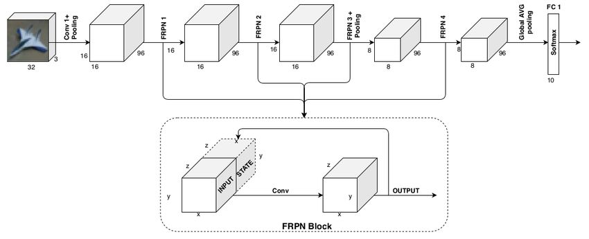
Fig. 1: The C-FRPN architecture. On top the whole network constituted by 4
C-FRPN layers. On bottom, a C-FRPN layer.
Equation (1) defines a dynamic System. In order to calculate the outputs of
the hidden neurons, the computation in Equation (1) is iterated until the state x
converges to a stable point or until a maximum number of iterations is reached.
In practice, this allows to unfold the network for a number of iterations that
is not pre-defined, but it depends on the “richness” of the input1 . Moreover,
the shared weights in the unfolding network give an opportunity to have a deep
network architecture, requiring a small number of weights. Indeed, in [11] it
is formally shown that any deep multi-layer feedforward neural network can be
simulated by an FRPN, and predicts advantages of the latter model (FRPN)
over the former (deep CNN) in terms of approximation capabilities.
3 C-FRPN
A C-FRPN architecture (top of Fig. 1) consists of a CNN in which the convolu-
tional layers are C-FRPN layers. Each C-FRPN layer computes a set of feature
maps taking in input a stack of the feature maps provided by the previous layer
and the feature maps of the same layer at the previous time step (bottom of
Fig. 1). C-FRPN layers behave as FRPNs, where the feature maps, which cor-
respond to the state, are iteratively computed until they reach a stable point.
As in conventional CNN, a C-FRPN layer may be followed by dropout and/or
batch normalization layers. Moreover, the architecture may include at the end
some full connected layers as is illustrated in Fig. 1.
This architecture is similar to the RCNN proposed in [12]. The RCNN con-
sists of 4 layers and each of these unfold exactly 3 times. At each iteration each
layer takes always the same input concatenated with the output evaluated at the
previous time step. The RCNN produced interesting results on three different
datasets, proving the benefits of this kind of network.
1 A “rich” input excites the latent modes in the system and would characterize the behaviour
of the underlying system. This is an essential assumption in any system identification study.
135ESANN 2020 proceedings, European Symposium on Artificial Neural Networks, Computational Intelligence
and Machine Learning. Online event, 2-4 October 2020, i6doc.com publ., ISBN 978-2-87587-074-2.
Available from http://www.i6doc.com/en/.
The first novelty of our approach regards the possibility for each layer to
evolve until the state converges to a stable point. This means that the recursive
layers are not constrained to unfold for a fixed number of times and such a
hyper-parameter has not to be manually set. Furthermore, we obtain a variable
depth network: to the best of our knowledge this is the first time that such
an architecture is proposed for CNNs. Another improvement resides in the
experimentation carried out that allows to compare the performance of C-FRPN
and CNN and disclose interesting differences in their behaviour.
4 Experimentation
Experiments have been carried out on three datasets: CIFAR-10 [13], SVHN [14]
and ISIC [15]. We used a C-FRPN having the overall structure as the one
deployed in [12]. The C-FRPN was compared with a baseline CNN having
the same number of layers and the same number of unknown parameters. The
architecture included 4 convolutional layers with ReLu activation function and
the same number of feature maps on all layers: 6 different experiments have been
run, where the feature maps were [135, 120, 104, 85, 42, 21] for the baseline CNN
and [96, 85, 74, 60, 30, 15] for the C-FRPN, respectively. The kernel size of the
first convolution is 5×5 with stride 1, while for the remaining convolutional layers
are 3×3 with stride 1. Each C-FRPN layer was followed by a pooling layer of size
3 × 3 and stride 2. Moreover, we added a local response normalization operation
after each iteration of the C-FRPN layer and a dropout layer with a forget rate
of 0.5 after each convolution except the last one. The state convergence was
evaluated by means of the Euclidean distance between the current state and
the previous one: the state was considered converged when the distance was
smaller than 0.1 or a maximum number of 8 iterations was reached2 . The image
augmentation method in [12] was deployed for CIFAR-10 and SVHN, while for
ISIC, we used random horizontal and vertical flips, and random rotations. The
Adam optimizer was used with learning rate 1 × 10⁻⁴ , weight decay 5 × 10⁻⁴ ,
and, batch size 128 for CIFAR-10 and SVHN, and 24 for ISIC. The experiments
were repeated 5 times by using different random initial conditions.
Fig. 2 summarizes the results. The figure reveals that the C-FRPN achieves
a higher accuracy when compared with a baseline having the same architecture
and the same number of parameters. The difference is more evident for smaller
networks. Fig. 3 analyses the validation performance of a single run on the SVHN
dataset. It can be observed that the C-FRPN performance is better throughout
a training session and that such improvement is more evident for smaller net-
works. The results suggest that the C-FRPN model is more powerful in terms
of approximation capability than the standard CNN. Such a capability can fa-
cilitate applications with constraints in computational power and corresponding
memory load.
2 A maximum number of iterations has to be set both for computational reasons and because
the convergence cannot be guaranteed without further considerations.
136ESANN 2020 proceedings, European Symposium on Artificial Neural Networks, Computational Intelligence
and Machine Learning. Online event, 2-4 October 2020, i6doc.com publ., ISBN 978-2-87587-074-2.
Available from http://www.i6doc.com/en/.
CIFAR-10 SVHN ISIC
90
96 82
85 94 81
80 92 80
Accuracy
Accuracy
Accuracy
79
75 90
78
70 88
77
65 86
Model Model 76 Model
Baseline Baseline Baseline
FRPN 84 FRPN 75 FRPN
60
672K 527K 400K 264K 67K 17K 672K 527K 400K 264K 67K 17K 672K 527K 400K 264K 67K 17K
Network Size Network Size Network Size
Fig. 2: A box plot of accuracies achieved by C-FRPN and the baseline.
Number of weights=672K Number of weights=572K Number of weights=400K
95
90
Accuracy (%)
85
80
75 Baseline Baseline Baseline
FRPN FRPN FRPN
70
Number of weights=264K Number of weights=67K Number of weights=17K
95 Baseline
FRPN
90
Accuracy (%)
85
80
75 Baseline Baseline
FRPN FRPN
70
0 100 200 300 400 500 0 100 200 300 400 500 0 100 200 300 400 500
Epoch Epoch Epoch
Fig. 3: The validation performance of C-FRPN and the baseline CNN during
learning the SVHN data.
5 Conclusion
This paper proposed the C-FRPN model, which can be considered a general-
ization of both the FRPN [11] and the RCNN [12] architectures. The C-FRPN
model realizes variable depth CNNs. An experimental evaluation revealed con-
sistent advantages of the novel architecture, particularly for a small number of
parameters. As matters of future research, a more extensive set of experiments
and a deeper study of the role played by each C-FRPN layer in the architec-
ture would be most beneficial in understanding the capabilities of this novel
137ESANN 2020 proceedings, European Symposium on Artificial Neural Networks, Computational Intelligence
and Machine Learning. Online event, 2-4 October 2020, i6doc.com publ., ISBN 978-2-87587-074-2.
Available from http://www.i6doc.com/en/.
architecture.
References
[1] Yann LeCun, Léon Bottou, Yoshua Bengio, Patrick Haffner, et al. Gradient-based learning
applied to document recognition. Proceedings of the IEEE, 86(11):2278–2324, 1998.
[2] Md Zahangir Alom, Tarek M. Taha, Chris Yakopcic, Stefan Westberg, Paheding Sidike,
Mst Shamima Nasrin, Mahmudul Hasan, Brian C. Van Essen, Abdul A. S. Awwal, and
Vijayan K. Asari. A state-of-the-art survey on deep learning theory and architectures.
Electronics, 8(3), 2019.
[3] Alex Krizhevsky, Ilya Sutskever, and Geoffrey E Hinton. Imagenet classification with deep
convolutional neural networks. In Advances in neural information processing systems,
pages 1097–1105, 2012.
[4] Matthew D Zeiler and Rob Fergus. Visualizing and understanding convolutional networks.
In European conference on computer vision, pages 818–833. Springer, 2014.
[5] Christian Szegedy, Wei Liu, Yangqing Jia, Pierre Sermanet, Scott Reed, Dragomir
Anguelov, Dumitru Erhan, Vincent Vanhoucke, and Andrew Rabinovich. Going deeper
with convolutions. In Proceedings of the IEEE conference on computer vision and pattern
recognition, pages 1–9, 2015.
[6] Kaiming He, Xiangyu Zhang, Shaoqing Ren, and Jian Sun. Deep residual learning for
image recognition. In Proceedings of the IEEE conference on computer vision and pattern
recognition, pages 770–778, 2016.
[7] Joseph Redmon, Santosh Divvala, Ross Girshick, and Ali Farhadi. You only look once:
Unified, real-time object detection. In Proceedings of the IEEE conference on computer
vision and pattern recognition, pages 779–788, 2016.
[8] Liang-Chieh Chen, George Papandreou, Iasonas Kokkinos, Kevin Murphy, and Alan L
Yuille. Deeplab: Semantic image segmentation with deep convolutional nets, atrous con-
volution, and fully connected crfs. IEEE transactions on pattern analysis and machine
intelligence, 40(4):834–848, 2017.
[9] Phillip Isola, Jun-Yan Zhu, Tinghui Zhou, and Alexei A Efros. Image-to-image translation
with conditional adversarial networks. In Proceedings of the IEEE conference on computer
vision and pattern recognition, pages 1125–1134, 2017.
[10] Paolo Andreini, Simone Bonechi, Monica Bianchini, Alessandro Mecocci, Franco Scarselli,
and Andrea Sodi. A two stage gan for high resolution retinal image generation and
segmentation. arXiv preprint arXiv:1907.12296, 2019.
[11] Markus Hagenbuchner, Ah Chung Tsoi, Franco Scarselli, and Shu Jia Zhang. A fully
recursive perceptron network architecture. In 2017 IEEE Symposium Series on Compu-
tational Intelligence (SSCI), pages 1–8. IEEE, 2017.
[12] Ming Liang and Xiaolin Hu. Recurrent convolutional neural network for object recogni-
tion. In Proceedings of the IEEE conference on computer vision and pattern recognition,
pages 3367–3375, 2015.
[13] Alex Krizhevsky, Geoffrey Hinton, et al. Learning multiple layers of features from tiny
images. Technical report, Citeseer, 2009.
[14] Yuval Netzer, Tao Wang, Adam Coates, Alessandro Bissacco, Bo Wu, and Andrew Y Ng.
Reading digits in natural images with unsupervised feature learning. 2011.
[15] Noel CF Codella, David Gutman, M Emre Celebi, Brian Helba, Michael A Marchetti,
Stephen W Dusza, Aadi Kalloo, Konstantinos Liopyris, Nabin Mishra, Harald Kittler,
et al. Skin lesion analysis toward melanoma detection: A challenge at the 2017 interna-
tional symposium on biomedical imaging (isbi), hosted by the international skin imaging
collaboration (isic). In 2018 IEEE 15th International Symposium on Biomedical Imaging
(ISBI 2018), pages 168–172. IEEE, 2018.
138You can also read