Emergent Complexity and Zero-shot Transfer via Unsupervised Environment Design - arXiv.org
←
→
Page content transcription
If your browser does not render page correctly, please read the page content below
Emergent Complexity and Zero-shot Transfer via
                                                      Unsupervised Environment Design

                                                       Michael Dennis∗, Natasha Jaques∗2 , Eugene Vinitsky, Alexandre Bayen,
                                                                     Stuart Russell, Andrew Critch, Sergey Levine
                                                       University of California Berkeley AI Research (BAIR), Berkeley, CA, 94704
                                                               2
                                                                 Google Research, Brain team, Mountain View, CA, 94043
arXiv:2012.02096v2 [cs.LG] 4 Feb 2021

                                                         michael_dennis@berkeley.edu, natashajaques@google.com,
                                                       @berkeley.edu

                                                                                        Abstract
                                                     A wide range of reinforcement learning (RL) problems — including robustness,
                                                     transfer learning, unsupervised RL, and emergent complexity — require speci-
                                                     fying a distribution of tasks or environments in which a policy will be trained.
                                                     However, creating a useful distribution of environments is error prone, and takes
                                                     a significant amount of developer time and effort. We propose Unsupervised
                                                     Environment Design (UED) as an alternative paradigm, where developers pro-
                                                     vide environments with unknown parameters, and these parameters are used to
                                                     automatically produce a distribution over valid, solvable environments. Existing
                                                     approaches to automatically generating environments suffer from common failure
                                                     modes: domain randomization cannot generate structure or adapt the difficulty of
                                                     the environment to the agent’s learning progress, and minimax adversarial training
                                                     leads to worst-case environments that are often unsolvable. To generate struc-
                                                     tured, solvable environments for our protagonist agent, we introduce a second,
                                                     antagonist agent that is allied with the environment-generating adversary. The
                                                     adversary is motivated to generate environments which maximize regret, defined as
                                                     the difference between the protagonist and antagonist agent’s return. We call our
                                                     technique Protagonist Antagonist Induced Regret Environment Design (PAIRED).
                                                     Our experiments demonstrate that PAIRED produces a natural curriculum of in-
                                                     creasingly complex environments, and PAIRED agents achieve higher zero-shot
                                                     transfer performance when tested in highly novel environments.

                                        1       Introduction
                                        Many reinforcement learning problems require designing a distribution of tasks and environments
                                        that can be used to evaluate and train effective policies. This is true for a diverse array of methods
                                        including transfer learning (e.g., [2, 50, 34, 43]), robust RL (e.g., [4, 16, 30]), unsupervised RL (e.g.,
                                        [15]), and emergent complexity (e.g., [40, 47, 48]). For example, suppose we wish to train a robot
                                        in simulation to pick up objects from a bin in a real-world warehouse. There are many possible
                                        configurations of objects, including objects being stacked on top of each other. We may not know a
                                        priori the typical arrangement of the objects, but can naturally describe the simulated environment as
                                        having a distribution over the object positions.
                                        However, designing an appropriate distribution of environments is challenging. The real world is
                                        complicated, and correctly enumerating all of the edge cases relevant to an application could be
                                        impractical or impossible. Even if the developer of the RL method knew every edge case, specifying
                                        this distribution could take a significant amount of time and effort. We want to automate this process.
                                            ∗
                                                Equal contribution

                                        34th Conference on Neural Information Processing Systems (NeurIPS 2020), Vancouver, Canada.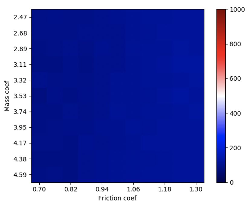
(a) Domain Randomization (b) Minimax Adversarial       (c) PAIRED (ours)        (d) Transfer task
Figure 1: An agent learns to navigate an environment where the position of the goal and obstacles is
an underspecified parameter. If trained using domain randomization to randomly choose the obstacle
locations (a), the agent will fail to generalize to a specific or complex configuration of obstacles,
such as a maze (d). Minimax adversarial training encourages the adversary to create impossible
environments, as shown in (b). In contrast, Protagonist Antagonist Induced Regret Environment
Design (PAIRED), trains the adversary based on the difference between the reward of the agent
(protagonist) and the reward of a second, antagonist agent. Because the two agents are learning
together, the adversary is motivated to create a curriculum of difficult but achievable environments
tailored to the agents’ current level of performance (c). PAIRED facilitates learning complex behaviors
and policies that perform well under zero-shot transfer to challenging new environments at test time.

In order for this automation to be useful, there must be a way of specifying the domain of environments
in which the policy should be trained, without needing to fully specify the distribution. In our
approach, developers only need to supply an underspecified environment: an environment which
has free parameters which control its features and behavior. For instance, the developer could
give a navigation environment in which the agent’s objective is to navigate to the goal and the
free parameters are the positions of obstacles. Our method will then construct distributions of
environments by providing a distribution of settings of these free parameters; in this case, positions
for those blocks. We call this problem of taking the underspecified environment and a policy, and
producing an interesting distribution of fully specified environments in which that policy can be
further trained Unsupervised Environment Design (UED). We formalize unsupervised environment
design in Section 3, providing a characterization of the space of possible approaches which subsumes
prior work. After training a policy in a distribution of environments generated by UED, we arrive at
an updated policy and can use UED to generate more environments in which the updated policy can
be trained. In this way, an approach for UED naturally gives rise to an approach for Unsupervised
Curriculum Design (UCD). This method can be used to generate capable policies through increasingly
complex environments targeted at the policy’s current abilities.
Two prior approaches to UED are domain randomization, which generates fully specified environ-
ments uniformly randomly regardless of the current policy (e.g., [17, 34, 43]), and adversarially
generating environments to minimize the reward of the current policy; i.e. minimax training (e.g.,
[30, 27, 45, 20]). While each of these approaches have their place, they can each fail to generate any
interesting environments. In Figure 1 we show examples of maze navigation environments generated
by each of these techniques. Uniformly random environments will often fail to generate interesting
structures; in the maze example, it will be unlikely to generate walls (Figure 1a). On the other extreme,
a minimax adversary is incentivized to make the environments completely unsolvable, generating
mazes with unreachable goals (Figure 1b). In many environments, both of these methods fail to
generate structured and solvable environments. We present a middle ground, generating environments
which maximize regret, which produces difficult but solvable tasks (Figure 1c). Our results show that
optimizing regret results in agents that are able to perform difficult transfer task (Figure 1d), which
are not possible using the other two techniques.
We propose a novel adversarial training technique which naturally solves the problem of the adversary
generating unsolvable environments by introducing an antagonist which is allied with the environment-
generating adversary. For the sake of clarity, we refer to the primary agent we are trying to train as
the protagonist. The environment adversary’s goal is to design environments in which the antagonist
achieves high reward and the protagonist receives low reward. If the adversary generates unsolvable
environments, the antagonist and protagonist would perform the same and the adversary would get a
score of zero, but if the adversary finds environments the antagonist solves and the protagonist does
not solve, the adversary achieves a positive score. Thus, the environment adversary is incentivized to

                                                     2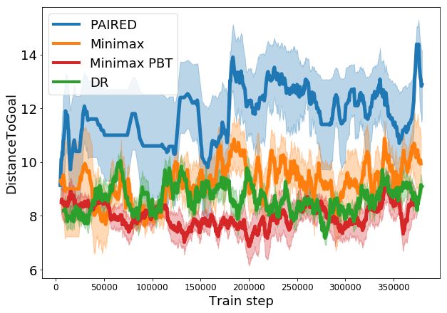
create challenging but feasible environments, in which the antagonist can outperform the protagonist.
Moreover, as the protagonist learns to solves the simple environments, the antagonist must generate
more complex environments to make the protagonist fail, increasing the complexity of the generated
tasks and leading to automatic curriculum generation.
We show that when both teams reach a Nash equilibrium, the generated environments have the highest
regret, in which the performance of the protagonist’s policy most differs from that of the optimal
policy. Thus, we call our approach Protagonist Antagonist Induced Regret Environment Design
(PAIRED). Our results demonstrate that compared to domain randomization, minimax adversarial
training, and population-based minimax training (as in Wang et al. [47]), PAIRED agents learn
more complex behaviors, and have higher zero-shot transfer performance in challenging, novel
environments.
In summary, our main contributions are: a) formalizing the problem of Unsupervised Environment
Design (UED) (Section 3), b) introducing the PAIRED Algorithm (Section 4), c) demonstrating
PAIRED leads to more complex behavior and more effective zero-shot transfer to new environments
than existing approaches to environment design (Section 5), and d) characterizing solutions to UED
and connecting the framework to classical decision theory (Section 3).

2   Related Work

When proposing an approach to UED we are essentially making a decision about which environments
to prioritize during training, based on an underspecified environment set provided by the designer.
Making decisions in situations of extreme uncertainty has been studied in decision theory under the
name “decisions under ignorance” [29] and is in fact deeply connected to our work, as we detail in
Section 3. Milnor [26] characterize several of these approaches; using Milnor’s terminology, we see
domain randomization [17] as “the principle of insufficient reason” proposed by Laplace, minimax
adversarial training [20] as the “maximin principle” proposed by Wald [46], and our approach,
PAIRED, as “minimax regret” proposed by Savage [35]. Savage’s approach was built into a theory of
making sequential decisions which minimize worst case regret [33, 21], which eventually developed
into modern literature on minimizing worst case regret in bandit settings [6].
Multi-agent training has been proposed as a way to automatically generate curricula in RL [22, 23, 14].
Competition can drive the emergence of complex skills, even some that the developer did not
anticipate [5, 13]. Asymmetric Self Play (ASP) [40] trains a demonstrator agent to complete the
simplest possible task that a learner cannot yet complete, ensuring that the task is, in principle,
solvable. In contrast, PAIRED is significantly more general because it generates complex new
environments, rather than trajectories within an existing, limited environment. Campero et al. [7]
study curriculum learning in a similar environment to the one under investigation in this paper. They
use a teacher to propose goal locations to which the agent must navigate, and the teacher’s reward
is computed based on whether the agent takes more or less steps than a threshold value. To create
a curriculum, the threshold is linearly increased over the course of training. POET [47, 48] uses
a population of minimax (rather than minimax regret) adversaries to generate the terrain for a 2D
walker. However, POET [47] requires generating many new environments, testing all agents within
each one, and discarding environments based on a manually chosen reward threshold, which wastes a
significant amount of computation. In contrast, our minimax regret approach automatically learns
to tune the difficulty of the environment by comparing the protagonist and antagonist’s scores. In
addition, these works do not investigate whether adversarial environment generation can provide
enhanced generalization when agents are transferred to new environments, as we do in this paper.
Environment design has also been investigated within the symbolic AI community. The problem of
modifying an environment to influence an agent’s decisions is analyzed in Zhang et al. [52], and was
later extended through the concept of Value-based Policy Teaching [51]. Keren et al. [18, 19] use a
heuristic best-first search to redesign an MDP to maximize expected value.
We evaluated PAIRED in terms of its ability to learn policies that transfer to unseen, hand-designed
test environments. One approach to produce policies which can transfer between environments is
unsupervised RL (e.g., [36, 38]). Gupta et al. [15] propose an unsupervised meta-RL technique
that computes minimax regret against a diverse task distribution learned with the DIAYN algorithm
[10]. However, this algorithm does not learn to modify the environment and does not adapt the
task distribution based on the learning progress of the agent. PAIRED provides a curriculum of

                                                  3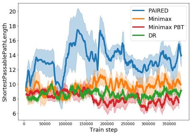
increasingly difficult environments and allows us to provide a theoretical characterization of when
minimax regret should be preferred over other approaches.
The robust control literature has made use of both minimax and regret objectives. Minimax training
has been used in the controls literature [39, 3, 53], the Robust MDP literature [4, 16, 28, 41], and
more recently, through the use of adversarial RL training [30, 45, 27]. Unlike our algorithm, minimax
adversaries have no incentive to guide the learning progress of the agent and can make environments
arbitrarily hard or unsolvable. Ghavamzadeh et al. [12] minimize the regret of a model-based policy
against a safe baseline to ensure safe policy improvement. Regan and Boutilier [31, 32] study Markov
Decision Processes (MDPs) in which the reward function is not fully specified, and use minimax
regret as an objective to guide the elicitation of user preferences. While these approaches use similar
theoretical techniques to ours, they use analytical solution methods that do not scale to the type of
deep learning approach used in this paper, do not attempt to learn to generate environments, and do
not consider automatic curriculum generation.
Domain randomization (DR) [17] is an alternative approach in which a designer specifies a set of
parameters to which the policy should be robust [34, 43, 42]. These parameters are then randomly
sampled for each episode, and a policy is trained that performs well on average across parameter
values. However, this does not guarantee good performance on a specific, challenging configuration
of parameters. While DR has had empirical success [1], it requires careful parameterization and
does not automatically tailor generated environments to the current proficiency of the learning agent.
Mehta et al. [25] propose to enhance DR by learning which parameter values lead to the biggest
decrease in performance compared to a reference environment.

3   Unsupervised Environment Design

The goal of this work is to construct a policy that performs well across a large set of environments.
We train policies by starting with an initially random policy, generating environments based on
that policy to best suit its continued learning, train that policy in the generated environments, and
repeat until the policy converges or we run out of resources. We then test the trained policies in
a set of challenging transfer tasks not provided during training. In this section, we will focus on
the environment generation step, which we call unsupervised environment design (UED). We will
formally define UED as the problem of using an underspecified environment to produce a distribution
over fully specified environments, which supports the continued learning of a particular policy. To do
this, we must formally define fully specified and underspecified environments, and describe how to
create a distribution of environments using UED. We will end this section by proposing minimax
regret as a novel approach to UED.
We will model our fully specified environments with a Partially Observable Markov Decision
Process (POMDP), which is a tuple hA, O, S , T , I , R, γi where A is a set of actions, O is a set of
observations, S is a set of states, T : S × A → ∆(S) is a transition function, I : S → O is an
observation (or inspection) function, R : S → R, and γ is a discount factor. We will define the utility
           PT
as U (π) = i=0 rt γ t , where T is a horizon.
To model an underspecified environment, we propose the Underspecified Partially Observable
Markov Decision Process (UPOMDP) as a tuple M = hA, O, Θ, S M , T M , I M , RM , γi. The only
difference between a POMDP and a UPOMDP is that a UPOMDP has a set Θ representing the
free parameters of the environment, which can be chosen to be distinct at each time step and are
incorporated into the transition function as T M : S × A × Θ → ∆(S). Thus a possible setting of
the environment is given by some trajectory of environment parameters θ.~ As an example UPOMDP,
                                           ~
consider a simulation of a robot in which θ are additional forces which can be applied at each time
step. A setting of the environment θ~ can be naturally combined with the underspecified environment
M to give a specific POMDP, which we will denote Mθ~ .
In UED, we want to generate a distribution of environments in which to continue training a policy.
We would like to curate this distribution of environments to best support the continued learning of a
particular agent policy. As such, we can propose a solution to UED by specifying some environment
policy, Λ : Π → ∆(ΘT ) where Π is the set of possible policies and ΘT is the set of possible
sequences of environment parameters. In Table 2, we see a few examples of possible choices for
environment policies, as well as how they correspond to previous literature. Each of these choices also

                                                  4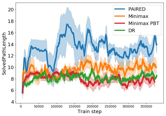
Table 1: Example Environment Policies
    UED Technique                         Environment Policy                           Decision Rule
                                             DR              T
    Domain Randomization [17, 34, 43]      Λ (π) = U(Θ )                               Insufficient Reason
                                                             ~
    Minimax Adversary [30, 45, 27]         ΛM (π) = argmin{U θ (π)}                    Maximin
                                                        ~
                                                        θ∈ΘT

  PAIRED (ours)                            ΛM R (π) = {θπ : vcππ , D̃π : otherwise} Minimax Regret
Table 2: The environment policies corresponding to the three techniques for UED which we study,
along with their corresponding decision rule. Where U(X) is a uniform distribution over X, D̃π is
a baseline distribution, θπ is the trajectory which maximizes regret of π, vπ is the value above the
baseline distribution that π achieves on that trajectory, and cπ is the negative of the worst-case regret
of π, normalized so that vcππ is between 0 and 1. This is described in full in the appendix.

have a corresponding decision rule used for making decisions under ignorance [29]. Each decision
rule can be understood as a method for choosing a policy given an underspecified environment. This
connection between UED and decisions under ignorance extends further than these few decision rules.
In the Appendix we will make this connection concrete and show that, under reasonable assumptions,
UED and decisions under ignorance are solving the same problem.
PAIRED can be seen as an approach for approximating the environment policy, ΛM R , which
corresponds to the decision rule minimax regret. One useful property of minimax regret, which
is not true of domain randomization or minimax adversarial training, is that whenever a task has
a sufficiently well-defined notion of success and failure it chooses policies which succeed. By
minimizing the worst case difference between what is achievable and what it achieves, whenever
there is a policy which ensures success, it will not fail where others could succeed.
Theorem 1. Suppose that all achievable rewards fall into one of two class of outcomes labeled
SUCCESS giving rewards in [Smin , Smax ] and FAILURE giving rewards in [Fmin , Fmax ], such
that Fmin ≤ Fmax < Smin ≤ Smax . In addition assume that the range of possible rewards in either
class is smaller than the difference between the classes so we have Smax − Smin < Smin − Fmax
and Fmax − Fmin < Smin − Fmax . Further suppose that there is a policy π which succeeds on any
θ~ whenever success is possible. Then minimax regret will choose a policy which has that property.

The proof of this property, and examples showing how minimax and domain randomization fail to
have this property, are in the Appendix. In the next section we will formally introduce PAIRED as a
method for approximating the minimax regret environment policy, ΛM R .

4     Protagonist Antagonist Induced Regret Environment Design (PAIRED)
Here, we describe how to approximate minimax regret, and introduce our proposed algorithm,
Protagonist Antagonist Induced Regret Environment Design (PAIRED). Regret is defined as the
difference between the payoff obtained for a decision, and the optimal payoff that could have been
obtained in the same setting with a different decision. In order to approximate regret, we use the
difference between the payoffs of two agents acting under the same environment conditions. Assume
                                                  ~ a fixed policy for the protagonist agent, π P , and
we are given a fixed environment with parameters θ,
                                          A
we then train a second antagonist agent, π , to optimality in this environment. Then, the difference
                                                  ~                               ~
between the reward obtained by the antagonist, U θ (π A ), and the protagonist, U θ (π P ), is the regret:
                                    ~                ~             ~
                            R EGRETθ π P , π A = U θ π A − U θ π P

                                                                                                      (1)
In PAIRED, we introduce an environment adversary that learns to control the parameters of the
environment, θ,~ to maximize the regret of the protagonist against the antagonist. For each training
batch, the adversary generates the parameters of the environment, θ~ ∼ Λ̃, which both agents will play.
The adversary and antagonist are trained to maximize the regret as computed in Eq. 1, while the
protagonist learns to minimize regret. This procedure is shown in Algorithm 1. The code for PAIRED
and our experiments is available in open source at https://github.com/google-research/

                                                    5
google-research/tree/master/social_rl/. We note that our approach is agnostic to the
choice of RL technique used to optimize regret.
To improve the learning signal for the adversary, once the adversary creates an environment, both
the protagonist and antagonist generate several trajectories within that same environment. This
allows for a more accurate approximation the minimax regret as the difference between the maximum
reward of the antagonist and the average reward of the protagonist over all trajectories: R EGRET ≈
          ~                 ~
maxτ A U θ (τ A ) − Eτ P [U θ (τ P )]. We have found this reduces noise in the reward and more accurately
rewards the adversary for building difficult but solvable environments.

Algorithm 1: PAIRED.
Randomly initialize Protagonist π P , Antagonist π A , and Adversary Λ̃;
while not converged do
   Use adversary to generate environment parameters: θ~ ∼ Λ̃. Use to create POMDP Mθ~ .
                                                            ~        PT
   Collect Protagonist trajectory τ P in Mθ~ . Compute: U θ (π P ) = i=0 rt γ t
                                                           ~        PT
   Collect Antagonist trajectory τ A in Mθ~ . Compute: U θ (π A ) = i=0 rt γ t
                        ~                    ~            ~
   Compute: R EGRETθ (π P , π A ) = U θ (π A ) − U θ (π P )
   Train Protagonist policy π P with RL update and reward R(τ P ) = −R EGRET
   Train Antagonist policy π A with RL update and reward R(τ A ) = R EGRET
   Train Adversary policy Λ̃ with RL update and reward R(τ Λ̃ ) = R EGRET
end

At each training step, the environment adversary can be seen as solving a UED problem for the current
protagonist, generating a curated set of environments in which it can learn. While the adversary
is motivated to generate tasks beyond the protagonist’s abilities, the regret can actually incentivize
creating the easiest task on which the protagonist fails but the antagonist succeeds. This is because if
the reward function contains any bonus for solving the task more efficiently (e.g. in fewer timesteps),
the antagonist will get more reward if the task is easier. Thus, the adversary gets the most regret for
proposing the easiest task which is outside the protagonist’s skill range. Thus, regret incentivizes the
adversary to propose tasks within the agent’s “zone of proximal development” [8]. As the protagonist
learns to solve the simple tasks, the adversary is forced to find harder tasks to achieve positive reward,
increasing the complexity of the generated tasks and leading to automatic curriculum generation.
Though multi-agent learning may not always converge [24], we can show that, if each team in this
game finds an optimal solution, the protagonist would be playing a minimax regret policy.
                            ~ be in Nash equilibrium and the pair (π A , θ)
Theorem 2. Let (π P , π A , θ)                                           ~ be jointly a best response
                                                          ~
to π P . Then π P ∈ argmin{ argmax {R EGRETθ (π P , π A )}}.
                    π P ∈ΠP          ~
                                π A ,θ∈ΠA ×ΘT

                        ~ be in Nash equilibria and the pair (π A , θ)
Proof. Let (π P , π A , θ)                                          ~ is jointly a best response to π P .
                           A ~                                                             ~
Then we can consider (π , θ) as one player with policy which we will write as π A+θ ∈ Π × ΘT .
           ~                                                                         ~ is jointly a best
Then π A+θ is in a zero sum game with π P , and the condition that the pair (π A , θ)
              P                              A+θ~                                              ~
response to π is equivalent to saying that π      is a best response to π . Thus π and π A+θ form a
                                                                          P         P

Nash equilibria of a zero sum game, and the minimax theorem applies. Since the reward in this game
is defined by R EGRET we have:
                                                                 ~
                            π P ∈ argmin{ argmax {R EGRETθ (π P , π A )}}
                                   π P ∈ΠP   π A+θ~ ∈Π×ΘT

                            ~
By the definition of π A+θ this proves the protagonist learns the minimax regret policy.

The proof gives us reason to believe that the iterative PAIRED training process in Algorithm 1 can
produce minimax regret policies. In Appendix D we show that if the agents are in Nash equilibrium,
without the coordination assumption, the protagonist will perform at least as well as the antagonist
in every parameterization, and Appendix E.1 provides empirical results for alternative methods for
approximating regret which break the coordination assumption. In the following sections, we will

                                                      6
show that empirically, policies trained with Algorithm 1 exhibit good performance and transfer, both
in generating emergent complexity and in training robust policies.

5     Experiments
The experiments in this section focus on assessing whether training with PAIRED can increase the
complexity of agents’ learned behavior, and whether PAIRED agents can achieve better or more
robust performance when transferred to novel environments. To study these questions, we first focus
on the navigation tasks shown in Figure 1. Section 5.2 presents results in continuous domains.

5.1     Partially Observable Navigation Tasks

Here we investigate navigation tasks (based on [9]), in which an agent must explore to find a
goal (green square in Figure 1) while navigating around obstacles. The environments are partially
observable; the agent’s field of view is shown as a blue shaded area in the figure. To deal with the
partial observability, we parameterize the protagonist and antagonist’s policies using recurrent neural
networks (RNNs). All agents are trained with PPO [37]. Further details about network architecture
and hyperparameters are given in Appendix F.
We train adversaries that learn to build these environments by choosing the location of the obstacles,
the goal, and the starting location of the agent. The adversary’s observations consist of a fully observed
view of the environment state, the current timestep t, and a random vector z ∼ N (0, I), z ∈ RD
sampled for each episode. At each timestep, the adversary outputs the location where the next
object will be placed; at timestep 0 it places the agent, 1 the goal, and every step afterwards an
obstacle. Videos of environments being constructed and transfer performance are available at
https://www.youtube.com/channel/UCI6dkF8eNrCz6XiBJlV9fmw/videos.

5.1.1    Comparison to Prior Methods
To compare to prior work that uses pure minimax training [30, 45, 27] (rather than minimax regret),
we use the same parameterization of the environment adversary and protagonist, but simply remove
the antagonist agent. The adversary’s reward is R(Λ) = −Eτ P [U (τ P )]. While a direct comparison
to POET [47] is challenging since many elements of the POET algorithm are specific to a 2D walker,
the main algorithmic distinction between POET and minimax environment design is maintaining
a population of environment adversaries and agents that are periodically swapped with each other.
Therefore, we also employ a Population Based Training (PBT) minimax technique in which the
agent and adversary are sampled from respective populations for each episode. This baseline is our
closest approximation of POET [47]. To apply domain randomization, we simply sample the (x, y)
positions of the agent, goal, and blocks uniformly at random. We sweep shared hyperparameters for
all methods equally. Parameters for the emergent complexity task are selected to maximize the solved
path length, and parameters for the transfer task are selected using a set of validation environments.
Details are given in the appendix.

5.1.2    Emergent Complexity
Prior work [47, 48] focused on demonstrating emergent complexity as the primary goal, arguing that
automatically learning complex behaviors is key to improving the sophistication of AI agents. Here,
we track the complexity of the generated environments and learned behaviors throughout training.
Figure 2 shows the number of blocks (a), distance to the goal (b), and the length of the shortest path
to the goal (c) in the generated environments. The solved path length (d) tracks the shortest path
length of a maze that the agent has completed successfully, and can be considered a measure of the
complexity of the agent’s learned behavior.
Domain randomization (DR) simply maintains environment parameters within a fixed range, and
cannot continue to propose increasingly difficult tasks. Techniques based on minimax training are
purely motivated to decrease the protagonist’s score, and as such do not enable the agent to continue
learning; both minimax and PBT obtain similar performance to DR. In contrast, PAIRED creates a
curriculum of environments that begin with shorter paths and fewer blocks, but gradually increase in
complexity based on both agents’ current level of performance. As shown in Figure 2 (d), this allows
PAIRED protagonists to learn to solve more complex environments than the other two techniques.

                                                    7
(a) Number of blocks         (b) Distance to goal       (c) Passable path length    (d) Solved path length
Figure 2: Statistics of generated environments in terms of the number of blocks (a), distance from the
start position to the goal (b), and the shortest path length between the start and the goal, which is zero
if there is no possible path (c). The final plot shows agent learning in terms of the shortest path length
of a maze successfully solved by the agents. Each plot is measured over five random seeds; error bars
are a 95% CI. Domain randomization (DR) cannot tailor environment design to the agent’s progress,
so metrics remain fixed or vary randomly. Minimax training (even with populations of adversaries
and agents) has no incentive to improve agent performance, so the length of mazes that agents are
able to solve remains similar to DR (d). In contrast, PAIRED is the only method that continues to
increase the passable path length to create more challenging mazes (c), producing agents that solve
more complex mazes than the other techniques (d).

        (a) Empty   (b) 50 Blocks      (c) 4 Rooms        (d) 16 Rooms      (e) Labyrinth      (f) Maze
Figure 3: Percent successful trials in environments used to test zero-shot transfer, out of 10 trials
each for 5 random seeds. The first two (a, b) simply test out-of-distribution generalization to a setting
of the number of blocks parameter. Four Rooms (c) tests within-distribution generalization to a
specific configuration that is unlikely to be generated through random sampling. The 16 Rooms (d),
Labyrinth environment (e) and Maze (f) environments were designed by a human to be challenging
navigation tasks. The bar charts show the zero-shot transfer performance of models trained with
domain randomization (DR), minimax, or PAIRED in each of the environments. Error bars show a
95% confidence interval. As task difficulty increases, only PAIRED retains its ability to generalize to
the transfer tasks.

5.1.3     Zero-Shot Transfer
In order for RL algorithms to be useful in the real world, they will need to generalize to novel
environment conditions that their developer was not able to foresee. Here, we test the zero-shot
transfer performance on a series of novel navigation tasks shown in Figure 3. The first two transfer
tasks simply use a parameter setting for the number of blocks that is out of the distribution (OOD)
of the training environments experienced by the agents (analogous to the evaluation of [30]). We
expect these transfer scenarios to be easy for all methods. We also include a more structured but still
very simple Four Rooms environment, where the number of blocks is within distribution, but in an
unlikely (though simple) configuration. As seen in the figure, this can usually be completed with
nearly straight-line paths to the goal. To evaluate difficult transfer settings, we include the 16 rooms,
Labyrinth, and Maze environments, which require traversing a much longer and more challenging
path to the goal. This presents a much more challenging transfer scenario, since the agent must learn
meaningful navigation skills to succeed in these tasks.
Figure 3 shows zero-shot transfer performance. As expected, all methods transfer well to the first
two environments, although the minimax adversary is significantly worse in 50 Blocks. Varying the
number of blocks may be a relatively easy transfer task, since partial observability has been shown to

                                                      8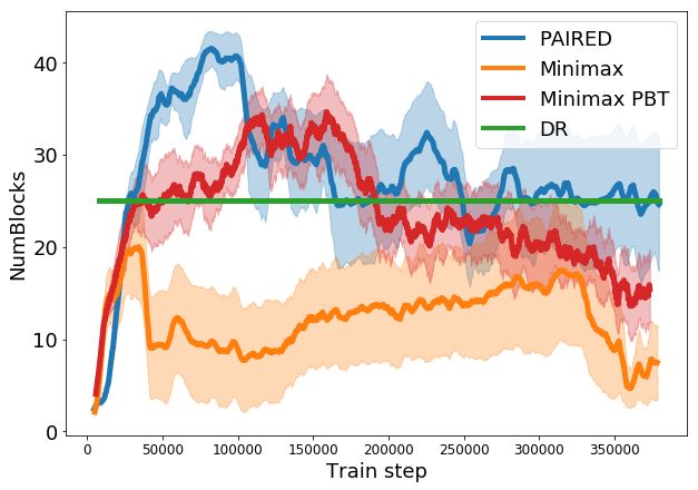
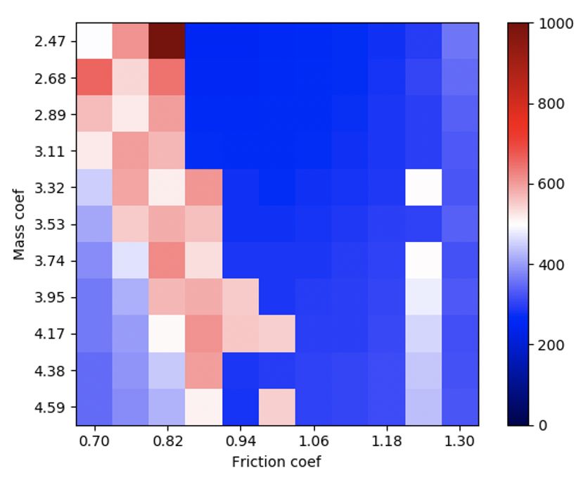
(a) Reward                   (b) Minimax Adversarial              (c) PAIRED
Figure 4: Training curves for PAIRED and minimax adversaries on the MuJoCo hopper, where
adversary strength is scaled up over the first 300 iterations (a). While both adversaries reduce the
agent’s reward by making the task more difficult, the minimax adversary is incentivized to drive
the agent’s reward as low as possible. In contrast, the PAIRED adversary must maintain feasible
parameters. When varying force and mass are applied at test time, the minimax policy performs
poorly in cumulative reward (b), while PAIRED is more robust (c).

improve generalization performance in grid-worlds [49]. As the environments increase in difficulty,
so does the performance gap between PAIRED and the prior methods. In 16 Rooms, Labyrinth,
and Maze, PAIRED shows a large advantage over the other two methods. In the Labyrinth (Maze)
environment, PAIRED agents are able to solve the task in 40% (18%) of trials. In contrast, minimax
agents solve 10% (0.0%) of trials, and DR agents solve 0.0%. The performance of PAIRED on these
tasks can be explained by the complexity of the generated environments; as shown in Figure 1c, the
field of view of the agent (shaded blue) looks similar to what it might encounter in a maze, although
the idea of a maze was never explicitly specified to the agent, and this configuration blocks is very
unlikely to be generated randomly. These results suggest that PAIRED training may be better able to
prepare agents for challenging, unknown test settings.

5.2   Continuous Control Tasks

To compare more closely with prior work on minimax adversarial RL [30, 45], we construct an
additional experiment in a modified version of the MuJoCo hopper domain [44]. Here, the adversary
                                                                           ~ We benchmark PAIRED
outputs additional torques to be applied to each joint at each time step, θ.
against unconstrained minimax training. To make minimax training feasible, the torque the adversary
can apply is limited to be a proportion of the agent’s strength, and is scaled from 0.1 to 1.0 over the
course of 300 iterations. After this point, we continue training with no additional mechanisms for
constraining the adversary. We pre-train the agents for 100 iterations, then test transfer performance
to a set of mass and friction coefficients. All agents are trained with PPO [37] and feed-forward
policies.
Figure 4a shows the rewards throughout training. We observe that after the constraints on the
adversaries are removed after 300 iterations, the full-strength minimax adversary has the ability to
make the task unsolvable, so the agent’s reward is driven to zero for the rest of training. In contrast,
PAIRED is able to automatically adjust the difficulty of the adversary to ensure the task remains
solvable. As expected, Figure 4 shows that when constraints on the adversary are not carefully tuned,
policies trained with minimax fail to learn and generalize to unseen environment parameters. In
contrast, PAIRED agents are more robust to unseen environment parameters, even without careful
tuning of the forces that the adversary is able to apply.

6     Conclusions
We develop the framework of Unsupervised Environment Design (UED), and show its relevance to a
range of RL tasks, from learning increasingly complex behavior or more robust policies, to improving
generalization to novel environments. In environments like games, for which the designer has an
accurate model of the test environment, or can easily enumerate all of the important cases, using
UED may be unnecessary. However, UED could provide an approach to building AI systems in many
of the ambitious uses of AI in real-world settings which are difficult to accurately model.

                                                   9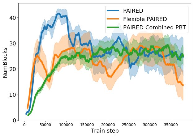
We have shown that tools from the decision theory literature can be used to characterize existing
approaches to environment design, and motivate a novel approach based on minimax regret. Our
algorithm, which we call Protagonist Antagonist Induced Regret Environment Design (PAIRED),
avoids common failure modes of existing UED approaches, and is able to generate a curriculum of
increasingly complex environments. Our results demonstrate that PAIRED agents learn more complex
behaviors, and achieve higher zero-shot transfer performance in challenging, novel environments.

Broader Impact

Unsupervised environment design is a technique with a wide range of applications, including un-
supervised RL, transfer learning, and Robust RL. Each of these applications has the chance of
dramatically improving the viability of real-world AI systems. Real-world AI systems could have
a variety of positive impacts, reducing the possibility for costly human error, increasing efficiency,
and doing tasks that are dangerous or difficult for humans. However, there are a number of possible
negative impacts: increasing unemployment by automating jobs [11] and improving the capabilities
of automated weapons. These positives and negatives are potentially exacerbated by the emergent
complexity we described in Section 5.1.2, which could lead to improved efficiency and generality
allowing the robotics systems to be applied more broadly.
However, if we are to receive any of the benefits of AI powered systems being deployed into real
world settings, it is critical that we know how to make these systems robust and that they know how
to make good decisions in uncertain environments. In Section 3 we discussed the deep connections
between UED and decisions under ignorance, which shows that reasonable techniques for making
decisions in uncertain settings correspond to techniques for UED, showing that the study of UED
techniques can be thought of as another angle of attack at the problem of understanding how to make
robust systems. Moreover, we showed in Section 5.2 that these connections are not just theoretical,
but can lead to more effective ways of building robust systems. Continued work in this area can help
ensure that the predominant impact of our AI systems is the impact we intended.
Moreover, many of the risks of AI systems come from the system acting unexpectedly in a situation the
designer had not considered. Approaches for Unsupervised Environment Design could work towards
a solution to this problem, by automatically generating interesting and challenging environments,
hopefully detecting troublesome cases before they appear in deployment settings.

Acknowledgments and Disclosure of Funding

We would like to thank Michael Chang, Marvin Zhang, Dale Schuurmans, Aleksandra Faust, Chase
Kew, Jie Tan, Dennis Lee, Kelvin Xu, Abhishek Gupta, Adam Gleave, Rohin Shah, Daniel Filan,
Lawrence Chan, Sam Toyer, Tyler Westenbroek, Igor Mordatch, Shane Gu, DJ Strouse, and Max
Kleiman-Weiner for discussions that contributed to this work. We are grateful for funding of this
work as a gift from the Berkeley Existential Risk Intuitive. We are also grateful to Google Research
for funding computation expenses associated with this work.

References
 [1] OpenAI: Marcin Andrychowicz, Bowen Baker, Maciek Chociej, Rafal Jozefowicz, Bob Mc-
     Grew, Jakub Pachocki, Arthur Petron, Matthias Plappert, Glenn Powell, Alex Ray, et al. Learning
     dexterous in-hand manipulation. The International Journal of Robotics Research, 39(1):3–20,
     2020.

 [2] Rika Antonova, Silvia Cruciani, Christian Smith, and Danica Kragic. Reinforcement learning
     for pivoting task. arXiv preprint arXiv:1703.00472, 2017.

 [3] Karl Johan Åström. Theory and applications of adaptive control—a survey. Automatica, 19(5):
     471–486, 1983.

 [4] J Andrew Bagnell, Andrew Y Ng, and Jeff G Schneider. Solving uncertain markov decision
     processes. 2001.

                                                 10
[5] Bowen Baker, Ingmar Kanitscheider, Todor Markov, Yi Wu, Glenn Powell, Bob McGrew,
and Igor Mordatch. Emergent tool use from multi-agent autocurricula. arXiv preprint
arXiv:1909.07528, 2019.
[6] Sébastien Bubeck and Nicolo Cesa-Bianchi. Regret analysis of stochastic and nonstochastic
multi-armed bandit problems. arXiv preprint arXiv:1204.5721, 2012.
[7] Andres Campero, Roberta Raileanu, Heinrich Küttler, Joshua B Tenenbaum, Tim Rocktäschel,
and Edward Grefenstette. Learning with amigo: Adversarially motivated intrinsic goals. arXiv
preprint arXiv:2006.12122, 2020.
[8] Seth Chaiklin et al. The zone of proximal development in vygotsky’s analysis of learning and
instruction. Vygotsky’s educational theory in cultural context, 1(2):39–64, 2003.
[9] Maxime Chevalier-Boisvert, Lucas Willems, and Suman Pal. Minimalistic gridworld environ-
ment for openai gym. https://github.com/maximecb/gym-minigrid, 2018.
[10] Benjamin Eysenbach, Abhishek Gupta, Julian Ibarz, and Sergey Levine. Diversity is all you
need: Learning skills without a reward function. arXiv preprint arXiv:1802.06070, 2018.
[11] Carl Benedikt Frey and Michael A Osborne. The future of employment: How susceptible are
jobs to computerisation? Technological forecasting and social change, 114:254–280, 2017.
[12] Mohammad Ghavamzadeh, Marek Petrik, and Yinlam Chow. Safe policy improvement by
minimizing robust baseline regret. In Advances in Neural Information Processing Systems,
pages 2298–2306, 2016.
[13] Adam Gleave, Michael Dennis, Cody Wild, Neel Kant, Sergey Levine, and Stuart Russell.
Adversarial policies: Attacking deep reinforcement learning. In International Conference on
Learning Representations, 2020.
[14] Alex Graves, Marc G Bellemare, Jacob Menick, Remi Munos, and Koray Kavukcuoglu. Auto-
mated curriculum learning for neural networks. arXiv preprint arXiv:1704.03003, 2017.
[15] Abhishek Gupta, Benjamin Eysenbach, Chelsea Finn, and Sergey Levine. Unsupervised
meta-learning for reinforcement learning. arXiv preprint arXiv:1806.04640, 2018.
[16] Garud N Iyengar. Robust dynamic programming. Mathematics of Operations Research, 30(2):
257–280, 2005.
[17] Nick Jakobi. Evolutionary robotics and the radical envelope-of-noise hypothesis. Adaptive
behavior, 6(2):325–368, 1997.
[18] Sarah Keren, Luis Pineda, Avigdor Gal, Erez Karpas, and Shlomo Zilberstein. Equi-reward
utility maximizing design in stochastic environments. HSDIP 2017, page 19, 2017.
[19] Sarah Keren, Luis Pineda, Avigdor Gal, Erez Karpas, and Shlomo Zilberstein. Efficient heuristic
search for optimal environment redesign. In Proceedings of the International Conference on
Automated Planning and Scheduling, volume 29, pages 246–254, 2019.
[20] Rawal Khirodkar, Donghyun Yoo, and Kris M Kitani. Vadra: Visual adversarial domain
randomization and augmentation. arXiv preprint arXiv:1812.00491, 2018.
[21] Tze Leung Lai and Herbert Robbins. Asymptotically efficient adaptive allocation rules. Ad-
vances in applied mathematics, 6(1):4–22, 1985.
[22] Joel Z Leibo, Edward Hughes, Marc Lanctot, and Thore Graepel. Autocurricula and the
emergence of innovation from social interaction: A manifesto for multi-agent intelligence
research. arXiv preprint arXiv:1903.00742, 2019.
[23] Tambet Matiisen, Avital Oliver, Taco Cohen, and John Schulman. Teacher-student curriculum
learning. IEEE transactions on neural networks and learning systems, 2019.
[24] Eric Mazumdar, Lillian J Ratliff, and S Shankar Sastry. On gradient-based learning in continuous
games. SIAM Journal on Mathematics of Data Science, 2(1):103–131, 2020.
11[25] Bhairav Mehta, Manfred Diaz, Florian Golemo, Christopher J Pal, and Liam Paull. Active
domain randomization. In Conference on Robot Learning, pages 1162–1176. PMLR, 2020.
[26] John Milnor. Games against nature. Decision Processes, pages 49–59, 1954.
[27] Jun Morimoto and Kenji Doya. Robust reinforcement learning. In Advances in neural informa-
tion processing systems, pages 1061–1067, 2001.
[28] Arnab Nilim and Laurent El Ghaoui. Robust control of markov decision processes with uncertain
transition matrices. Operations Research, 53(5):780–798, 2005.
[29] Martin Peterson. An introduction to decision theory. Cambridge University Press, 2017.
[30] Lerrel Pinto, James Davidson, and Abhinav Gupta. Supervision via competition: Robot adver-
saries for learning tasks. In 2017 IEEE International Conference on Robotics and Automation
(ICRA), pages 1601–1608. IEEE, 2017.
[31] Kevin Regan and Craig Boutilier. Robust online optimization of reward-uncertain mdps. In
Twenty-Second International Joint Conference on Artificial Intelligence. Citeseer, 2011.
[32] Kevin Regan and Craig Boutilier. Regret-based reward elicitation for markov decision processes.
arXiv preprint arXiv:1205.2619, 2012.
[33] Herbert Robbins. Some aspects of the sequential design of experiments. Bulletin of the American
Mathematical Society, 58(5):527–535, 1952.
[34] Fereshteh Sadeghi and Sergey Levine. Cad2rl: Real single-image flight without a single real
image. arXiv preprint arXiv:1611.04201, 2016.
[35] Leonard J Savage. The theory of statistical decision. Journal of the American Statistical
association, 46(253):55–67, 1951.
[36] Jürgen Schmidhuber. Formal theory of creativity, fun, and intrinsic motivation (1990–2010).
IEEE Transactions on Autonomous Mental Development, 2(3):230–247, 2010.
[37] John Schulman, Filip Wolski, Prafulla Dhariwal, Alec Radford, and Oleg Klimov. Proximal
policy optimization algorithms. arXiv preprint arXiv:1707.06347, 2017.
[38] Pierre Sermanet, Corey Lynch, Yevgen Chebotar, Jasmine Hsu, Eric Jang, Stefan Schaal, Sergey
Levine, and Google Brain. Time-contrastive networks: Self-supervised learning from video. In
2018 IEEE International Conference on Robotics and Automation (ICRA), pages 1134–1141.
IEEE, 2018.
[39] Jean-Jacques E Slotine and Weiping Li. On the adaptive control of robot manipulators. The
international journal of robotics research, 6(3):49–59, 1987.
[40] Sainbayar Sukhbaatar, Zeming Lin, Ilya Kostrikov, Gabriel Synnaeve, Arthur Szlam, and Rob
Fergus. Intrinsic motivation and automatic curricula via asymmetric self-play. arXiv preprint
arXiv:1703.05407, 2017.
[41] Aviv Tamar, Shie Mannor, and Huan Xu. Scaling up robust mdps using function approximation.
In International Conference on Machine Learning, pages 181–189, 2014.
[42] Jie Tan, Tingnan Zhang, Erwin Coumans, Atil Iscen, Yunfei Bai, Danijar Hafner, Steven Bohez,
and Vincent Vanhoucke. Sim-to-real: Learning agile locomotion for quadruped robots. arXiv
preprint arXiv:1804.10332, 2018.
[43] Josh Tobin, Rachel Fong, Alex Ray, Jonas Schneider, Wojciech Zaremba, and Pieter Abbeel.
Domain randomization for transferring deep neural networks from simulation to the real world.
In 2017 IEEE/RSJ international conference on intelligent robots and systems (IROS), pages
23–30. IEEE, 2017.
[44] Emanuel Todorov, Tom Erez, and Yuval Tassa. Mujoco: A physics engine for model-based
control. In 2012 IEEE/RSJ International Conference on Intelligent Robots and Systems, pages
5026–5033. IEEE, 2012.
12[45] Eugene Vinitsky, Kanaad Parvate, Yuqing Du, Pieter Abbeel, and Alexandre Bayen. D-malt:
Diverse multi-adversarial learning for transfer 003. In Submission to ICML 2020).
[46] Abraham Wald. Statistical decision functions. 1950.
[47] Rui Wang, Joel Lehman, Jeff Clune, and Kenneth O Stanley. Paired open-ended trailblazer
(poet): Endlessly generating increasingly complex and diverse learning environments and their
solutions. arXiv preprint arXiv:1901.01753, 2019.
[48] Rui Wang, Joel Lehman, Aditya Rawal, Jiale Zhi, Yulun Li, Jeff Clune, and Kenneth O Stanley.
Enhanced poet: Open-ended reinforcement learning through unbounded invention of learning
challenges and their solutions. arXiv preprint arXiv:2003.08536, 2020.
[49] Chang Ye, Ahmed Khalifa, Philip Bontrager, and Julian Togelius. Rotation, translation, and
cropping for zero-shot generalization. arXiv preprint arXiv:2001.09908, 2020.
[50] Wenhao Yu, Jie Tan, C Karen Liu, and Greg Turk. Preparing for the unknown: Learning a
universal policy with online system identification. arXiv preprint arXiv:1702.02453, 2017.
[51] Haoqi Zhang and David C Parkes. Value-based policy teaching with active indirect elicitation.
In AAAI, volume 8, pages 208–214, 2008.
[52] Haoqi Zhang, Yiling Chen, and David C Parkes. A general approach to environment design
with one agent. 2009.
[53] Kemin Zhou, John Comstock Doyle, Keith Glover, et al. Robust and optimal control, volume 40.
Prentice hall New Jersey, 1996.
A Generality of UED
In Section 3 we defined UPODMPS and UED and showed a selection of natural approaches to
UED and corrisponding decision rules. However, the connection between UED and decisions under
ignorance is much broader than these few decision rules. In fact, they can be seen as nearly identical
problems.
To see the connection to decisions under ignorance, it is important to notice that any decision rule
can be thought of as an ordering over policies, ranking the policies that it chooses higher than other
policies. We will want to define a condition on this ordering, to do this we will first define what it
means for one policy to totally dominate another.
Definition 3. A policy, πA , is totally dominated by some policy, πB if for every pair of parameteriza-
M M
tions θ~A , θ~B U θ~A (πA ) < U θ~B (πB ).
Thus if πA totally dominates πB , it is reasonable to assume that πA is better, since the best outcome
we could hope for from policy πB is still worse than the worst outcome we fear from policy πA .
Thus we would hope that our decision rule would not prefer πB to πA . If a decision rule respects this
property we will say that it respects total domination or formally:
Definition 4. We will say that an ordering ≺ respects total domination iff πA ≺ πB whenever πB
totally dominates πA .
This is a very weak condition, but it is already enough to allow us to provide a characterization of all
such orderings over policies in terms of policy-conditioned distributions over parameters θ, ~ which
we will notate Λ as in Section 3. Specifically, any ordering which respects total domination can be
written as maximizing the expected value with respect to a policy-conditioned value function, thus
every reasonable way of ranking policies can be described in the UED framework. For example,
this implies that there is an environment policy which represents the strategy of minimax regret. We
explicitly construct one such environment policy in Appendix B.
To make this formal, the policy-conditioned value function, V MΛ (π), is defined to be the expected
value a policy will receive in the policy-conditioned distribution of environments MΛ(π) , or formally:
~
V MΛ (π) = E [U θ (π)] (2)
~
θ∼Λ(π)
13.
The policy-conditioned value function is like the normal value function, but computed over the
distribution of environments defined by the UPOMDP and environment policy. This of course implies
an ordering over policies, defined in the natural way.
Definition 5. We will say that Λ prefers πB to πA notated πA ≺Λ πB if V MΛ (πA ) < V MΛ (πB )
Finally, this allows us to state the main theorem of this Section.
Theorem 6. Given an order over deterministic policies in a finite UPOMDP, ≺, there exits an
environment policy Λ : Π → ∆(ΘT ) such that ≺ is equivalent to ≺Λ iff it respects total domination
and it ranks policies with an equal and a deterministic outcome as equal.
Proof. Suppose you have some order of policies in a finite UPOMDP, ≺, which respects total
domination and ranks policies equal if they have an equal and deterministic outcome. Our goal is to
construct a function Λ such that πA ≺Λ πB iff πA ≺ πB .
When constructing Λ notice that we can chose Λ(π) independently for each policy π and
that we can choose the resulting value for V MΛ (π) to lie anywhere within the range
~ ~
[ min {U θ (π)}, max {U θ (π)}]. Since the number of deterministic policies in a finite POMDP
~
θ∈ΘT ~
θ∈ΘT
is finite, we can build Λ inductively by taking the lowest ranked policy π in terms of ≺ for which Λ
has not yet been defined and choosing the value for V MΛ (π) appropriately.
For the lowest ranked policy πB for which Λ(πB ) has not yet been defined we set Λ(πB ) such that
V MΛ (πB ) greater than Λ(πA ) for all πA ≺ πB and is lower than the minimum possible value of
any πC such that πB ≺ πC , if such a setting is possible. That is, we choose Λ(πB ) to satisfy for all
πA ≺ πB ≺ πC :
~
Λ(πA ) < V MΛ (πB ) < max {U θ (πC )} (3)
~
θ∈ΘT
Intuitively this ensures that V MΛ (πB ) is high enough to be above all πA lower than πB and low
enough such that all future πC can still be assigned an appropriate value.
Finally, we will show that it is possible to set Λ(πB ) to satisfy these conditions in Equation 3. By our
~ ~
inductive hypothesis, we know that Λ(πA ) < max {U θ (πB )} and Λ(πA ) < max {U θ (πC )}. Since
~
θ∈ΘT ~
θ∈ΘT
~
θ ~
θ
≺ respects total domination, we know that min {U (πB )} ≤ max {U (πC )} for all πB ≤ πC .
~
θ∈ΘT ~
θ∈ΘT
Since there are a finite number of πC we can set V MΛ (πB ) to be the average of the smallest value
~
for max {U θ (πC )} and the largest value for Λ(πA ) for any πC and πA satisfying πA ≺ πB ≺ πC .
~
θ∈ΘT
The other direction, can be checked directly. If πA is totally dominated by πB , then:
~ ~
V MΛ (πA ) = E [U θ (πA )] < E [U θ (πB )] = V MΛ (πB )
~
θ∼Λ(πA)
~
θ∼Λ(πB)
Thus if ≺ can be represented with an appropriate choice of Λ then it respects total domination and it
ranks policies with an equal and a deterministic outcome equal.
Thus, the set of decision rules which respect total domination are exactly those which can be written
by some concrete environment policy, and thus any approach to making decisions under uncertainty
which has this property can be thought of as a problem of unsupervised environment design and
vice-versa. To the best of our knowledge there is no seriously considered approach to making
decisions under uncertainty which does not satisfy this property.
B Defining an Environment Policy Corresponding to Minimax Regret
In this section we will be deriving a function Λ(π) which corresponds to regret minimization. We
will be assuming a finite MDP with a bounded reward function. Explicitly, we will be deriving a Λ
14such that minimax regret is the decision rule which maximizes the corresponding policy-conditioned
value function defined in Appendix A:
~
V MΛ (π) = E [U θ (π)]
~
θ∼Λ(π)
In this context, we will define regret to be:
~ = max {U Mθ~ (π B ) − U Mθ~ (π)}
R EGRET(π, θ)
π B ∈Π
Thus the set of M INIMAX R EGRET strategies can be defined naturally as the ones which achive the
minimum worst case regret:
~
M INIMAX R EGRET = argmin{ max {R EGRET(π, θ)}}
π∈Π ~
θ∈ΘT
We want to find a function Λ for which the set of optimal policies which maximize value with respect
to Λ is the same as the set of M INIMAX R EGRET strategies. That is, we want to find Λ such that:
M INIMAX R EGRET = argmax{V MΛ (π)}
π∈Π
To do this it is useful to first introduce the concept of weak total domination, which is the natural
weakening of the concept of total domination introduced in Appendix A. A policy is said to be weakly
totally dominated by a policy πB if the maximum outcome that can be achieved by πA is equal to the
minimum outcome that can be achieved by πB , or formally:
Definition 7. A policy, πA , is weakly totally dominated by some policy, πB if for every pair of
M M
parameterizations θ~A , θ~B U θ~A (πA ) ≤ U θ~B (πB ).
The concept of weak total domination is only needed here to clarify what happens in the special case
that there are policies that are weakly totally dominated but not totally dominated. These policies
may or may not be minimax regret optimal policies, and thus have to be treated with more care. To
get a general sense for how the proof works you may assume that there are no policies which are
weakly totally dominated but not totally dominated and skip the sections of the proof marked as a
special case: the second paragraph of the proof for Lemma 8 and the second paragraph of the proof
for Theorem 9.
We can use this concept to help define a normalization function D : Π → ∆(ΘT ) which has the
property that if there are two policies πA , πB such that neither is totally dominated by the other,
then they evaluate the same value on the distribution of environments. We will use D as a basis for
creating Λ by shifting probability mass towards or away from this distribution in the right proportion.
In general there are many such normalization functions, but we will simply show that one of these
exists.
Lemma 8. There exists a function D : Π → ∆(ΘT ) such that Λ(π) has support at least s > 0 on
the highest-valued regret-maximizing parameterization θπ for all π, that for all πA , πB such that
neither is weakly totally dominated by any other policy, V MD (πA ) = V MD (πB ) and V MD (πA ) >
V MD (πB ) when πB is totally dominated and πA is not. If the policy π is weakly dominated but
not totally dominated we choose D to put full support on the highest-valued regret-maximizing
parameterization, D(π) = θπ .
Proof. We will first define D for the set of policies which are not totally dominated, which we will
call X. Note that by the definition of not being totally dominated, there is a constant C which is
between the worst-case and best-case values of all of the policies in X.
Special Case: If there is only one choice for C and if that does have support over θπ for each π
which is not totally dominated, then we know that there is a weakly totally dominated policy which is
not totally dominated. In this case we choose a C which is between the best-case and the worst-case
for the not weakly totally dominated policies. Thus for each π which is not weakly dominated we can
15You can also read