ERA5-Land: a state-of-the-art global reanalysis dataset for land applications
←
→
Page content transcription
If your browser does not render page correctly, please read the page content below
Earth Syst. Sci. Data, 13, 4349–4383, 2021
https://doi.org/10.5194/essd-13-4349-2021
© Author(s) 2021. This work is distributed under
the Creative Commons Attribution 4.0 License.
ERA5-Land: a state-of-the-art global
reanalysis dataset for land applications
Joaquín Muñoz-Sabater1 , Emanuel Dutra2,3 , Anna Agustí-Panareda1 , Clément Albergel4,5 ,
Gabriele Arduini1 , Gianpaolo Balsamo1 , Souhail Boussetta1 , Margarita Choulga1 , Shaun Harrigan1 ,
Hans Hersbach1 , Brecht Martens6 , Diego G. Miralles6 , María Piles7 , Nemesio J. Rodríguez-Fernández8 ,
Ervin Zsoter1 , Carlo Buontempo1 , and Jean-Noël Thépaut1
1 European Centre for Medium-range Weather Forecasts, Reading, UK
2 Instituto Português do Mar e da Atmosfera, Lisbon, Portugal
3 Instituto Dom Luiz, IDL, Faculty of Sciences, University of Lisbon, Lisbon, Portugal
4 CNRM, Université de Toulouse, Météo-France, CNRS, Toulouse, France
5 European Space Agency Climate Office, ECSAT, Didcot, UK
6 Hydro-Climate Extremes Lab (H-CEL), Ghent University, Ghent, Belgium
7 Image Processing Laboratory (IPL), Universitat de València, València, Spain
8 Centre d’Etudes Spatiales de la Biosphère (CESBIO),
Université Toulouse 3, CNES, CNRS, INRAE, IRDe, Toulouse, France
Correspondence: Joaquín Muñoz-Sabater (joaquin.munoz@ecmwf.int)
Received: 9 March 2021 – Discussion started: 15 March 2021
Revised: 17 June 2021 – Accepted: 6 July 2021 – Published: 7 September 2021
Abstract. Framed within the Copernicus Climate Change Service (C3S) of the European Commission, the Eu-
ropean Centre for Medium-Range Weather Forecasts (ECMWF) is producing an enhanced global dataset for the
land component of the fifth generation of European ReAnalysis (ERA5), hereafter referred to as ERA5-Land.
Once completed, the period covered will span from 1950 to the present, with continuous updates to support land
monitoring applications. ERA5-Land describes the evolution of the water and energy cycles over land in a con-
sistent manner over the production period, which, among others, could be used to analyse trends and anomalies.
This is achieved through global high-resolution numerical integrations of the ECMWF land surface model driven
by the downscaled meteorological forcing from the ERA5 climate reanalysis, including an elevation correction
for the thermodynamic near-surface state. ERA5-Land shares with ERA5 most of the parameterizations that
guarantees the use of the state-of-the-art land surface modelling applied to numerical weather prediction (NWP)
models. A main advantage of ERA5-Land compared to ERA5 and the older ERA-Interim is the horizontal res-
olution, which is enhanced globally to 9 km compared to 31 km (ERA5) or 80 km (ERA-Interim), whereas the
temporal resolution is hourly as in ERA5. Evaluation against independent in situ observations and global model
or satellite-based reference datasets shows the added value of ERA5-Land in the description of the hydrological
cycle, in particular with enhanced soil moisture and lake description, and an overall better agreement of river
discharge estimations with available observations. However, ERA5-Land snow depth fields present a mixed per-
formance when compared to those of ERA5, depending on geographical location and altitude. The description of
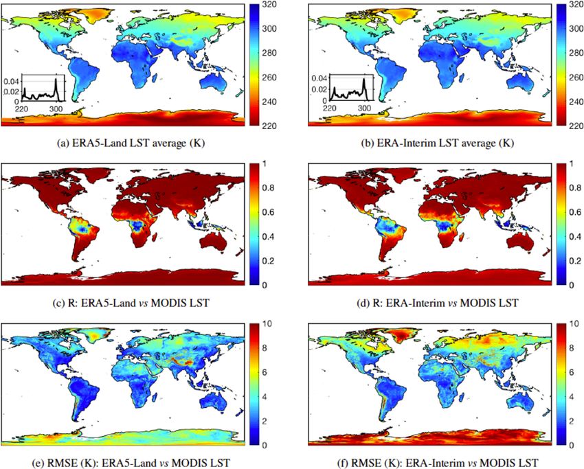
the energy cycle shows comparable results with ERA5. Nevertheless, ERA5-Land reduces the global averaged
root mean square error of the skin temperature, taking as reference MODIS data, mainly due to the contribution
of coastal points where spatial resolution is important. Since January 2020, the ERA5-Land period available has
extended from January 1981 to the near present, with a 2- to 3-month delay with respect to real time. The seg-
ment prior to 1981 is in production, aiming for a release of the whole dataset in summer/autumn 2021. The high
spatial and temporal resolution of ERA5-Land, its extended period, and the consistency of the fields produced
makes it a valuable dataset to support hydrological studies, to initialize NWP and climate models, and to support
diverse applications dealing with water resource, land, and environmental management.
Published by Copernicus Publications.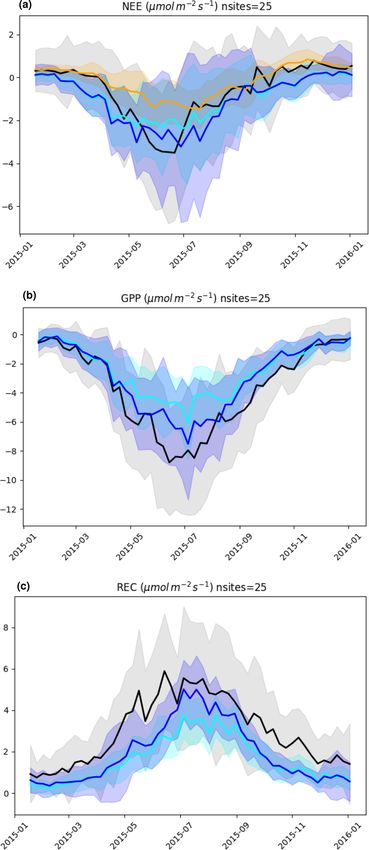
4350                                                                                      J. Muñoz-Sabater et al.: ERA5-Land

         The full ERA5-Land hourly (Muñoz-Sabater, 2019a) and monthly (Muñoz-Sabater, 2019b) averaged datasets
       presented in this paper are available through the C3S Climate Data Store at https://doi.org/10.24381/cds.
       e2161bac and https://doi.org/10.24381/cds.68d2bb30, respectively.

1   Introduction                                                     Compared to atmospheric reanalysis, offline land surface
                                                                  reanalyses can be produced faster and at more affordable
The land surface state plays a crucial role in the coupled        computational cost. An arguable disadvantage compared to
Earth system, especially on seasonal to interseasonal pre-        high-resolution Earth observation data is the lack of small-
dictability and climate projections (Koster et al., 2004). The    scale heterogeneity found in offline model-only based esti-
development of land surface models has greatly benefited          mates. However, observational datasets suffer from temporal
from offline simulations to isolate the role of different land    and spatial gaps, and only a few land variables are directly
surface processes and to increase the performance of hy-          “observable”, so complex algorithms that blend observations
drological and thermodynamic variables. Land surface mod-         and model output are needed to retrieve a complete esti-
els were initially used in offline mode for model develop-        mate of land variables. Furthermore, advances in land surface
ment with early intercomparison studies driven by either in       modelling and the increase of computational resources now
situ observations (Henderson-Sellers et al., 1995; Etchevers      make it feasible to run offline models at finer resolutions than
et al., 2004) or global reanalysis datasets (Dirmeyer et al.,     traditionally possible. Therefore, offline global simulations
1999). More recently, multi-model intercomparison studies         are a valuable way to ensure continuity and completeness of
and datasets focusing on water resources monitoring (Hard-        the land surface fields, which are two important aspects to
ing et al., 2011; Schellekens et al., 2017) or climate mod-       foster research at continental scales in climate studies.
elling (van den Hurk et al., 2016; Krinner et al., 2018) have        Although the development of offline model estimates has
gained significant visibility. Offline simulations remain at-     been motivated mainly by climate and weather research, new
tractive due to their computational affordability and the needs   user requirements are constantly emerging in society. The ef-
that follow from the rapid evolution of land surface mod-         fects of climate change are pushing different economic sec-
els (Pitman, 2003; Vereecken et al., 2019; Boussetta et al.,      tors to implement novel adaptation strategies to adjust to
2021).                                                            the new reality. For example, crop production is already be-
   A key advantage of using offline land surface estimates        ing affected by increasing temperatures and decreased wa-
is their temporal consistency, unlike in the case of coupled      ter availability (Lobell et al., 2011; Wheeler and von Braun,
land–atmosphere predictions (e.g. operational weather fore-       2013; Zhao et al., 2017). This may induce changes to tradi-
casts) that experience frequent updates. Atmospheric reanal-      tional watering crop strategies, harvesting periods, pest man-
yses also provide such a consistency. However, atmospheric        agement, or even crop culture replacements. Likewise, in-
reanalysis can be affected by systematic biases, in partic-       surance (and reinsurance) companies need reliable historical
ular in precipitation, which has led to the development of        data to assess the risk of severe droughts or flooding (Tadesse
bias correction methodologies (Weedon et al., 2011; Reichle       et al., 2015; Jensen and Barrett, 2016), in particular for small-
et al., 2017). Land data assimilation systems (LDASs) also        holder agriculture. For public and private stakeholders, of-
provide an important component of reanalyses, which can           fline land surface datasets can provide complementary infor-
mitigate model errors and enhance the representation of the       mation needed to support decision makers.
land surface state in regions and periods with available obser-      This paper documents the new land component of the fifth
vations (Albergel et al., 2017). However, this can also result    generation of European ReAnalysis (ERA5), hereafter re-
in temporal and spatial inconsistencies (e.g. due to changing     ferred to as the ERA5-Land dataset (Muñoz-Sabater, 2019a).
observations’ availability) as well as limitations in the clo-    Unlike ERA-Interim/Land, which was produced as a one-
sure of the surface water budget (Zsoter et al., 2019). Exam-     off single-simulation research dataset covering the period
ples of existing global offline datasets are the Global Offline   of 1979–2010, ERA5-Land is now an integral and opera-
Land-surface Data-set (GOLD) (Dirmeyer and Tan, 2001),            tional component of the Copernicus Climate Change Ser-
MERRA-Land (Reichle et al., 2011), and ERA-Interim/Land           vice (C3S). This means, among others, that the production
(Balsamo et al., 2015). The latter was motivated by important     is guaranteed with timely updates and synchronized with
updates to the European Centre for Medium-Range Weather           ERA5 monthly updates. To investigate the added value of
Forecasts (ECMWF) land surface scheme introduced in the           ERA5-Land, the latter was compared to two other opera-
operational forecasting model in 2006, when the production        tional reanalysis products: ERA5 and ERA-Interim (opera-
of ERA-Interim started. These changes embedded in ERA-            tional until 31 August 2019). This comparison also makes it
Interim/Land provided seasonal forecasting with more accu-        possible to study the evolution of ECMWF operational re-
rate and consistent land initial conditions.                      analyses. ERA-Interim/Land was not included in the com-

Earth Syst. Sci. Data, 13, 4349–4383, 2021                                        https://doi.org/10.5194/essd-13-4349-2021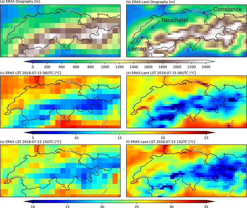
J. Muñoz-Sabater et al.: ERA5-Land                                                                                              4351

parison as it was only available until 2010, and it was in-           puted (Muñoz-Sabater, 2019b). Figure 2 shows a diagram of
tended to be a research dataset. As a reference for the evalua-       the algorithm used for each 24 h production cycle. The most
tion, in situ observations from different networks around the         important components of the production algorithm are pre-
globe have been used for comparison to the reanalyses esti-           sented in the following subsections.
mates. In addition, complementary global gridded model- or
satellite-based datasets have been incorporated into the eval-        2.1   Initialization
uation exercise. Improvements in ERA5 compared to ERA-
Interim are mainly due to 10 years of additional research             ERA5-Land is not produced as a single continuous simula-
and development (R&D) in the use of satellite data in nu-             tion for the entire period. The production is conducted in
merical weather prediction (NWP) and atmospheric mod-                 three independent streams, as shown in Fig. 1. To avoid or
elling (Hersbach et al., 2020). Differences between ERA5              minimize discontinuities between streams, a careful initial-
and ERA5-Land are not so obvious. They both share quite               ization procedure is needed for each of them. Particular at-
similar parameterizations of land processes; the main im-             tention must be given to variables carrying long memory. As
provement of ERA5-Land is due to the non-linear dynamical             an example, Fig. 3 shows time series of deep soil moisture in
downscaling with corrected thermodynamic input.                       a band of latitude between 60 and 20◦ S, where the averaged
   Section 2 describes the main steps of the methodology              annual soil moisture variability is low. This period includes
used to produce ERA5-Land; in Sect. 3, the data used to in-           several production streams of ERA5. ERA5 initialized each
vestigate the added value of ERA5-Land compared to ERA5               stream with ERA-Interim soil moisture initial conditions,
and ERA-Interim (mainly from the years 2000–2018) are de-             which has a different climatology than ERA5. In ERA5, a
scribed. Section 4 shows the results of the evaluation exer-          1-year spin-up was used for each production stream and it is
cise, while information on access to the data is presented in         normally long enough for atmospheric variables. However,
Sect. 5. A discussion of the results and the conclusions is pre-      it is not sufficient for deep soil moisture to reach equilib-
sented in Sect. 6, followed by perspectives for future updates        rium, which leads to discontinuities between two production
in Sect. 7                                                            streams, as shown in Fig. 3.
                                                                         The strategy followed to initialize the ERA5-Land produc-
                                                                      tion stream starting in 2001 (stream-1) was to use the latest
2   Methodology                                                       year of a long, prior ERA5 stream, and letting 3 further spin-
                                                                      up years to allow a long spin-up period (see Fig. 1). While
ERA5-Land produces a total of 50 variables describing the             this strategy provides satisfactory results for most continen-
water and energy cycles over land, globally, hourly, and at a         tal masses around the world, discontinuities are still possible
spatial resolution of 9 km, matching the ECMWF triangular–            at areas with very low variability of soil moisture (deserts and
cubic–octahedral (TCo1279) operational grid (Malardel                 polar regions). Particular attention was given to the treatment
et al., 2016). For a full list of the available fields in the ERA5-   of permanent snow-covered regions. The current model for-
Land catalogue, see Table A2 in Appendix A. The production            mulation (as in ERA5) does not have an independent treat-
is conducted in three segments or streams. The reason is two-         ment of glaciers. Grid points with glaciers are assigned with
fold: (1) it allows the production of parallel streams, there-        a constant snow mass of 10 m. ERA5-Land streams are ini-
fore accelerating the production and the public availability          tialized on the 1 January, and a glacier mask is applied to
of the data; (2) the atmospheric forcing necessary to produce         snow mass to guarantee the correct spatial representation of
ERA5-Land is derived from ERA5, and thus the production               glaciers. A threshold of 50 % of a grid box covered by ice
needs the corresponding segment of ERA5 completed for the             is used, below which the snow depth keeps the value com-
same time period. Figure 1 shows the different data streams           puted by the snow scheme of the land model. Values above
designed in the production of ERA5-Land. The production               the threshold assign a snow water equivalent value of 10 m.
started with data from the year 2001 (stream-1) aiming at             This condition is used to avoid grid points near glaciers with
making available firstly the most recent data, while the back         large unrealistic snow depth that result from the interpola-
extension from 1950 to 1980 (stream-3) is currently under             tion from ERA5 fields to ERA5-Land. For the stream start-
production.                                                           ing in 1981 (stream-2), a long, prior ERA5 stream was not
   Each segment or stream is initialized with meteorologi-            available. The strategy in this case was to initialize using a
cal fields from ERA5. ERA5-Land does not assimilate ob-               ERA5-Land climatology of 1 January for the period 2001–
servations directly. The observations influence the land sur-         2018 and then allow the system to spin up for 3 years. A
face evolution via the atmospheric forcing. Forcing air tem-          similar strategy was used to initialize the stream starting in
perature, humidity, and pressure are corrected using a daily          1950 (stream-3), but in this case a 1981–2010 climatology
lapse rate derived from ERA5. After that, the land surface            was used and only 1 spin-up year was feasible. The latter
model is integrated in 24 h cycles providing the evolution of         was limited by the availability of forcing data.
the land surface state and associated water and energy fluxes.
In addition to the hourly data, monthly means are also com-

https://doi.org/10.5194/essd-13-4349-2021                                             Earth Syst. Sci. Data, 13, 4349–4383, 2021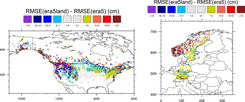
4352                                                                                               J. Muñoz-Sabater et al.: ERA5-Land

Figure 1. Diagram of the production streams of ERA5-Land. The dark blue lines correspond to the data that have already been produced and
are available through the C3S Climate Data Store. The light blue line corresponds to the back-extension period, and at the time of writing this
paper is under production. The 3-year spin-up period for stream-1 and stream-2 is presented with dashed rectangles. Stream-3 has a 1-year
spin-up (1949). The red diamond presents the end of each stream.

Figure 2. Diagram of the algorithm used in the production of ERA5-Land. The land surface model is integrated in 24 h cycles using short-
forecast meteorological forcing fields from ERA5.

2.2    Static and climatological fields                                   2.3   Atmospheric forcing
As in ERA5, the land characteristics are described using sev-
eral time-invariant fields. These consist of the land–sea mask,           ERA5-Land is driven by atmospheric forcing derived from
the lake cover and depth, the soil and vegetation type, and the           ERA5 near-surface meteorology state and flux fields. The
vegetation cover. In addition, surface albedo and leaf area in-           meteorological state fields are obtained from the lowest
dex are prescribed as monthly climatologies. The complete                 ERA5 model level (level 137), which is 10 m above the sur-
list of time invariant fields with their information source is            face, and include air temperature, specific humidity, wind
provided in Table A1 of Appendix A.                                       speed, and surface pressure. The surface fluxes include
                                                                          downward shortwave and longwave radiation and liquid and
                                                                          solid total precipitation. These fields are interpolated from
                                                                          the ERA5 resolution of about 31 km to ERA5-Land resolu-
                                                                          tion of about 9 km via a linear interpolation method based on

Earth Syst. Sci. Data, 13, 4349–4383, 2021                                                  https://doi.org/10.5194/essd-13-4349-2021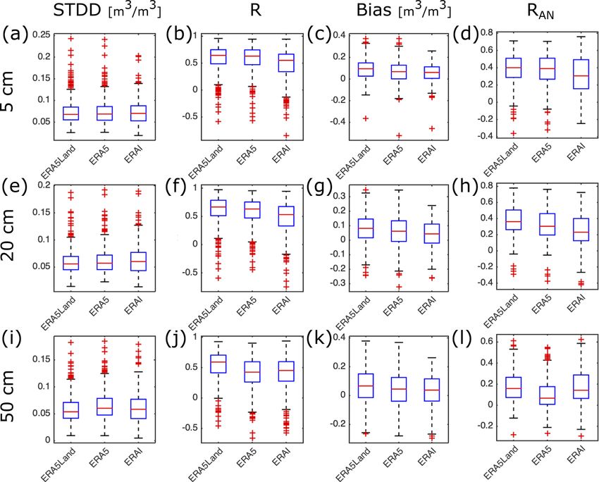
J. Muñoz-Sabater et al.: ERA5-Land                                                                                                    4353

Figure 3. (a) Mean differences between ERA5-Land and ERA5 soil moisture (sm) time series for the fourth soil layer of the Carbon
Hydrology-Tiled ECMWF Scheme for Surface Exchanges over Land (CHTESSEL) land surface model (100–289 cm), averaged for the
latitudes 60–20◦ S. The temporal resolution is 12 h. Panel (b) is the same as (a) but showing the raw time series of ERA5 (dashed light grey
curve) and ERA5-Land (dark curve).

a triangular mesh. The atmospheric forcing built for ERA5-              tion. Taking into account these orographic differences is im-
Land is hourly and consistent over the entire production pe-            portant for other land variables such as surface temperature.
riod, and it is the result of the assimilation of a large num-          For instance, the middle and bottom rows show a more re-
ber of conventional meteorological and satellite observations           alistic spatial pattern of surface temperature in ERA5-Land,
through a four-dimensional variational assimilation system              with a clear cold signal over the higher peaks. It is also re-
(4D-Var) and simplified extended Kalman filter (SEKF) sys-              markable to see how ERA5-Land is able to resolve lakes such
tems as described in Hersbach et al. (2020). Previous land re-          as Geneva (Léman), Neuchâtel, and Constance. This is espe-
analyses have included corrections to the precipitation forc-           cially visible at 06:00 UTC, when the lake surface tempera-
ing to address limitations of the precipitation fields of the           ture is still significantly warmer than the land (Fig. 4f).
atmospheric reanalysis. This is not the case in ERA5-Land
mainly due to the (1) enhanced quality of ERA5 precipita-               2.4    Land surface model
tion when compared with previous atmospheric reanalyses
(e.g. Beck et al., 2019; Tarek et al., 2020; Nogueira, 2020)            The core of ERA5-Land is the ECMWF land surface model:
and (2) reduced dependencies on external data that would                the Carbon Hydrology-Tiled ECMWF Scheme for Surface
limit the near-real-time data availability. However, air tem-           Exchanges over Land (CHTESSEL). The main updates with
perature, humidity, and pressure are corrected for the altitude         respect to the land component of ERA-Interim are (a) a re-
differences between ERA5 and ERA5-Land grids. This cor-                 vised soil hydrology, introducing an improved formulation of
rection involves four steps: (i) relative humidity is computed          the soil hydrologic conductivity and diffusivity (that now is
from interpolated, uncorrected fields; (ii) air temperature is          variable as a function of soil texture) and surface runoff based
adjusted for the altitude differences using a daily environ-            on variable infiltration capacity (Balsamo et al., 2010); (b) a
mental lapse rate (ELR) field derived from ERA5 lower tro-              fully revised parametrization of the snow scheme, changing
posphere temperature vertical profiles (Dutra et al., 2020);            the hydrological and radiative properties of the snowpack
(iii) surface pressure is corrected for the altitude differences        (Dutra et al., 2010); (c) the introduction of a climatologi-
and correction of temperature; and (iv) specific humidity is            cal seasonality of vegetation, in contrast to the fixed vege-
computed using the corrected temperature and pressure as-               tation in ERA-Interim (Boussetta et al., 2013b); (d) a new
suming that there is no change in relative humidity. Dutra              scheme for bare soil evaporation, allowing soil moisture to
et al. (2020) present a detailed evaluation of this methodol-           reach values below the wilting point (Albergel et al., 2012);
ogy comparing the use of a constant (time and space) ELR                (e) introduction of a lake model to represent the thermody-
with daily ELR fields derived from ERA5. This methodol-                 namics of inland water bodies (Balsamo et al., 2012); and
ogy was shown to reduce the mean absolute error (MAE)                   (f) a parametrization that allows the estimation of land carbon
of daily maximum temperature by 10 % and by 4 % for daily               fluxes – net ecosystem exchange (NEE), gross primary pro-
minimum temperature with respect to ERA5 when compared                  duction (GPP), and ecosystem respiration (Reco ) – in a mod-
with 2941 stations over the western US. The importance of               ular way with the Jarvis approach that computes the stomatal
the ELR correction is shown in the orography map of the                 conductance without affecting the transpiration components
Alpine region around Switzerland in Fig. 4. ERA5 misses                 (Boussetta et al., 2013a).
many of the highest Alpine peaks due to the coarser resolu-                The land surface model version used in ERA5-Land
                                                                        was operational at ECMWF in 2018 with the model cycle

https://doi.org/10.5194/essd-13-4349-2021                                                Earth Syst. Sci. Data, 13, 4349–4383, 2021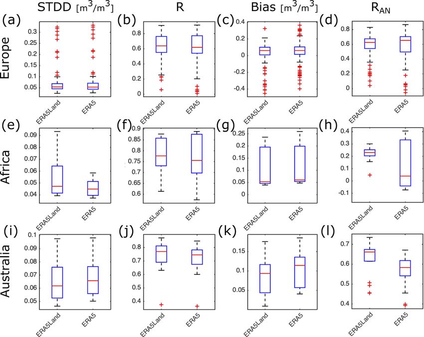
4354                                                                                          J. Muñoz-Sabater et al.: ERA5-Land

Figure 4. ERA5 (a, c, e) and ERA5-Land (b, d, f) orography (a, b) of the Alpine region around Switzerland. Panels (c, d) and (e, f) show
the ERA5 and ERA5-Land land surface temperature (LST) estimates on 15 July 2018 at 06:00 UTC (c, d) and 15:00 UTC (e, f), respectively.
The locations of lakes Geneva (Léman), Neuchâtel, and Constance are indicated in panel (b).

Cy45r1. A detailed description of the model can be found              an estimate of irrigation requirements, one has to be cautious
in chapter IV of the Integrated Forecasting System (IFS)              especially for arid conditions, since the method can give un-
documentation (https://www.ecmwf.int/node/18714, last ac-             realistic results due to too-strong evaporation forced by dry
cess: December 2020). Compared with the model version of              air.
ERA5, the differences are mostly technical, with the excep-
tion of (i) an updated parametrization of the soil thermal con-       3   Data and evaluation strategy
ductivity following Peters-Lidard et al. (1998) that takes into
account the ice component in the case of frozen soil, (ii) a          To evaluate the quality of the ERA5-Land fields, several key
fix to improve conservation for the soil water balance, and           variables of the water and energy cycles were selected and
(iii) rain over snow is accounted for and it does not accumu-         compared to available in situ observations and to a series of
late in the snowpack. Potential evapotranspiration (PET) flux         reference datasets. Note that the list of evaluated variables
in ERA5 suffers from a bug present in IFS cycle 41r2 that             and reference datasets is not exhaustive and was based on
affects PET computation over forests and deserts. This prob-          factors such as availability of data at the time of the evalu-
lem has been corrected in ERA5-Land, and unlike in ERA5,              ation. ERA-Interim and ERA5 reanalyses were included in
ERA5-Land includes PET in the portfolio of products. Given            the comparison, aiming at showcasing the progress of oper-
the importance of this variable for some applications, it is          ational reanalyses at ECMWF. The variables evaluated are
worth clarifying that PET is computed by making a second              soil moisture, snow depth, lake surface water temperature
call to the surface energy balance assuming a vegetation type         and river discharge for the water cycle, the sensible and la-
of crops and no soil moisture stress. In other words, evapora-        tent heat fluxes (the latter also a component of the water cy-
tion is computed for agricultural land as if it is well watered       cle), the Bowen ratio, and skin temperature for the energy
and assuming that the atmosphere is not affected by this arti-        cycle. This section describes the supporting datasets used in
ficial surface condition. The latter may not always be realis-        the evaluation exercise and the metrics employed to assess
tic. Therefore, despite the fact that PET is meant to provide         the quality of ERA5-Land fields.

Earth Syst. Sci. Data, 13, 4349–4383, 2021                                             https://doi.org/10.5194/essd-13-4349-2021
J. Muñoz-Sabater et al.: ERA5-Land                                                                                           4355

3.1   ERA-Interim                                                  two-dimensional optimal interpolation scheme for the anal-
                                                                   ysis of screen-level 2 m temperature and relative humidity,
ERA-Interim (Dee et al., 2011) is the former ECMWF                 and for snow (depth and density), a point-wise simplified ex-
reanalysis providing estimates for the atmosphere, ocean           tended Kalman filter (de Rosnay et al., 2013) for three soil
waves, and land surface. It had supported scientific progress      moisture layers in the top 1 m of soil, and a one-dimensional
during the previous decade and is still widely used today by       optimal interpolation for soil, ice, and snow temperature. De-
the scientific community. It includes information on mul-          tails of the ERA5 configuration are given in Hersbach et al.
tiple land and atmospheric variables, and it is available          (2020), which also contains a basic evaluation of charac-
from January 1979 to August 2019. It used the IFS ver-             teristics and performance for the segment from 1979 on-
sion Cy31r2 (more detailed information available at https:         ward. The performance of the component from 1950 to 1978,
//www.ecmwf.int/en/publications/ifs-documentation, last ac-        the back extension which was made available later, is de-
cess: 27 August 2021), corresponding to the IFS 2006 re-           scribed in Bell et al. (2021), and a detailed analysis for
lease, with a spatial horizontal resolution of about 80 km and     surface temperature and humidity is provided by Simmons
60 levels in the vertical from the surface to 0.1 hPa. The sys-    et al. (2021). Technical details are also provided in the online
tem includes a 4D-Var system (Rabier et al., 2000) providing       documentation (https://confluence.ecmwf.int/display/CKB/
analyses fields at a temporal resolution of 6 and 3 h for short-   ERA5:+data+documentation, last access: 23 August 2021).
forecast fields (like for precipitation and fluxes). The main         Both ERA5 and ERA5-Land are produced as part of the
difference between the land component of ERA-Interim and           Copernicus Climate Change Service that ECMWF operates
those of both ERA5 and ERA5-Land is that the former is             on behalf of the European Commission and are available
based on TESSEL (van den Hurk et al., 2000), which is con-         from the C3S Climate Data Store (CDS). ERA5 and ERA5-
sidered the precursor of the current CHTESSEL scheme. In           Land have a large and diverse user base (more than 40 000
ERA-Interim, the soil moisture and soil temperature analyses       users at the end of 2020). Table 1 summarizes the main char-
are based on a local optimal interpolation scheme (Mahfouf,        acteristics of ERA-Interim, ERA5, and ERA5-Land.
1991; Douville et al., 2000) that assimilates surface synoptic
(SYNOP) observations of temperature and relative humidity
at screen level (2 m). The snow depth analysis is indepen-         3.3   Soil moisture
dent of the soil wetness and is based on a Cressman analysis       To evaluate the quality of the soil moisture estimates from
that assimilates SYNOP snow reports and snow-free satellite        the various reanalyses, a large number (> 800) of in situ
observations (Drusch et al., 2004).                                sensors in the period 2010 to 2018, many providing hourly
                                                                   measurements, were used. These sensors belong to the net-
3.2   ERA5                                                         works that are listed in Table 2. The networks are located
                                                                   in North America, Europe, Africa, and Australia, and all
ERA5 is the latest comprehensive ECMWF reanalysis and              the observations were retrieved from the International Soil
has replaced ERA-Interim. It is based on a version of the          Moisture Network (Dorigo et al., 2011, 2021). Three reanal-
ECMWF IFS (Cy41r2) that was operational in 2016. ERA5              ysis soil layer estimates were compared to measurements by
provides hourly estimates of the global atmosphere, land sur-      sensors at three different depths. ERA5 and ERA5-Land top
face, and ocean waves from 1950 and is updated daily with          layer soil moisture estimates (0–7 cm) were compared to in
a latency of 5 d. Its state estimates are based on a high-         situ sensors at 5 cm depth in North America, Africa, Eu-
resolution (HRES) component at a horizontal resolution of          rope, and Australia. A more in-depth study was performed
31 km and with 137 levels in the vertical spanning from the        in North America, where most of the sensors are located.
surface up to 0.01 hPa. Information on uncertainties in these      For this region, surface soil moisture from ERA-Interim was
are provided by a 10-member ensemble of data assimila-             also evaluated. In addition, ERA5, ERA5-Land, and ERA-
tions (EDA) at half the horizontal resolution. Both the HRES       Interim soil moisture for the second (7–28 cm) and third lay-
and EDA ERA5 data assimilation use background-error es-            ers (28–100 cm) were evaluated against in situ measurements
timates that utilize the output from the EDA. The land com-        at 20 and 50 cm depth, respectively. In situ measurements
ponent of ERA5 is, like ERA5-Land, based on the CHTES-             were compared to the closest grid point of the ERA5, ERA5-
SEL model, though at a resolution of 31 km rather than 9 km.       Land, and ERA-Interim grids if the closest grid point was
ERA5 uses new analyses of sea-surface temperature and sea-         not farther than the respective model resolution. In situ time
ice concentration, variations in radiative forcing derived from    samples were selected in a ±1 h window with respect to the
CMIP5 specifications, and various new and reprocessed ob-          reanalysis timestamp. If several observations were retrieved
servational data records.                                          in a single window, the average was computed. In order to
   The data assimilation system consists of an incremental         consider an observed time series suited for the comparison,
4D-Var component (Courtier et al., 1994) for upper-air and         a minimum of 150 samples was required for the study pe-
near-surface components, an ocean-wave optimal interpola-          riod. To remove the seasonal cycle, anomaly time series were
tion scheme, and a dedicated LDAS. The LDAS comprises a            also computed. The soil moisture anomaly values at time

https://doi.org/10.5194/essd-13-4349-2021                                         Earth Syst. Sci. Data, 13, 4349–4383, 2021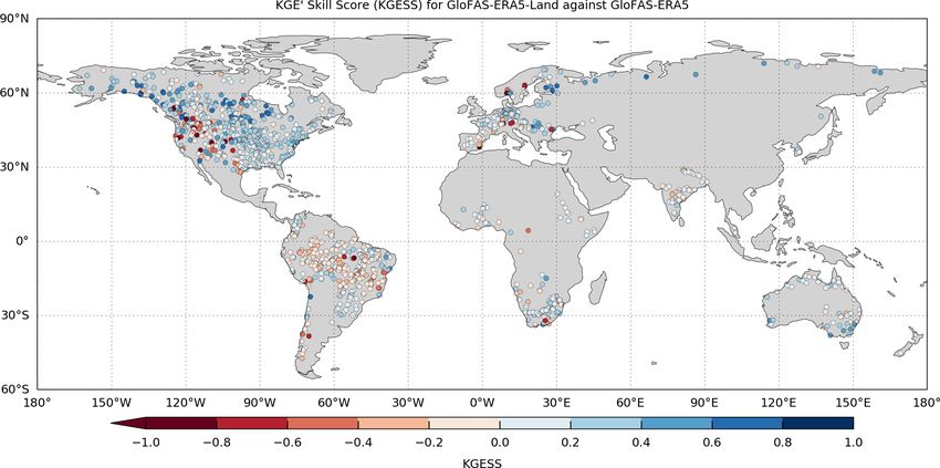
4356                                                                                                                   J. Muñoz-Sabater et al.: ERA5-Land

Table 1. Overview of the main characteristics of ERA-Interim, ERA5, and ERA5-Land.

                                                    ERA-Interim                     ERA5                               ERA5-Land
         Period publicly available∗                 1979–Aug 2019                   1950 onwards                       1981 onwards
                                                                                                                       (1950–1980, in 2021)
         Spatial resolution                         79 km/60 levels                 31 km/137 levels                   9 km
         Land surface model                         IFS (+ TESSEL)                  IFS (+ CHTESSEL)                   CHTESSEL
         Model cycle (year)                         Cy31r2 (2006)                   Cy41r2 (2016)                      Cy45r1 (2018)
         Output frequency                           6-hourly (analyses)             Hourly                             Hourly
                                                    3-hourly (forecasts)
         Uncertainty estimate                       None                            Based on a 10-member 4D-Var        As for ERA5
                                                                                    ensemble at 63 km
         Availability behind real time              n/a                             2–3 months (final product)         2–3 months (final product)
                                                                                    5 d (preliminary product)          5 d (preliminary product, in 2021)
       ∗ Availability at the time of submitting this paper. n/a – not applicable.

t (SMAN (t)) were computed from the original time series                                     eraged snow depth estimates from ERA-Interim, ERA5, and
(SM(t)) computing the mean (SM) and the standard devia-                                      ERA5-Land at 00:00 and 12:00 UTC. To compare the reanal-
tion (σSM ) of soil moisture a ±17 d window as follows:                                      ysis data with the snow depth observations, the prognostic
                                                                                             snow water equivalent (SWE, in units of m water equivalent)
                SM(t) − SM                                                                   and snow density (ρsnow , kg m−3 ) from the reanalysis were
SMAN (t) =                 .                                                        (1)
                   σSM                                                                       combined to compute the actual snow depth (SD, m):
   The following metrics were computed between the reanal-                                                  SWE
yses estimates and the in situ time series: the standard de-                                 SD = ρwater          ,                                         (2)
                                                                                                            ρsnow
viation of the difference (STDD, equivalent to the unbiased
RMSD), the bias, and the Pearson correlation coefficient (R).                                where ρwater = 1000 kg m−3 is the reference density of the
The latter was also computed for the anomaly time series                                     water. The GHCN observations were only considered if snow
(RAN ). The results were grouped per continent and their dis-                                depth values were positive and missing values were lower
tribution presented in box plots. Values are considered out-                                 than 50 % of the recorded time series. Also stations where
liers if they are greater than q75 + 1.5 × (q75 − q25 ) or less                              the snow depth reported is lower than 1 cm in more than 5 %
than q25 − 1.5 × (q75 − q25 ), with q25 and q75 the 25th and                                 of the total number of days were removed. Finally, stations
75th percentiles, respectively.                                                              located in coastal areas with more than 50 % water in the
                                                                                             pixel and on permanent snow area (glaciers) were removed.
3.4    Snow                                                                                  More than 6000 stations passed the quality filters, and their
                                                                                             locations can be found in Fig. 9. The quality of the snow
Snow depth estimates from reanalyses were compared to two                                    depth from the reanalyses was evaluated at the hemispheric
sets of observational data. The first one comprises 10 sites                                 scale by computing the mean bias (here defined as reanalysis
distributed among North America, Europe, and Japan. They                                     estimate minus in situ observation) and root mean square er-
were selected as reference sites to evaluate cold processes                                  ror (RMSE) for the months between December and June of
by models participating in the Earth System Model – Snow                                     the 2010–2018 period.
Model Intercomparison Project (ESM-SnowMIP) (Krinner
et al., 2018; Ménard et al., 2019). These sites provide bench-
                                                                                             3.5    Lakes
marking data for cold processes in maritime, Alpine, and
taiga types of snow cover and on different types of climates.                                In 2015, the CHTESSEL land surface scheme of the oper-
Table 3 presents these stations.                                                             ational IFS introduced a lake tile, which represents lakes,
   The second dataset is retrieved from the Global Historical                                reservoirs, rivers, and coastal (subgrid) waters, and is based
Climatology Network-Daily (GHCN-daily) (Menne et al.,                                        on the FLake (Fresh-water Lake) model of Mironov et al.
2012b) from 1 July 2010 to 30 June 2018. The version used                                    (2010a). FLake is a one-dimensional model, which uses an
is v3.24 (Menne et al., 2012a). This network integrates thou-                                assumed shape for the lake temperature profile including the
sands of land surface stations across the globe. The daily ob-                               mixed layer (uniform distribution of temperature) and the
served snow depth product was compared to the daily av-                                      thermocline (its upper boundary located at the mixed-layer

Earth Syst. Sci. Data, 13, 4349–4383, 2021                                                                       https://doi.org/10.5194/essd-13-4349-2021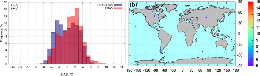
J. Muñoz-Sabater et al.: ERA5-Land                                                                                                   4357

Table 2. In situ measurement networks used to evaluate soil moisture. The different columns contain the region and the name of the network,
the depths of the probes used, and the bibliographic reference to the network.

              Network            Region             Sensor depth    Number of         Reference
                                                    used (cm)       sensors used
                                                                    at each depth
              SCAN               North America      5, 20, 50       185, 189, 190     Schaefer et al. (2007)
              USCRN              North America      5, 20, 50       98, 75, 75        Bell et al. (2013)
              SNOTEL             North America      5, 20, 50       290, 300, 297     Leavesley et al. (2008)
              SOILSCAPE          North America      5, 20           94, 74            Moghaddam et al. (2010b)
              TERENO             Europe             5               10                Zacharias et al. (2011)
              SMOSMANIA          Europe             5               21                Calvet et al. (2007)
              FMI                Europe             5               8                 Ikonen et al. (2016)
              Remedhus           Europe             5               22                Martínez-Fernández and Ceballos (2005)
              Oracle             Europe             5               5                 Tallec et al. (2015)
              VAS                Europe             5               2                 Lopez-Baeza et al. (2009)
              HOBE               Europe             5               39                Bircher et al. (2012)
              AMMA-Catch         Africa             5               9                 Lafore et al. (2010)
              DAHRA              Africa             5               1                 Tagesson et al. (2015)
              Oznet              Australia          5               19                Young et al. (2008), Smith et al. (2012)

Table 3. List of ESM-SnowMIP sites used for the evaluation of the snow parameters, adapted from Krinner et al. (2018).

                 Station               Short name     Years          Biome            Elevation (m)   Coordinates
                 Col de Porte          cdp            1994–2014      Alpine                   1325    45.30◦ N, 5.77◦ E
                 Reynolds Mt. East     rme            1988–2008      Alpine                   2060    43.06◦ N, 116.75◦ W
                 Weissfluhjoch         wfj            1996–2016      Alpine                   2540    46.83◦ N, 9.81◦ E
                 Swamp Angel           swa            2005–2015      Alpine                   3371    37.91◦ N, 107.71◦ W
                 Senator Beck          snb            1995–2015      Alpine                   3714    37.91◦ N, 107.73◦ W
                 Sapporo               sap            2005–2015      Maritime                   15    43.08◦ N, 141.34◦ E
                 Sodankylä             sod            2007–2014      Arctic                    179    67.37◦ N, 26.63◦ E
                 Old Aspen             oas            1997–2010      Boreal forest             600    53.63◦ N, 106.20◦ W
                 Old Black Spruce      obs            1997–2010      Boreal forest             629    53.99◦ N, 105.12◦ W
                 Old Jack Pine         ojp            1997–2010      Boreal forest             579    53.92◦ N, 104.69◦ W

bottom, and the lower boundary at the lake bottom). To run                       and 2018. In addition, daily averaged values were also
FLake, the lake location (or fractional cover), lake depth                       computed.
(most important parameter, preferably bathymetry), and lake
                                                                             – In total, 27 Finnish lakes monitored by Finnish Environ-
initial conditions are required. For the best performance, lake
                                                                               ment Institute (SYKE) provided daily data (one mea-
depth should be updated with the latest available information
                                                                               surement per day at 08:00 LT) from 2000 to 2016. In
to ensure that depths are close to observed values, as over-
                                                                               addition, summer month (June, July, and August) aver-
estimated depths can be blamed for cold biases in summer
                                                                               age values were calculated.
temperatures or lack of ice. The state of lakes in FLake is de-
scribed by seven prognostic variables: mixed-layer tempera-                  – Summer month average values were provided from
ture, mixed-layer depth, bottom temperature, mean temper-                      the global inventory “Globally distributed LSWT
ature of the water column, shape factor (with respect to the                   collected in situ and by satellites; 1985–2009”
temperature profile in the thermocline), temperature at the ice                (https://portal.edirepository.org/nis/mapbrowse?
upper surface, and ice thickness. In this paper, the lake sur-                 packageid=knb-lter-ntl.10001.3, last access: 29 Au-
face water temperature (LSWT) estimates from the FLake                         gust 2021). In total, there were 348 lakes over the globe
model embedded in ERA5 and ERA5-Land were compared                             with in situ data for 15 years (1995–2009).
to in situ observations from three different sources of data,
                                                                         Figure 5 provides the location of all the sources of in situ
during ice-free periods:
                                                                         data used in this study. Considering the above observations
  – The Alqueva reservoir in Portugal, from the Portuguese               as the truth, the MAE of ERA5 and ERA5-Land LSWT es-
    University of Évora, provided hourly data from 2017                  timates was computed. The significance of these results was

https://doi.org/10.5194/essd-13-4349-2021                                                 Earth Syst. Sci. Data, 13, 4349–4383, 2021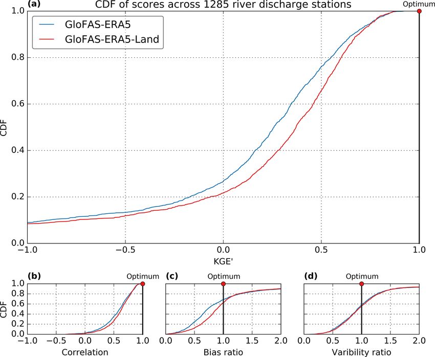
4358                                                                                        J. Muñoz-Sabater et al.: ERA5-Land

tested using the Kruskal–Wallis test by ranks. In addition,       series monitoring an artificial canal instead of a river). This
the bias distribution was also calculated and presented in 2-     filtering procedure resulted in the selection of 1285 stations
D bar graphs. It should be noted that the Alqueva reservoir       with drainage areas ranging between 575 and 4 664 200 km2 ,
and the 27 Finnish lake depths were verified (in situ vs. op-     and a median of 29 963 km2 . Following the methodology of
erational values) and are in good agreement; the lake depths      Harrigan et al. (2020), hydrological performance was as-
provided by the “Globally distributed LSWT collected in situ      sessed using the modified Kling–Gupta efficiency (KGE0 )
and by satellites; 1985–2009” global inventory were only          metric (Gupta et al., 2009; Kling et al., 2012). The KGE0 is
randomly verified (e.g. by comparison with scientific publi-      an overall summary measure consisting of three components
cations), which might add some uncertainty when interpret-        important for assessing hydrological dynamics: temporal er-
ing the results.                                                  rors through correlation, bias errors, and variability errors:
                                                                                  q
                                                                        0
3.6    River discharge                                            KGE = 1 − (R − 1)2 − (β − 1)2 − (γ − 1)2                    (3)
The current version of CHTESSEL does not directly pro-               µs            σs /µs
                                                                  β=            γ=        ,                                   (4)
duce river discharge at the river basin scale. Instead, grid-        µo            σo /µo
ded surface and subsurface runoff from CHTESSEL is cou-
pled to the LISFLOOD hydrological and channel routing             where R is the Pearson correlation coefficient between re-
model (Van Der Knijff et al., 2010). Coupling ERA5/ERA5-          analysis simulations (s) and observations (o), β is the bias
Land runoff with LISFLOOD allows for lateral connectiv-           ratio, γ is the variability ratio, µ the mean discharge, and σ
ity of grid cells with runoff routed through the river chan-      the discharge standard deviation. The KGE0 and its three de-
nel to produce river discharge (m3 s−1 ). This is the process     composed components (correlation, bias ratio, and variabil-
used within the Global Flood Awareness System (GloFAS;            ity ratio) are all dimensionless, with an optimum value of 1.
https://www.globalfloods.eu/, last access: 29 August 2021).       To evaluate the hydrological skill of GloFAS-ERA5-Land,
More details can be found in Harrigan et al. (2020). River        the KGE0 can be computed as a skill score, KGESS, with
discharge estimates from ERA5 (GloFAS-ERA5) and ERA5-             GloFAS-ERA5 used as the benchmark:
Land (GloFAS-ERA5-Land) were obtained for the period                             KGE0GloFAS−ERA5-Land − KGE0GloFAS−ERA5
January 2001 to December 2018. This is the common period          KGESS =                                               , (5)
                                                                                       KGE0perf − KGE0GloFAS−ERA5
for which reanalysis data were available at the time of this
study. Estimates were resampled to the GloFAS 0.1◦ grid-
ded river network at a daily time step. As part of GloFAS,        where KGE0GloFAS−ERA5-Land is the KGE0 value for
a database of global hydrological observations for 2042 sta-      the GloFAS-ERA5-Land reanalysis against observations,
tions is held, consisting predominantly (i.e. ∼ 75 %) of the      KGE0GloFAS−ERA5 is the KGE0 value for the GloFAS-ERA5
Global Runoff Data Centre (GRDC) and supplemented by              benchmark against observations, and KGE0perf is the value
data collected through collaboration with GloFAS partners         of KGE0 for a perfect simulation, which is 1. KGESS =
worldwide to improve spatial coverage. The locations of the       0 means the GloFAS-ERA5-Land reanalysis is no better
stations have been matched to the corresponding cells on the      than the GloFAS-ERA5 benchmark and thus has no skill,
0.1◦ GloFAS river network. Following Harrigan et al. (2020),      KGESS > 0 indicates when GloFAS-ERA5-Land is consid-
a number of criteria were used to select stations for the eval-   ered skilful, and KGESS < 0 is when the performance is
uation:                                                           worse than the GloFAS-ERA5 benchmark.

  – at least 4 years of data available between 2001 and 2018
                                                                  3.7       Energy fluxes
    (not necessarily contiguous),
                                                                  3.7.1      FLUXNET data
  – minimum upstream area of 500 km2 ,
                                                                  The evaluation of the ERA5-Land turbulent fluxes estimates
  – difference in catchment area supplied by the data             was conducted mostly following the method of Martens et al.
    provider and upstream area for the corresponding cell         (2020). Surface sensible and latent heat fluxes (also denoted
    on the GloFAS river network must be within 20 %, and          in this paper as H and λρE, respectively) derived from
  – station with the longest record retained when multiple        ERA reanalyses, as well as their ratio (i.e. the Bowen ra-
    observation stations were matched to the same GloFAS          tio, hereafter denoted as β), were compared to measurements
    river cell.                                                   from the FLUXNET 2015 synthesis dataset (Pastorello et al.,
                                                                  2020). The period under evaluation was based on the avail-
In addition to the above conditions, a first-order visual qual-   ability of reanalysis data at the time of the comparison, and
ity check on observed river discharge time series removed         therefore, unlike in Martens et al. (2020), the evaluation pe-
stations with erroneous data (for example, time series trun-      riod is constrained to 2001–2014. Following Martens et al.
cated above a threshold, showing several inhomogeneities or       (2017), the in situ flux data were subjected to quality control,

Earth Syst. Sci. Data, 13, 4349–4383, 2021                                            https://doi.org/10.5194/essd-13-4349-2021
J. Muñoz-Sabater et al.: ERA5-Land 4359
Figure 5. Location of lakes with in situ data used in this study; green dots are for hourly and daily data for the Alqueva reservoir (Portugal),
red for daily and 3-summer-month averaged data (Finnish lakes), blue for the 3-summer-month average data for lakes all over the globe.
including (1) the removal of rainy intervals, during which situ data, were masked using a quantile-based approach. The
eddy-covariance measurements are typically unreliable, and bias, i.e. the difference between raw in situ time series and re-
(2) the removal of gap-filled records to retain only the actual analysis estimates, the standardized MAE, and the anomaly
measurements from the eddy-covariance sites. After quality Pearson correlation coefficient (RAN ) were computed. The
control, only sites with a minimum record of 5 years were results are shown in the form of violin plots in Sect. 4.5.1.
retained too. In total, 65 eddy-covariance sites remained af-
ter quality control and were used as in situ reference data.
Note that the measured energy fluxes used as reference in 3.7.2 GLEAM
this paper were not corrected for energy balance closure be-
cause the number of towers used for validation would be The Global Land Evaporation Amsterdam Model (GLEAM;
drastically reduced, as the ground-heat flux is also needed Miralles et al., 2011; Martens et al., 2017) is used in this
and is not available from many towers. Some authors have study with two objectives: (a) to compare the GLEAM evap-
already highlighted the lack of closure in the energy balance oration estimates directly to the ERA5 and ERA5-Land es-
at eddy-covariance sites and a consequential tendency to un- timates, which in turn will assess the skill of the underly-
derestimate the latent heat flux (Wilson et al., 2002; Ershadi ing land surface model to simulate turbulent heat fluxes, and
et al., 2014; Jiménez et al., 2018). The reference sites are (b) as an intermediate tool to assess the quality differences of
mainly distributed across the continental US, Europe, and key input meteorological drivers of the turbulent fluxes com-
Australia (see their locations in Fig. 17a, b, and c, respec- puted by GLEAM. GLEAM is a process-based, yet semi-
tively). For each eddy-covariance site, the in situ measure- empirical, model that computes total evaporation and its sep-
ments were aggregated from their native temporal resolution arate components over continental masses at global scale. A
to hourly, 3-hourly, and daily intervals. In addition, standard- detailed description of this model can be found in Martens
ized anomalies were calculated by subtracting for each time et al. (2017) and Miralles et al. (2010, 2011). In this pa-
interval the climatological expectation (i.e. the average value per, version 3 (v3) of the GLEAM algorithm is used and
across the entire record for that interval) and dividing by the forced with the same database as in the official v3.4a dataset
standard deviation of that climatology. While the compari- (see https://www.gleam.eu, last access: 29 August 2021),
son to raw time series may mask the influence of short-term including near-surface air temperature and surface net ra-
meteorological anomalies on surface energy partitioning (as diation from ERA5; this dataset is hereafter referred to
the temporal variability of turbulent fluxes typically depends as GLEAM + ERA5. Likewise, a version of GLEAM run
strongly on the seasonality of its main drivers), the compari- with ERA5-Land air temperature and surface net radiation
son to anomaly time series reflects the response to short-term is referred to as GLEAM + ERA5-Land. Analogous com-
meteorological conditions. The Bowen ratio was only calcu- parisons between GLEAM + ERA5 and GLEAM + ERA-
lated at daily temporal resolution for numerical instability Interim (using forcing fields from ERA-Interim) can be
reasons. As described in Martens et al. (2020), outliers in the found in Martens et al. (2020). Surface latent heat flux,
time series of the Bowen ratio, for both the reanalyses and in surface sensible heat flux, and the Bowen ratio from
GLEAM + ERA5 and GLEAM + ERA5-Land were evalu-
https://doi.org/10.5194/essd-13-4349-2021 Earth Syst. Sci. Data, 13, 4349–4383, 20214360 J. Muñoz-Sabater et al.: ERA5-Land
ated against the eddy-covariance data described in Sect. 3.7.1 higher R than ERA5 (both for the original time series and the
at daily timescales. anomaly times series). The evaluation obtained over Europe,
Africa, and Australia shows an overall slightly better perfor-
3.8 Skin temperature
mance of ERA5-Land over ERA5; in particular, the anomaly
correlation of the top layer is improved predominantly in the
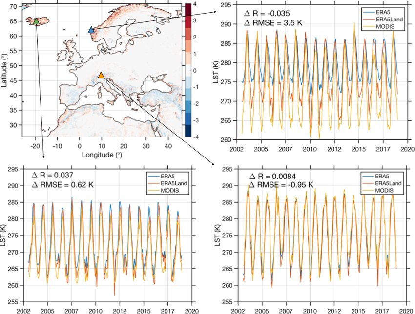
The skin temperature is the theoretical temperature of the warmest climates. Nonetheless, these results for the top soil
Earth’s surface that is required to satisfy the surface en- layer are not conclusive, partly because of the insufficient
ergy balance. It represents the temperature of the upper- number of available stations.
most surface layer, which has no heat capacity and thus To get more insight into the soil moisture evaluation,
can respond instantaneously to changes in surface fluxes. ERA5-Land and ERA5 were also evaluated over North
The top surface layer of the ECMWF’s land surface model, America, where most of the in situ sensors are available, in-
CHTESSEL, covers the top 7 cm. In order to evaluate the cluding several hundreds of sensors at 20 and 50 cm depths.
skill of ERA5-Land land surface temperature (LST), NASA’s In addition, the same evaluation was performed for ERA-
Moderate Resolution Imaging Spectroradiometer (MODIS) Interim to address the evolution of ERA5 and ERA5-Land
MYD11C3/MOD11C3 version 6 product was used in this with respect to the previous reanalysis generation. Figure 7
study. It provides monthly LST and emissivity values for shows the evaluation results for ERA5-Land, ERA5, and
Aqua and Terra in a 0.05◦ (5600 m at the Equator) latitude– ERA-Interim soil moisture top three layers against measure-
longitude climate modelling grid (CMG), for day and night ments for sites in North America at 5 cm (Fig. 7a–d), 20 cm
overpasses. Chen et al. (2017) recommended the use of (Fig. 7e–h), and 50 cm depth (Fig. 7i–l). ERA5 and ERA5-
the MODIS LST average ensemble (i.e. from Aqua-day, Land surface soil moisture obtains quite similar results for
Aqua-night, Terra-day, and Terra-night) for climate stud- all the metrics, although the median of the correlation and
ies and reported validation with 156 flux tower measure- anomaly correlation are slightly better in ERA5-Land. ERA-
ments (RMSE = 2.65, mean bias < ±1 K). In this study, the Interim obtains lower values for these last two metrics, mean-
MODIS observational LST ensemble was constructed fol- ing that the land improvements in CHTESSEL compared to
lowing Chen et al. (2017) and used as a reference for com- the old TESSEL scheme lead to better representation of the
parison with ERA-Interim, ERA5, and ERA5-Land monthly soil moisture dynamics. In deeper layers, the performance
averaged LST data for the period January 2003 to Decem- of ERA5-Land is better than that of ERA5, in particular for
ber 2018 (16 years). MODIS data were firstly averaged to the third layer, for which ERA5-Land shows lower STDD
monthly timescales and then upscaled at two spatial resolu- (Fig. 7i) and higher correlation (Fig. 7j, l) than ERA5. It is
tions: to 0.1◦ for comparison to ERA5-Land, and to 0.25◦ for worth mentioning that for the third soil layer of the model,
comparison to ERA5 and ERA-Interim data. Bias, Pearson’s ERA5 performs quite similarly to ERA-Interim, which is
correlation (R), and RMSE were computed on the full time likely due to the initialization of the ERA5 streams with
series, and correlation was also computed on the anomalies ERA-Interim soil moisture conditions.
(RAN ), calculated as departures from the monthly climatol- Finally, the results were also analysed site per site taking
ogy. into account the confidence interval of the Pearson correla-
tion obtained for ERA5 and ERA5-Land versus the in situ
measurements. A correlation difference is considered signif-
4 Evaluation results
icant if the confidence intervals do not overlap. The Pearson
4.1 Soil moisture
correlation difference for ERA5 and ERA5-Land at 5 cm is
significant for 382 sensors, of which 64 % shows higher cor-
Figure 6 shows the evaluation results for ERA5-Land and relation for ERA5-Land. The correlation difference at 20 cm
ERA5 top soil moisture layer against 5 cm depth measure- is significant for 417 sites, of which 72 % show a higher cor-
ments for sites in Europe, Africa, and Australia. For sites relation for ERA5-Land. Finally, the correlation difference
in Europe, both ERA5-Land and ERA5 show similar STDD at 50 cm is significant for 479 sites, of which 88 % show a
and bias distributions (Fig. 6a, c). The distribution of R is higher correlation for ERA5-Land.
also similar but the median value obtained for ERA5-Land is
slightly higher than for ERA5 (Fig. 6b). In contrast, ERA5 4.2 Snow
shows a slightly higher median for the anomaly correlation,
although ERA5-Land shows a more compact distribution Figure 8 shows the mean bias and RMSE of the SWE nor-
(Fig. 6d). In Africa, only 10 sensors at a depth of 5 cm were malized by the mean value and standard deviation of the
available. The STDD shows a larger distribution for ERA5- observations, respectively, for the 10 sites of Table 3. Each
Land (Fig. 6e); however, the latter shows slightly lower bias column displays the statistics of the nearest neighbour point,
and better R (Fig. 6f, g). The anomaly correlation is largely whereas the vertical bars represent the minimum and max-
improved (Fig. 6h). Finally, in Australia, ERA5-Land box imum values of the metrics computed over the four nearest
plots (Fig. 6i–l) clearly show lower STDD and bias, and points. Hence, this enables the characterization of the spatial
Earth Syst. Sci. Data, 13, 4349–4383, 2021 https://doi.org/10.5194/essd-13-4349-2021J. Muñoz-Sabater et al.: ERA5-Land 4361 Figure 6. Box plots showing the evaluation of ERA5-Land and ERA5 top layer soil moisture against in situ measurements at 5 cm for sites in Europe (a–d), Africa (e–h), and Australia (i–l). Panels (a), (e), and (i) show the standard deviation of the difference (STDD), (b), (f), and (j) the Pearson correlation coefficient (R), (c), (g), and (k) the bias, and (d), (h), and (l) the Pearson correlation of the anomaly time series (RAN ). On each box, the central mark indicates the median, and the bottom and top edges of the box indicate the 25th (q25 ) and 75th (q75 ) percentiles, respectively. The whiskers extend to the most extreme data points not considered outliers. variability of the errors given that many sites are located in this site; see time series in Fig. S1 in the Supplement), even complex terrains or coastal area. though the spatial variability is higher in ERA5. On the con- Considering the mountain sites, ERA5-Land shows lower trary, at the forest sites (oas, obs, ojp), snow depth assimila- RMSE over the sites with moderate altitude, i.e. between tion can remove snow mass to compensate for errors in snow 1300 and 2500 m (cdp, rme, wfj). ERA5-Land also clearly density, the latter which are not considered in the assimila- presents the lowest errors in the Arctic site (sod) and in the tion system. Finally, noteworthy are the improvements in the boreal forest sites (oas, obs, and ojp). Overall, the biases are transition between ERA-Interim and ERA5, in particular at smaller in ERA5-Land than in ERA5 (and ERA-Interim) at Sodankylä (sod), which is caused by improved parameteri- these sites. For the mountain sites, all reanalyses are char- zations of the snow model introduced between ERA-Interim acterized by a negative bias, which is very likely due to the and ERA5 productions (Dutra et al., 2010). smoothing of the orography at the resolution of the reanal- Figure 9 shows the maps of the RMSE difference be- ysis. The higher horizontal resolution of ERA5-Land, com- tween ERA5-Land and ERA5 snow depth estimates when pared to ERA5, helps to reduce the bias at cdp, rme, and compared to in situ observations of the GHCN network, for wfj caused by a better orographic representation. However, both North America and Europe. Over the US, and partic- the agreement with in situ observations at the sites located in ularly over the Rockies region, ERA5-Land generally out- very high mountains (snb and swa, located at altitudes greater performs ERA5 in terms of lower RMSE (see Fig. 9a). In than 3300 m) is slightly better with ERA5 than with ERA5- these highly complex terrain regions, the higher horizontal Land. It should be noted that the four nearest grid points indi- resolution of ERA5-Land adds value by providing more real- cate a much larger spread of errors for ERA5 than for ERA5- istic orographic contours. However, over Europe (i.e. mainly Land. Therefore, compensating errors could lead to better Scandinavia; see Fig. 9b), where ERA5 uses a dense SYNOP performance of ERA5 at the nearest grid point. The maritime network of observations in the snow assimilation system, site (sap) also shows lower RMSE in ERA5. At this site, the ERA5 performs better than ERA5-Land. data assimilation can help in adding/removing snow mass for To further quantify the impact of the higher horizontal res- the right reason (snow density is overall well represented at olution of ERA5-Land on snow depth simulation, Fig. 10 https://doi.org/10.5194/essd-13-4349-2021 Earth Syst. Sci. Data, 13, 4349–4383, 2021
You can also read