Experimental Study on Seepage Anisotropy of a Hexagonal Columnar Jointed Rock Mass
←
→
Page content transcription
If your browser does not render page correctly, please read the page content below
Hindawi
Shock and Vibration
Volume 2021, Article ID 6661741, 15 pages
https://doi.org/10.1155/2021/6661741

Research Article
Experimental Study on Seepage Anisotropy of a Hexagonal
Columnar Jointed Rock Mass

          Yanxin He ,1,2 Zhende Zhu,1,2 Wenbin Lu ,1,2 Yuan Tian,1,2 Xinghua Xie,3
          and Sijing Wang1,4
          1
            Key Laboratory of Ministry of Education of Geomechanics and Embankment Engineering, Hohai University,
            Nanjing 210098, China
          2
            Jiangsu Research Center for Geotechnical Engineering, Hohai University, Nanjing 210098, China
          3
            Nanjing Hydraulic Research Institute, Nanjing 210029, China
          4
            Institute of Geology and Geophysics, Chinese Academy of Sciences, Beijing 100029, China

          Correspondence should be addressed to Wenbin Lu; wblhh@hhu.edu.cn

          Received 27 December 2020; Revised 15 January 2021; Accepted 19 January 2021; Published 28 January 2021

          Academic Editor: Guangchao Zhang

          Copyright © 2021 Yanxin He et al. This is an open access article distributed under the Creative Commons Attribution License,
          which permits unrestricted use, distribution, and reproduction in any medium, provided the original work is properly cited.
          Many columnar jointed rock masses (basalt) are present at the Baihetan hydropower dam site, and their seepage characteristics
          have a significant impact on the project’s safety and stability. In this study, model samples consisting of material similar to the
          columnar jointed rock mass with different inclination angles (0°–90°) were prepared and laboratory triaxial seepage tests were
          performed to study the seepage characteristics of the columnar jointed rock mass under maximum axial principal stress. The
          experimental results showed that the similar material model samples of columnar jointed rock mass showed obvious seepage
          anisotropy. The nonlinear seepage characteristics were well described by the Forchheimer and Izbash equations, and the fitting
          coefficients of the two equations were in good correspondence. The curves describing the relationship between the inherent
          permeability and the stress of the samples with different dip angles were U-shaped and L-shaped, and a one-variable cubic
          equation well described the relationship. The 45° angle specimen had the highest sensitivity to the maximum principal stress, and
          its final permeability increased by 144.25% compared with the initial permeability. The research results can provide theoretical
          support for the stability evaluation of the Baihetan hydropower station.

1. Introduction                                                         dominant reasons for large-scale engineering instability and
                                                                        engineering geological disasters [7, 8]. Statistics have shown
A columnar jointed rock mass is formed by rapid cooling                 that more than 90% of rock slope failures are related to
and shrinkage of high-temperature lava. It is a discontin-              groundwater permeability, 60% of coal mine shaft damage is
uous, multiphase, and anisotropic geological body. These                related to groundwater, and 30%–40% of dam failures of
types of rock masses are widely distributed globally. Nu-               water conservancy and hydropower projects are caused by
merous densely developed slender columnar jointed rock                  seepage [9, 10]. Therefore, it is crucial to study the seepage
masses are exposed in the dam foundation and underground                characteristics of columnar jointed rock masses under stress
powerhouse area of the Baihetan hydropower station in                   in water conservancy and hydropower projects for practical
China (Figure 1) [1, 2].                                                engineering applications.
    Current research on columnar jointed rock masses has                    Research on rock mass seepage has mainly focused on the
primarily focused on the mechanical properties and an-                  seepage characteristics of a single joint surface. Louis et al.
isotropic deformation and failure [3–6]. However, numer-                verified the applicability of the cubic law of laminar flow in a
ous practical engineering projects have shown that the                  seepage test of smooth parallel plate fractures [11, 12]. How-
damage and deformation of rock masses and changes in the                ever, the structure of a natural joint surface hardly meets the
seepage field caused by engineering disturbance are the                  assumption of parallel plate fracture. Therefore, Neuzil et al. put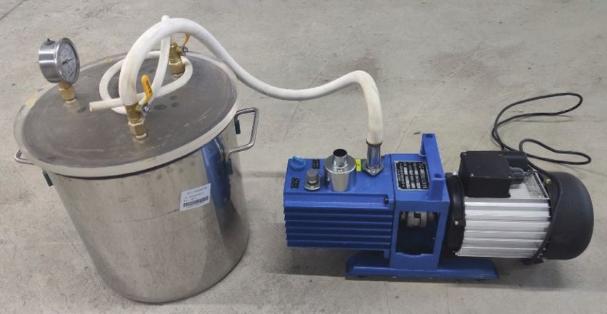
2                                                                                                               Shock and Vibration

                   Figure 1: Columnar jointed rock mass in the dam site area of the Baihetan hydropower station.

forward a modified cubic law by incorporating different def-           (0.2–0.8 MPa), and the change in permeability and the stress
initions of joint surface roughness [13–16]. However, the            sensitivity of the columnar jointed rock mass is analyzed at
variation of the joint surface roughness under stress is highly      different dip angles.
complex, resulting in a wide range of the joint gap width,
complicating the theoretical calculation of the seepage-stress
                                                                     2. Sample Preparation and Test Equipment
coupling of joints [17–19]. Therefore, it is feasible and effective
to conduct indoor seepage-stress coupling tests on rock              2.1. Sample Preparation. Ordinary Portland cement, river
samples to explore the seepage characteristics under stress. Liu     sand, and water with a mass ratio of 1 : 0.5 : 0.4 are used as
et al. investigated the nonlinear flow characteristics of a fluid at   the column materials of the similar material model to ensure
the fracture intersection using an indoor permeability test; they    that the physical and mechanical properties of the test
established a fracture network model to simulate the fluid flow        sample are similar to that of the natural rock [26]. An early-
state and analyze the influence of the equivalent hydraulic gap       strength water-reducing agent of 0.4% cement quality was
width and hydraulic gradient on the nonlinear seepage char-          added to ensure the workability and cohesiveness of the
acteristics [20]; Liu and Li analyzed the relationship between       mortar and improve the strength of the column in the initial
water permeability and sand particle size using a self-designed      setting. The bonding material between the pillars consisted
seepage circuit [21]; Xia et al. studied the nonlinear seepage       of a mix of ordinary white Portland cement with the same
characteristics of a single joint surface with different roughness    quality and water with a ratio of 1 : 0.4.
values using an indoor shear seepage test [22, 23]; Liu et al.           A regular hexagonal prism with a side length of 15 mm
performed conventional indoor triaxial seepage tests on frac-        and a height of 160 mm was created to ensure that the
tured sandstone and analyzed its permeability characteristics        column samples were similar to those of the naturally oc-
[24]; Chao carried out a conventional triaxial cyclic loading and    curring columnar jointed rock mass at the dam site of the
unloading seepage test on a similar material model of a co-          Baihetan hydropower station. A self-designed and manu-
lumnar jointed rock mass with inert gas as the measuring             factured cylinder mold (Figure 2(a)) was used to create the
medium to determine the relationship between permeability            sample columns. The mold consisted of several resin plates.
and confining pressure [25]. Few reports were published on the        The two sides of the mold were attached to long bolts, and
seepage characteristics of multijointed rock masses, especially      the middle was fastened with a clamp to ensure easy as-
columnar jointed rock masses.                                        sembly and demolding after the column had solidified.
     A natural columnar jointed rock mass has large columns.             First, lubricating oil was evenly applied to the surface of the
However, indoor tests are limited by the sample size, and the        mold. The cement mortar was then poured in layers, and the
grinding of the natural rock core does not reflect the actual         mold was continuously vibrated to minimize bubble generation
column structure. Therefore, the most effective and reliable          and mortar settlement in the column. The mold was then
method to analyze the permeability characteristics of a              placed in a constant-temperature box, and the mold was re-
columnar jointed rock mass in indoor tests is the use of             moved after 24 h. The demolded column (Figure 2(a)) was
similar material for the samples. Based on this, according to        placed in a standard constant-temperature and constant-hu-
the natural columnar joint rock mass size and the similarity         midity curing box (temperature 20 ± 1°C; humidity 95 ± 1.5%,
principle of the model test, this study uses ordinary Portland       Figure 2(b)) for 28 d. Subsequently, the columns were bonded
cement and river sand to fabricate hexagonal prism cylinders         together with the bonding material and were cured for 28 d in
to simulate a natural columnar joint rock mass and uses              the curing box. The bonded and cured material was cut and
white cement which has the same grade as cementation                 ground into 100 × 100 × 100 mm samples of the cubic co-
material to make the similar material model sample of                lumnar jointed rock mass with column inclination angles of 0°,
hexagonal prism columnar jointed rock mass. A true triaxial          15°, 30°, 45°, 60°, 75°, and 90°, as shown in Figure 3.
electrohydraulic servo seepage test machine is used to
conduct a seepage-stress coupling test using distilled water
as the measuring medium. The volume velocity of samples              2.2. Test Equipment. The test equipment was a true triaxial
with different dip angles is determined under the maximum             electrohydraulic servo test machine to determine the rock
principal stress σ1 and different water pressures σ s                 fracture seepage (Figure 4). The test machine had a closed-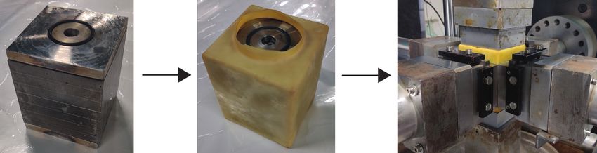
Shock and Vibration 3
(a) (b)
Figure 2: The mold for creating the column and the standard curing box.
Figure 3: Similar material samples of the columnar jointed rock masses with different dip angles.
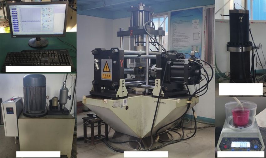
loop control system with an electrohydraulic servo valve to the required osmotic water pressure. The sample was
conduct the permeability test under triaxial loading. Three encased by O-rings placed on the upper and lower per-
directions were loaded independently to meet the require- meable plates and was wrapped in a latex membrane
ments of the rock permeability characteristics (including (Figure 5) to ensure that the seepage water could only pass
seepage deformation and seepage failure). through the cracks of the rock mass and did not flow in the
The seepage water weighing system is a crucial part of the transverse direction. The water seeped into the lower head
equipment and simulates the seepage velocity and water through the rock fracture and into the water container on
quantity of the rock fracture under different water pressures. the electronic balance through a water pipe. The electronic
The system consisted of a permeable water cylinder, servo balance was connected to a computer through a data in-
valve, pressure gauge and joint, high-precision electronic terface to collect data automatically. The relationship be-
balance, water collection container, water pipe, and other tween the rock sample’s triaxial stress and the seepage
components. The servo valve controls the pressure of the pressure, seepage velocity, and water quantity was
permeable water cylinder and ensures that the sample has determined.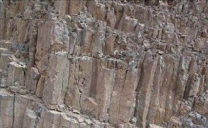
4                                                                                                                 Shock and Vibration

              Electronic control system

                                                                                                           Infiltration water
                                                                                                                  tank

                  Hydraulic source                                  Main engine                            Electronic balance

                           Figure 4: The true triaxial test system for determining the rock fracture seepage.

                   (a)                                      (b)                                           (c)
                                                    Figure 5: Sample installation.

2.3. Test Method and Test Scheme. Typical methods of the                      stress of σ 1 � σ 2 � σ 3 � 1 MPa was applied in the three
single-phase liquid seepage test in the laboratory include the                directions at a speed of 30 kN/min. σ 2 and σ 3
constant water head, variable water head, flow pump, and                       remained unchanged at 1 MPa, and σ 1 was loaded to
unstable pulse methods [27]. In this test, we used the constant               6 MPa with a step size of 1 MPa.
water head method. A water pressure difference was created at              (2) The loading method of the seepage water pressure:
both ends of the rock sample, and the flow velocity and the                    after each stage of stress loading was stable, the
fluid volume exiting the rock sample were determined.                          seepage water pressure σ s was applied at 0.2 MPa and
    Before the test, the model sample was placed into a                       was then increased to 0.8 MPa with a step size of
vacuum saturation device that used distilled water (Fig-                      0.1 MPa.
ure 6). The samples were wrapped with latex films and
loaded into the test machine. During the seepage test, the
fluid was assumed to be incompressible; the test was con-              3. Test Results and Analysis
ducted at a constant temperature of 23°C. During the test,
                                                                      3.1. The Analysis of the Seepage Characteristics with the
the maximum principal stress σ 1 was applied in the Z-axis
                                                                           Forchheimer Equation
direction, and the intermediate principal stress σ 2 and the
minimum principal stress σ 3 were applied in the transverse           3.1.1. The Relationship between Volume Velocity and Pressure
direction (Figure 7). The loading scheme was as follows:              Gradient. Figure 8 shows the relationship between the
    (1) The loading mode of the three-dimensional principal           volume velocity Q and the pressure gradient dP/dL of the
        stress: force-controlled loading was used. First, the         similar material samples with different inclination angles
        specimen was loaded to Fx � Fy � Fz � 1 kN. Then, the         under maximum principal stress loading.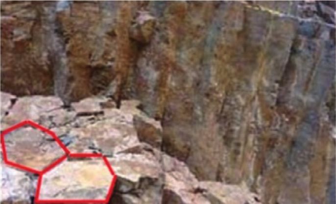
Shock and Vibration                                                                                                            5

                                             Figure 6: The vacuum saturation device.

                                    z                        σ1             Flow direction
                                             y

                                                 x

                                                                                             σ3

                                        σ2

                                Figure 7: The schematic diagram of stress and hydraulic loading.

    Significant differences are observed in the relationship        where ▽p � dP/dL is the ratio of the pressure difference P
between the volume velocity and the pressure gradient for         between the inlet and outlet and the length L of the sample;
the samples with different dip angles. At α � 0°–60°, the          Q is the overall volume velocity at the outlet; a and b are the
fitting curves show nonlinear characteristics, and the degree      model fitting coefficients, representing the specific gravity of
of nonlinearity is different. At the same stress, the flow rate     the water pressure drop caused by the linear term and
increases with an increase in the pressure gradient, indi-        nonlinear term in the seepage test, respectively. When b � 0,
cating an increase in the permeability of the sample. In          the Forchheimer function degenerates to Darcy’s law; μ is
contrast, at α � 75°–90°, linear Darcy flow characteristics are    the dynamic viscosity coefficient of the fluid; k is the intrinsic
observed.                                                         permeability of rock; A is the flow area of the rock; β is the
    For the nonlinear flow relationship in fractures and           nonlinear coefficient; ρ is the density of the fluid.
porous media, Forchheimer proposed a zero-intercept                   Table 1 lists the fitting coefficients a and b, the coeffi-
quadratic equation to describe the nonlinear flow process          cients of determination R2, the values of the intrinsic per-
from a macroscopic perspective [28, 29]:                          meability k, and the nonlinear coefficient β of the fractured
                                                                  rock obtained from equation (2). The R2 values of all test
                      −∇p � aQ + bQ2 ,                    (1)     conditions are greater than 0.98, indicating a good agree-
                                                                  ment between the experimental and simulated values. Thus,
                             μ                                    the Forchheimer equation is suitable to describe the rela-
                         a�    ,
                            kA                                    tionship between the volume velocity and pressure gradient
                            βρ                            (2)
                         b � 2,                                   of similar material samples of the columnar jointed rock
                            A                                     mass.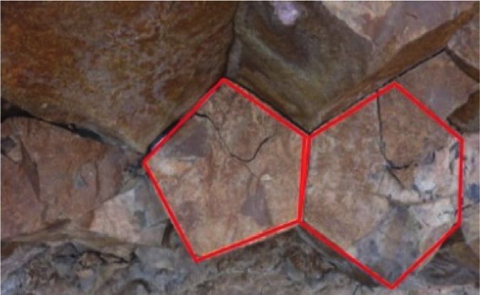
6                                                                                                                                                        Shock and Vibration

                    9                                                                                  9

                    8                                                                                  8

                    7                                                                                  7
    dP/dL (MPa/m)

                                                                                       dP/dL (MPa/m)
                    6                                                                                  6

                    5                                                                                  5

                    4                                                                                  4

                    3                                                                                  3

                    2                                                                                  2

                    1                                                                                  1
                             2          4       6         8       10       12     14                       0              4       8        12       16         20    24
                                                    Q (×10–8m3/s)                                                                     Q (×10–8m3/s)

                            σ1 =   1MPa                      Fit curve 1                                       σ1 =   1 MPa                      Fit curve 1
                            σ1 =   2MPa                      Fit curve 2                                       σ1 =   2 MPa                      Fit curve 2
                            σ1 =   3MPa                      Fit curve 3                                       σ1 =   3 MPa                      Fit curve 3
                            σ1 =   4MPa                      Fit curve 4                                       σ1 =   4 MPa                      Fit curve 4
                            σ1 =   5MPa                      Fit curve 5                                       σ1 =   5 MPa                      Fit curve 5
                            σ1 =   6MPa                      Fit curve 6                                       σ1 =   6 MPa                      Fit curve 6

                                                    (a)                                                                                 (b)
                    9                                                                                  9

                    8                                                                                  8

                    7                                                                                  7
    dP/dL (MPa/m)

                                                                                       dP/dL (MPa/m)

                    6                                                                                  6

                    5                                                                                  5

                    4                                                                                  4

                    3                                                                                  3

                    2                                                                                  2

                    1                                                                                  1
                        0           4       8        12       16           20     24                       0          4       8        12      16        20     24   28
                                                Q (×10–8m3/s)                                                                         Q (×10–8m3/s)
                            σ1 =   1MPa                      Fit curve 1                                       σ1 =   1 MPa                      Fit curve 1
                            σ1 =   2MPa                      Fit curve 2                                       σ1 =   2 MPa                      Fit curve 2
                            σ1 =   3MPa                      Fit curve 3                                       σ1 =   3 MPa                      Fit curve 3
                            σ1 =   4MPa                      Fit curve 4                                       σ1 =   4 MPa                      Fit curve 4
                            σ1 =   5MPa                      Fit curve 5                                       σ1 =   5 MPa                      Fit curve 5
                            σ1 =   6MPa                      Fit curve 6                                       σ1 =   6 MPa                      Fit curve 6

                                                    (c)                                                                                 (d)
                                                                            Figure 8: Continued.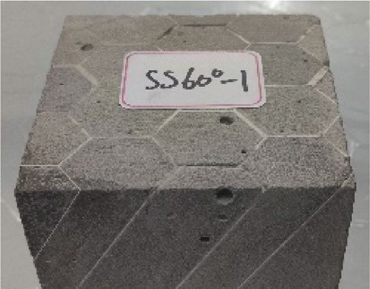
Shock and Vibration                                                                                                                                                                          7

                     9                                                                                                 9

                     8                                                                                                 8

                     7                                                                                                 7
     dP/dL (MPa/m)

                                                                                                       dP/dL (MPa/m)
                     6                                                                                                 6

                     5                                                                                                 5

                     4                                                                                                 4

                     3                                                                                                 3

                     2                                                                                                 2

                     1                                                                                                 1
                         0          2      4     6      8                      10         12    14                         0          2        4        6      8     10       12   14   16
                                               Q (×10–8m3/s)                                                                                             Q (×10–8m3/s)

                             σ1 =   1MPa                                Fit curve 1                                            σ1 =   1 MPa                          Fit curve 1
                             σ1 =   2MPa                                Fit curve 2                                            σ1 =   2 MPa                          Fit curve 2
                             σ1 =   3MPa                                Fit curve 3                                            σ1 =   3 MPa                          Fit curve 3
                             σ1 =   4MPa                                Fit curve 4                                            σ1 =   4 MPa                          Fit curve 4
                             σ1 =   5MPa                                Fit curve 5                                            σ1 =   5 MPa                          Fit curve 5
                             σ1 =   6MPa                                Fit curve 6                                            σ1 =   6 MPa                          Fit curve 6

                                                  (e)                                                                                                         (f )
                                                                    9

                                                                    8

                                                                    7
                                                    dP/dL (MPa/m)

                                                                    6

                                                                    5

                                                                    4

                                                                    3

                                                                    2

                                                                    1
                                                                        0          2      4    6      8     10                            12       14    16
                                                                                                Q (×10–8m3/s)
                                                                            σ1 =   1MPa                                    Fit curve 1
                                                                            σ1 =   2MPa                                    Fit curve 2
                                                                            σ1 =   3MPa                                    Fit curve 3
                                                                            σ1 =   4MPa                                    Fit curve 4
                                                                            σ1 =   5MPa                                    Fit curve 5
                                                                            σ1 =   6MPa                                    Fit curve 6

                                                                                                     (g)

Figure 8: The relationship between the volume velocity Q and the pressure gradient dP/dL for samples with different dip angles. (a) SS0°, (b)
SS15°, (c) SS30°, (d) SS45°, (e) SS60°, (f ) SS75°, and (g) SS90°.

    Table 1 indicates that the variation trend of the linear                                                     Figure 10 shows the relationship between the nonlinear
term coefficient a in the fitting equation of the samples with                                                  coefficient β and the maximum principal stress σ 1 for samples
different dip angles with an increase in the maximum                                                          with different dip angles. It can be seen that only the nonlinear
principal stress σ 1 is different. The trends are shown in                                                    coefficient β of the samples with dip angles of 75° and 90° is
Figure 9. It can be seen that at α � 0°–60°, the linear term                                                 positive when the stress has been initially loaded and the
coefficient a increases first and then decreases, at                                                            nonlinear coefficient β of other samples is negative. This
α � 75°–90°, and the linear term coefficient a increases                                                       phenomenon has also appeared in many scholars’ seepage tests;
monotonically.                                                                                               Liao et al. studied and discussed the possibility and causes of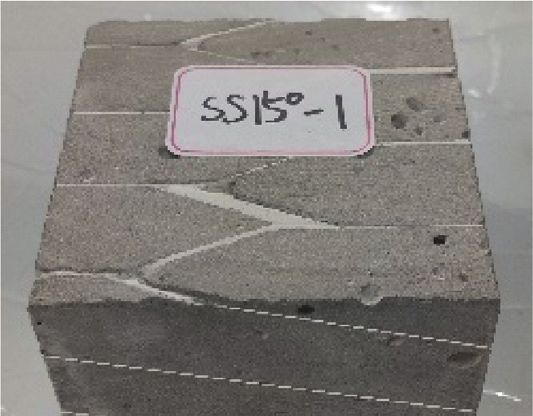
8 Shock and Vibration
Table 1: The fitting results of the nonlinear Forchheimer equation and the calculated values of k and β
Maximum Fitting Intrinsic
Sample Fitting coefficient a Coefficient of Nonlinear
principal stress coefficient b permeability k
number (Pa·s·m−4 × 10¹⁴) determination R2 coefficient β (m−1)
σ 1 (MPa) (Pa·s2·m−7 × 10²²) (m2)
1 8.078 E − 01 −1.361 E − 02 0.9993 1.579 E − 15 −6.765 E + 12
2 8.821 E − 01 −1.270 E − 02 0.9985 1.446 E − 15 −6.312 E + 12
3 9.157 E − 01 −1.049 E − 02 0.9991 1.393 E − 15 −5.214 E + 12
SS0°
4 9.852 E − 01 −1.543 E − 02 0.9991 1.294 E − 15 −7.669 E + 12
5 9.792 E − 01 −2.216 E − 02 0.9989 1.302 E − 15 −1.101 E + 13
6 8.043 E − 01 −1.372 E − 02 0.9976 1.585 E − 15 −6.819 E + 12
1 7.929 E − 01 −1.533 E − 02 0.9883 1.608 E − 15 −7.619 E + 12
2 9.268 E − 01 −2.202 E − 02 0.9877 1.376 E − 15 −1.094 E + 13
3 8.912 E − 01 −2.152 E − 02 0.9933 1.431 E − 15 −1.070 E + 13
SS15°
4 8.455 E − 01 −1.856 E − 02 0.9940 1.508 E − 15 −9.225 E + 12
5 7.246 E − 01 −1.476 E − 02 0.9946 1.760 E − 15 −7.336 E + 12
6 4.928 E − 01 −6.380 E − 03 0.9935 2.588 E − 15 −3.171 E + 12
1 8.718 E − 01 −1.875 E − 02 0.9982 1.463 E − 15 −9.319 E + 12
2 1.024 E + 00 −2.772 E − 02 0.9990 1.246 E − 15 −1.378 E + 13
3 1.113 E + 00 −3.456 E − 02 0.9960 1.146 E − 15 −1.718 E + 13
SS30°
4 1.027 E + 00 −3.233 E − 02 0.9963 1.242 E − 15 −1.607 E + 13
5 8.599 E − 01 −2.280 E − 02 0.9984 1.483 E − 15 −1.133 E + 13
6 6.127 E − 01 −1.117 E − 02 0.9987 2.081 E − 15 −5.552 E + 12
1 9.247 E − 01 −2.320 E − 02 0.9933 1.379 E − 15 −1.153 E + 13
2 9.551 E − 01 −2.243 E − 02 0.9952 1.335 E − 15 −1.115 E + 13
3 8.284 E − 01 −1.956 E − 02 0.9973 1.539 E − 15 −9.722 E + 12
SS45°
4 5.011 E − 01 −5.140 E − 03 0.9990 2.545 E − 15 −2.555 E + 12
5 4.406 E − 01 −3.710 E − 03 0.9996 2.894 E − 15 −1.844 E + 12
6 3.786 E − 01 −2.860 E − 03 0.9983 3.368 E − 15 −1.421 E + 12
1 8.4222 E − 01 −1.8600 E − 02 0.9965 1.514 E − 15 −9.245 E + 12
2 1.0840 E + 00 −2.3160 E − 02 0.9979 1.176 E − 15 −1.151 E + 13
3 1.1346 E + 00 −1.9720 E − 02 0.9961 1.124 E − 15 −9.801 E + 12
SS60°
4 1.0895 E + 00 −2.1190 E − 02 0.9963 1.170 E − 15 −1.053 E + 13
5 9.9456 E − 01 −2.4650 E − 02 0.9991 1.282 E − 15 −1.225 E + 13
6 7.7904 E − 01 −1.3570 E − 02 0.9992 1.637 E − 15 −6.745 E + 12
1 5.3832 E − 01 1.9100 E − 03 0.9867 2.369 E − 15 9.493 E + 11
2 6.5698 E − 01 2.1100 E − 03 0.9946 1.941 E − 15 1.049 E + 12
3 7.7073 E − 01 −1.0400 E − 03 0.9950 1.655 E − 15 −5.169 E + 11
SS75°
4 8.9612 E − 01 −6.2300 E − 03 0.9916 1.423 E − 15 −3.096 E + 12
5 1.0872 E + 00 −9.0500 E − 03 0.9963 1.173 E − 15 −4.498 E + 12
6 1.4753 E + 00 −2.6690 E − 02 0.9935 8.643 E − 16 −1.327 E + 13
1 5.4456 E − 01 1.6000 E − 03 0.9907 2.342 E − 15 7.952 E + 11
2 7.4407 E − 01 −6.7000 E − 03 0.9962 1.714 E − 15 −3.330 E + 12
3 8.9512 E − 01 −8.2300 E − 03 0.9975 1.425 E − 15 −4.091 E + 12
SS90°
4 9.2963 E − 01 −1.6400 E − 03 0.9975 1.372 E − 15 −8.151 E + 11
5 1.1876 E + 00 −2.8810 E − 02 0.9779 1.074 E − 15 −1.432 E + 13
6 1.3268 E + 00 −3.7120 E − 02 0.9802 9.611 E − 16 −1.845 E + 13
1.00 1.0 1.2 1.0
0.96 0.9 1.1 0.9
a (Pa·s·m–4 × 10¹⁴)
a (Pa·s·m–4 × 10¹⁴)
a (Pa·s·m–4 × 10¹⁴)
a (Pa·s·m–4 × 10¹⁴)
1.0 0.8
0.92 0.8
0.9 0.7
0.88 0.7 0.6
0.8
0.84 0.6 0.5
0.7
0.4
0.80 0.5 0.6
0.3
1 2 3 4 5 6 1 2 3 4 5 6 1 2 3 4 5 6 1 2 3 4 5 6
σ1 (ΜPa) σ1 (ΜPa) σ1 (ΜPa) σ1 (ΜPa)
(a) (b) (c) (d)
Figure 9: Continued.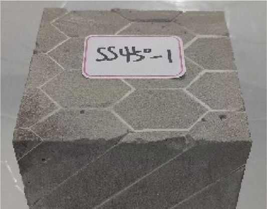
Shock and Vibration 9
1.15 1.6 1.4
1.10 1.4 1.2
a (Pa·s·m–4 × 10¹⁴)
a (Pa·s·m–4 × 10¹⁴)
a (Pa·s·m–4 × 10¹⁴)
1.05
1.00 1.2
1.0
0.95 1.0
0.90 0.8
0.8
0.85
0.6 0.6
0.80
0.75 0.4 0.4
1 2 3 4 5 6 1 2 3 4 5 6 1 2 3 4 5 6
σ1 (ΜPa) σ1 (ΜPa) σ1 (ΜPa)
(e) (f ) (g)
Figure 9: The relationship between the linear coefficient a and the stress for specimens with different dip angles. (a) SS0°, (b) SS15°, (c) SS30°,
(d) SS45°, (e) SS60°, (f ) SS75°, and (g) SS90°.
0.4
0.0
–0.4
β (1013m–1)
–0.8
–1.2
–1.6
–2.0
1 2 3 4 5 6
σ1 (ΜPa)
SS0° SS60°
SS15° SS90°
SS30° SS75°
SS45°
Figure 10: The relationship between the nonlinear coefficient β and the maximum principal stress σ 1.
negative values of β [27, 30–32]. In this test, the author believes obvious seepage anisotropy, and there are significant dif-
that the negative values of the nonlinear coefficients β reflect the ferences in the relationship between the natural permeability
test attributes of the similar material samples of the columnar k and the maximum principal stress σ 1 for samples with
jointed rock mass. There are two potential reasons: (1) A different dip angles. The relationship can be summarized
boundary layer exists on the surface of porous media. As the into two types: In the Type I curves (α � 0°–60°), the intrinsic
pressure gradient increases, the thickness of the boundary layer permeability decreases initially and then increases with an
decreases, and the cross-sectional area of the fluid and the increase in the maximum principal stress, showing a
permeability increase, resulting in a negative value of β. (2) U-shape. Define the stress when the permeability decreases
White cement was used as the filling medium between the and start to increase as the inflection point stress, and the
columns of the samples. As the pressure gradient increases, the inflection point stress is 5, 3, 4, 3, and 4 MPa for the samples
maximum stress the filling medium can bear is exceeded, with different dip angles. In the Type II curves (α � 75°–90°),
resulting in the formation of new fractures or the connection of the intrinsic permeability exhibits a monotonous decrease
the original fractures in the medium. The pore structure of the with an increase in the maximum principal stress, and the
medium is changed, increasing the porosity and permeability curve is L-shaped.
and resulting in a negative value of β. However, an in-depth According to the variation characteristics of the per-
investigation is required to reveal the underlying mechanism. meability-stress curve, try to fit the test data with one-
variable cubic polynomial function:
3.1.2. The Relationship between the Intrinsic Permeability k � a + bσ 1 + cσ 21 + dσ 31 , (3)
and the Maximum Principal Stress. Figure 11 shows the
relationship between the intrinsic permeability and the where k is the intrinsic permeability of the rock; σ 1 is the
maximum principal stress of the samples with different dip maximum principal stress; a, b, c, and d are the fitting
angles. The samples of the columnar jointed rock mass show parameters. The R2 values of all fitting curves are greater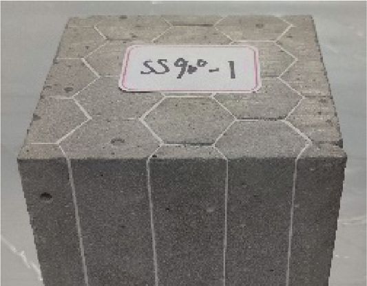
10 Shock and Vibration
1.65 2.8
1.60 2.6
1.55 2.4
y = 1.536 + 0.115x – 0.098x2 + 0.013x3 y = 1.67 – 0.028x – 0.076x2 + 0.018x3
1.50 R2 = 0.9593 2.2 R2 = 0.9842
k (×10–15m2)
k (×10–15m2)
1.45 2.0
1.40 1.8
1.35 1.6
1.30 1.4
1.25 1.2
1 2 3 4 5 6 1 2 3 4 5 6
σ1 (ΜPa) σ1 (ΜPa)
Calculated value Calculated value
Fit curve Fit curve
(a) (b)
2.2 3.6
3.3
2.0
3.0
y = 1.715 – 0.0261x – 0.005x2 + 0.01x3 y = 2.306 – 1.414x – 0.542x2 – 0.046x3
1.8 R2 = 0.9979 2.7 R2 = 0.9808
k (×10–15m2)
k (×10–15m2)
2.4
1.6
2.1
1.4 1.8
1.2 1.5
1.2
1.0
1 2 3 4 5 6 1 2 3 4 5 6
σ1 (ΜPa) σ1 (ΜPa)
Calculated value Calculated value
Fit curve Fit curve
(c) (d)
1.7 2.6
2.4
1.6
2.2
y = 1.979 – 0.579x + 0.104x2 – 0.003x3 2.0 y = 2.985 – 0.738x + 0.132x2 – 0.011x3
1.5
R2 = 0.9785 R2 = 0.9999
k (×10–15m2)
k (×10–15m2)
1.8
1.4
1.6
1.3 1.4
1.2
1.2
1.0
1.1 0.8
0.6
1 2 3 4 5 6 1 2 3 4 5 6
σ1 (ΜPa) σ1 (ΜPa)
Calculated value Calculated value
Fit curve Fit curve
(e) (f )
Figure 11: Continued.Shock and Vibration 11
2.6
2.4
2.2
y = 3.308 – 1.22x + 0.26x2 – 0.02x3
2.0 R2 = 0.9866
k (×10–15m2)
1.8
1.6
1.4
1.2
1.0
0.8
1 2 3 4 5 6
σ1 (ΜPa)
Calculated value
Fit curve
(g)
Figure 11: The relationship between the intrinsic permeability k and the maximum principal stress σ 1 for samples with different dip angles.
(a) SS0°, (b) SS15°, (c) SS30°, (d) SS45°, (e) SS60°, (f ) SS75°, and (g) SS90°.
than 0.96, indicating an excellent goodness-of-fit of the −∇p � λQm , (4)
cubic polynomial function describing the relationship
between the intrinsic permeability and the maximum where λ and m are empirical coefficients. When m � 1, the
principal stress of similar material samples of a columnar Izbash equation degenerates to the linear Darcy’s law. When
jointed rock mass. m � 1-2, equation (4) represents the nonlinear seepage
In addition, the values of the intrinsic permeability of the characteristics caused by a significant inertia effect. Values of
samples with different dip angles also show obvious an- m � 0-1 are often used to characterize nonlinear seepage in
isotropy. The initial permeability ks, the minimum perme- low-permeability rock media caused by a significant solid-
ability kmin, the maximum permeability kmax, and the final liquid interface effect.
permeability kf of the samples with different dip angles are The Izbash equation is used to fit the test data. The fitting
plotted in Figure 12. coefficients λ and m and the R2 values for different maxi-
The maximum decrease in the minimum permeability mum principal stress are listed in Table 2. The results show
relative to the samples’ initial permeability is 63.51% for the that the Izbash equation is suitable for characterizing the
specimen with a 75° dip angle, and the minimum decrease is nonlinear seepage characteristics of similar material samples
3.18% for the specimen with a 45° dip angle, representing a of the columnar jointed rock mass well. The R2 values are all
20-fold difference. The maximum permeability of the 45° greater than 0.98. The order of magnitude of the fitting
angle specimen increases by 144.25% compared with the coefficient λ is 1013–1014, and the range of the fitting coef-
initial permeability. The permeability of the 75° and 90° dip ficient m is between 0.68 and 1.02.
angle samples decreases monotonically, and the maximum The trends of the coefficients λ with the maximum
permeability is the same as the initial permeability. The principal stress σ 1 obtained from the Izbash equation for
maximum permeability of the 0° and 60° dip angle samples is samples with different dip angles are plotted in Figure 13. It
basically equal to the initial permeability. The final per- can be seen that the trend of the coefficients λ is basically
meability increases by 0.43%, 60.90%, 42.28%, 144.25%, and consistent with that of the linear coefficient a obtained from
8.11% for the 0°–60° dip angle samples, whereas decreases of the Forchheimer equation; there is a good corresponding
63.51% and 58.96% are observed for the 75° and 90° dip angle relationship between the two. In addition, there is also a
samples, respectively (compared with the initial perme- corresponding relationship between the two equations in
ability). The sensitivity of the permeability of the samples describing the nonlinear seepage characteristics of similar
with different dip angles to the maximum principal stress is material samples of columnar jointed rock mass; that is, the
α � 45° > α � 75° > α � 15° > α � 90° > α � 30° > α � 60° > α � 0°. fitting coefficient m < 1 of the Izbash equation corresponds
to the nonlinear coefficient β < 0 in the Forchheimer
equation.
3.2. Analysis of the Seepage Characteristics Using the Izbash Figure 14 shows the R2 values of the Forchheimer
Equation. The Izbash equation, which is a power function, equation and Izbash equations for fitting the test data. Both
has also been widely used to characterize the nonlinear the zero-intercept quadratic function (Forchheimer equa-
seepage characteristics of fluids [33]: tion) and the power function (Izbash equation) well describe12 Shock and Vibration
3.6
3.2
2.8
2.4
k (m2×10–12)
2.0
1.6
1.2
0.8
0 15 30 45 60 75 90
Dip angles (°)
ks kmax
kmin kf
Figure 12: The ks, kmin, kmax, and kf of samples with different dip angles.
Table 2: The fitting parameters of the Izabsh equation.
Sample number Maximum principal stress σ 1 (MPa) Fitting coefficient λ Fitting coefficient m Coefficient of determination R2
1 9.326 E + 13 0.85 0.9975
2 9.744 E + 13 0.89 0.9992
3 9.798 E + 13 0.92 0.9995
SS0°
4 1.072 E + 14 0.89 0.9995
5 1.140 E + 14 0.82 0.9984
6 9.529 E + 13 0.84 0.9993
1 9.895 E + 13 0.80 0.9892
2 1.142 E + 14 0.79 0.9898
3 1.139 E + 14 0.77 0.9914
SS15°
4 1.067 E + 14 0.78 0.9945
5 1.006 E + 14 0.75 0.9966
6 7.177 E + 13 0.77 0.9988
1 1.043 E + 14 0.81 0.9930
2 1.229 E + 14 0.78 0.9928
3 1.353 E + 14 0.76 0.9888
SS30°
4 1.395 E + 14 0.69 0.9833
5 1.266 E + 14 0.68 0.9847
6 9.560 E + 13 0.71 0.9921
1 1.140 E + 14 0.78 0.9864
2 1.117 E + 14 0.82 0.9900
3 1.100 E + 14 0.75 0.9908
SS45°
4 6.255 E + 13 0.85 0.9992
5 5.451 E + 13 0.87 0.9993
6 4.901 E + 13 0.86 0.9993
1 1.069 E + 14 0.78 0.9954
2 1.202 E + 14 0.86 0.9983
3 1.226 E + 14 0.89 0.9974
SS60°
4 1.207 E + 14 0.87 0.9983
5 1.188 E + 14 0.80 0.9989
6 9.357 E + 13 0.83 0.9989
1 5.369 E + 13 1.02 0.9863
2 6.519 E + 13 1.02 0.9944
3 7.757 E + 13 0.99 0.9950
SS75
4 9.339 E + 13 0.95 0.9919
5 1.100 E + 14 0.96 0.9959
6 1.496 E + 14 0.93 0.9928Shock and Vibration 13
Table 2: Continued.
Sample number Maximum principal stress σ 1 (MPa) Fitting coefficient λ Fitting coefficient m Coefficient of determination R2
1 5.618 E + 13 1.00 0.9903
2 8.247 E + 13 0.91 0.9978
3 9.540 E + 13 0.93 0.9982
SS90°
4 9.515 E + 13 0.98 0.9977
5 1.364 E + 14 0.83 0.9857
6 1.497 E + 14 0.83 0.9877
1.15 1.2 1.5 1.2
1.1 1.4 1.1
1.10
1.0
1.3
λ (×1014)
λ (×1014)
1.0
λ (×1014)
λ (×1014)
1.05 0.9
0.9 1.2 0.8
1.00
1.1 0.7
0.8
0.95 0.6
1.0
0.7 0.5
0.90 0.9 0.4
1 2 3 4 5 6 1 2 3 4 5 6 1 2 3 4 5 6 1 2 3 4 5 6
σ1 (ΜPa) σ1 (ΜPa) σ1 (ΜPa) σ1 (ΜPa)
(a) (b) (c) (d)
1.25 1.6 1.6
1.20 1.4 1.4
1.15
1.2 1.2
λ (×1014)
λ (×1014)
λ (×1014)
1.10
1.0 1.0
1.05
0.8 0.8
1.00
0.95 0.6 0.6
0.90 0.4 0.4
1 2 3 4 5 6 1 2 3 4 5 6 1 2 3 4 5 6
σ1 (ΜPa) σ1 (ΜPa) σ1 (ΜPa)
(e) (f ) (g)
Figure 13: The relationship between the fitting coefficient λ of the Izbash equation and the stress for samples with different dip angles. (a)
SS0°, (b) SS15°, (c) SS30°, (d) SS45°, (e) SS60°, (f ) SS75°, and (g) SS90°.
1.005
1.000
0.995
R2 0.990
0.985
0.980
0.975
0 4 8 12 16 20 24 28 32 36 40 44
Data set
Forchheimer
Izbash
Figure 14: The R2 values of the Forchheimer and Izbash equations under all working conditions.14 Shock and Vibration
the nonlinear flow of the similar material samples of the Data Availability
columnar jointed rock mass, and the difference between
them is not significant. However, the Forchheimer equation All the data in this paper are obtained by experiments and
has a clear theoretical basis and can be simplified by the have been presented in this manuscript.
Navier-Stokes equation if the flow channel does not change
significantly. In contrast, the Izbash equation is purely Conflicts of Interest
empirical without clear physical meaning.
The authors declare no conflicts of interest.
4. Conclusions Acknowledgments
In this paper, the seepage characteristics of a columnar This research was funded by the National Natural Science
jointed rock mass under maximum principal stress were Foundation of China (Grants nos. 41831278, 51579081, and
investigated using similar material samples with different 51709184), the Postgraduate Research and Practice Innovation
dip angles and conducting seepage-stress coupling tests. The Program of Jiangsu Province (Grant no. 2018B661X14), the
main conclusions are as follows: Natural Science Foundation of Jiangsu Province (Grant no.
(1) Under maximum principal stress, the seepage BK20161508), and the Central Public-Interest Scientific Insti-
characteristics of the similar material samples of the tution Basal Research Fund (Grant no. Y118008), Nanjing
columnar jointed rock mass showed anisotropic Hydraulic Research Institute, Nanjing, China.
characteristics. The permeability of samples with
different dip angles has different sensitivity to stress, References
and the law and degree of variation with stress are
[1] W. Y. Xu, W. T. Zheng, and A. C. Shi, “Classification and
also different.
quality assessment of irregular columnar jointed basaltic rock
(2) The relationship between the volume velocity Q and mass for hydraulic engineering,” Journal. Hydraulic Engi-
the pressure gradient dP/dL of the samples with neering, vol. 3, pp. 262–270, 2011.
different dip angles showed nonlinear seepage [2] C. F. Ke and S. L. Yu, “Characteristics of excavation-induced
characteristics. The Forchheimer equation accurately relaxation of columnar jointed basalt in the left bank dam
described the relationship, and the R2 values were foundation of Baihetan Hydropower station,” Journal of
greater than 0.98. In most cases, the nonlinear co- Yangtze River Scientific Research Institute, vol. 6, pp. 128–131,
2017.
efficient β was negative, which was attributed to the
[3] K. Kim and M. L. Cramer, “Rock mass deformation properties
test properties and the unique geological structure of of closely jointed basalt,” Rock Mechanics, vol. 1, pp. 210–230,
the similar material samples. 1982.
(3) The relationship between the intrinsic permeability k [4] M. L. Cramer and M. T. Black, “Design and construction of a
and the maximum principal stress σ 1 of the samples block test in closely jointed rock,” International Journal of
with different dip angles was categorized into two Rock Mechanics and Mining Sciences, vol. 2, p. 51, 1984.
types. In the Type I curves, the permeability initially [5] W.-M. Xiao, R.-G. Deng, Z.-B. Zhong, X.-M. Fu, and
decreased and then increased with an increase in the C.-Y. Wang, “Experimental study on the mechanical prop-
erties of simulated columnar jointed rock masses,” Journal of
maximum principal stress, showing a U-shape. In
Geophysics and Engineering, vol. 12, no. 1, pp. 80–89, 2015.
the Type II curves, the permeability showed a mo- [6] W. Lu, Z. Zhu, X. Que, C. Zhang, and Y. He, “Anisotropic
notonous decrease with an increase in the maximum constitutive model of intermittent columnar jointed rock
principal stress, and the curve was L-shaped. The masses based on the cosserat theory,” Symmetry, vol. 12, no. 5,
relationship can be well described by the cubic p. 823, 2020.
polynomial function equation k � a + bσ 1 + [7] M. Bai and D. Elsworth, Coupled Processes in Subsurface
cσ 21 + dσ 31 , and the R2 values are greater than 0.96. Deformation, Flow, and Transport, American Society of Civil
Engineers, Reston, VA, USA, 2000.
(4) The final permeability of the samples with 0°–60° dip
[8] Y. T. Zhang, Rock Hydraulics and Engineering, China Water &
angles increased compared with the initial perme- Power Press, Beijing, China, 2005.
ability, and that of the 45° dip angle sample increased [9] Y. Q. Wu and Z. Y. Zhang, Introduction to Rock Mass Hy-
by 144.25%, exhibiting the highest sensitivity to draulics, Southwest Jiaotong University Press, Shanghai,
stress. In contrast, the decreases were 63.51% and China, 1995.
58.96% for the 75° and 90° dip angle samples, [10] G. C. Zhang, Z. J. Wen, S. J. Liang et al., “Ground response of a
respectively. gob-side entry in a longwall panel extracting 17 m-thick coal
(5) The Izbash equation, a power function, also accu- seam: a case study,” Rock Mechanics and Rock Engineering,
vol. 53, no. 2, pp. 497–516, 2020.
rately described the nonlinear flow characteristics of
[11] C. A. Louis, Study of Groundwater Flow in Jointed Rock and its
the similar material samples of the columnar jointed Influence on the Stability of Rock Masses, pp. 91–98, Rock
rock mass, with R2 values greater than 0.98. The Mechanics Research Reports Imperial College, London, UK,
fitting coefficients λ and m were in good corre- 1969.
spondence with the linear coefficient a and the [12] E. S. Romm, Flow Characteristics of Fractured Rocks, Nedra
nonlinear coefficient β in the Forchheimer equation. Publishers, Moscow, Russia, 1966.Shock and Vibration 15
[13] J. B. Walsh, “Effect of pore pressure and confining pressure on Journal of Theoretical and Applied Mechanics, vol. 6,
fracture permeability,” International Journal of Rock Me- pp. 660–667, 2003.
chanics and Mining Sciences & Geomechanics Abstracts, [31] T. Z. Li, L. Ma, and L. Y. Zhang, “Discussion about positive or
vol. 18, no. 5, pp. 429–435, 1981. negative sign of permeability indexes in non-Darcy flow of
[14] C. E. Neuzil and J. V. Tracy, “Flow through fractures,” Water mudstone,” Journal of Mining & Safety Engineering, vol. 4,
Resources Research, vol. 17, no. 1, pp. 191–199, 1981. pp. 481–485, 2007.
[15] Y. W. Tsang and C. F. Tsang, “Channel model of flow through [32] W. L. Li, J. Q. Zhou, C. L. He, Y. F. Chen, and C. B. Zhou,
fractured media,” Water Resources Research, vol. 23, no. 3, “Nonlinear flow characteristics of broken granite subjected to
pp. 467–479, 1987. confining pressures,” Rock and Soil Mechanics, vol. S1,
[16] C. B. Zhou and W. L. Xiong, “A generalized cubic law for pp. 140–150, 2017.
percolation in rock joints,” Rock and Soil Mechanics, vol. 4, [33] S. V. O. Izbash, Filtracii V Kropnozernstom Materiale. USSR,
pp. 1–7, 1996. Russian, Leningrad, Russia, 1931.
[17] G. C. Zhang, Y. L. Tan, and S. J. Liang, “Numerical estimation
of suitable gob-side filling wall width in a highly gassy
longwall mining panel,” International Journal of Geo-
mechanics, vol. 8, pp. 04018091.1–04018091.15, 2018.
[18] T. Lu, R. Xu, B. Zhou, Y. Wang, F. Zhang, and P. Jiang,
“Improved method for measuring the permeability of
nanoporous material and its application to shale matrix with
ultra-low permeability,” Materials, vol. 12, no. 9,
pp. 1567–1588, 2019.
[19] C. Zhang, Z. Zhu, S. Zhu et al., “Nonlinear creep damage
constitutive model of concrete based on fractional calculus
theory,” Materials, vol. 12, no. 9, pp. 1505–1518, 2019.
[20] R. Liu, B. Li, and Y. Jiang, “Critical hydraulic gradient for
nonlinear flow through rock fracture networks: the roles of
aperture, surface roughness, and number of intersections,”
Advances in Water Resources, vol. 88, pp. 53–65, 2016.
[21] Y. Liu and S. Li, “Influence of particle size on non-Darcy
seepage of water and sediment in fractured rock,” Spring-
erplus, vol. 1, pp. 2099–2113, 2016.
[22] C. C. Xia, X. Qian, P. Lin, W. M. Xiao, and G. Yang, “Ex-
perimental investigation of nonlinear flow characteristics of
real rock joints under different contact conditions,” Journal of
Hydraulic Engineering, vol. 3, pp. 04016090.1–04016090.14,
2016.
[23] Q. Yin, G. Ma, H. Jing et al., “Hydraulic properties of 3D
rough-walled fractures during shearing: an experimental
study,” Journal of Hydrology, vol. 555, pp. 169–184, 2017.
[24] X. Liu, Z. Zhu, and A. Liu, “Permeability characteristic and
failure behavior of filled cracked rock in the triaxial seepage
experiment,” Advances in Civil Engineering, vol. 2019, pp. 1–12,
2019.
[25] Z. M. Chao, H. L. Wang, W. Y. Xu, H. Ji, and K. Zhao,
“Permeability and porosity of columnar jointed rock under
cyclic loading and unloading,” Chinese Journal of Rock Me-
chanics and Engineering, vol. 1, pp. 124–141, 2017.
[26] Y. Kong, Study on deformation failure mechanism and seepage
stress coupling characteristics of columnar jointed rock mass,
Ph.D. thesis, Hohai University, Nanjing, China, 2020.
[27] Y. Z. Huang, Mechanism of non-linear seepage flow in low
permeability rock and its variable permeability numerical
solution, Ph.D. thesis, Tsinghua University, Beijing, China,
2006.
[28] P. H. Forchheimer, “Wasserbewegung durch boden,” Zeit.
Ver. Deutsch. Ing, vol. 45, pp. 1782–1788, 1901.
[29] J.-Q. Zhou, S.-H. Hu, S. Fang, Y.-F. Chen, and C.-B. Zhou,
“Nonlinear flow behavior at low Reynolds numbers through
rough-walled fractures subjected to normal compressive
loading,” International Journal of Rock Mechanics and Mining
Sciences, vol. 80, pp. 202–218, 2015.
[30] X. X. Liao, Z. Q. Chen, X. B. Mao, and R. H. Chen, “The
bifurcation of non-Darcy flow in post-failure rock,” ChineseYou can also read