Five Methods of Exoplanet Detection - Journal of Physics: Conference Series - IOPscience

Journal of Physics: Conference Series

PAPER • OPEN ACCESS

Five Methods of Exoplanet Detection
To cite this article: Ziqi Dai et al 2021 J. Phys.: Conf. Ser. 2012 012135

View the article online for updates and enhancements.

 This content was downloaded from IP address 46.4.80.155 on 15/09/2021 at 20:31

ICMMAP 2021 IOP Publishing
Journal of Physics: Conference Series 2012 (2021) 012135 doi:10.1088/1742-6596/2012/1/012135

Five Methods of Exoplanet Detection

 Ziqi Dai1, a, *, †, Dong Ni2, b, *, †, Lizhuang Pan3, c, *, †, Yiheng Zhu4, d, *, †
 1
 Jiangsu Tianyi High School, Wuxi, Jiangsu, 214000, China
 2
 HolyCross High School, Waterbury, Connecticut, 06418, United States
 3
 University of Colorado Boulder, Boulder, Colorado, 80309, United States
 4
 Wuxi No.1 High School, Wuxi, Jiangsu, 214000, China
 *
 Corresponding author e-mail: adaiziqi2004@outlook.com, bni.dong@holycrosshs-
 ct.com, clipa3738@colorado.edu, dian.yeng@icloud.com
 †
 These authors contributed equally.

 Abstract. The study of exoplanetary systems can help us understand the formation and evolution
 of the solar system itself and search for terrestrial planets in the habitable and extrasolar lives in
 exoplanetary systems. Exoplanets have become an important area of astrophysics in the last two
 decades. This paper reviews five different methods to detect exoplanets, including direct imaging,
 astrometry, radial velocity, transit event observation, and microlensing. These approaches could
 expand the sample size of exoplanets and further our understanding of the types, formation and
 evolution of exoplanets.

1. Introduction
Whether there are other Earth-like planets with life in the universe or whether there are exoplanets has
always been attracting the attention of researchers. It was not until 1995 that a paper published by Mayor
& Queloz in Nature changed people’s imagination of exoplanets, and researchers discovered a planet
with a minimum mass of 51% of the mass of Jupiter through long-term measurement of the radial
velocity of the sun-like star 51 Peg [1]. This discovery has started the prelude to the study of extrasolar
planets. In addition, as early as 1992, Wolszczan and Frail detected three planetary companion objects
orbiting the pulsar PSRB1257+12 [2]. However, due to the extremely strong magnetic field of the host
star, the surrounding planets are not suitable for reproducing life like the Earth. On the other hand, these
planets may be formed by the remains of the precursor stars that formed pulsars after the explosion,
rather than formed together with the precursor stars or after the precursor stars entered the main sequence
stage.
 After just a few decades, by March 21, 2021, 4699 exoplanets have been confirmed
(www.exoplanet.eu). Before 2009, the launch of the Kepler Space Telescope by the National
Aeronautics and Space Administration (NASA), the exoplanets were detected dominantly by the radial
velocity method, while after the release of the data from the Kepler space survey, the detection was
immediately dominated by the predation event observation method. All this is attributed to the superb
design of the Kepler Space Telescope, which has unprecedented pointing accuracy and photometric
accuracy at the scale of one millionth (ppm), thus ensuring the ability to detect terrestrial planets and
even smaller exoplanets. The Transiting Exoplanet Survey Satellite (TESS), which was launched aboard
a SpaceX Falcon 9 rocket on April 18, 2018, is the next step in searching for planets beyond our solar

 Content from this work may be used under the terms of the Creative Commons Attribution 3.0 licence. Any further distribution
 of this work must maintain attribution to the author(s) and the title of the work, journal citation and DOI.
Published under licence by IOP Publishing Ltd 1

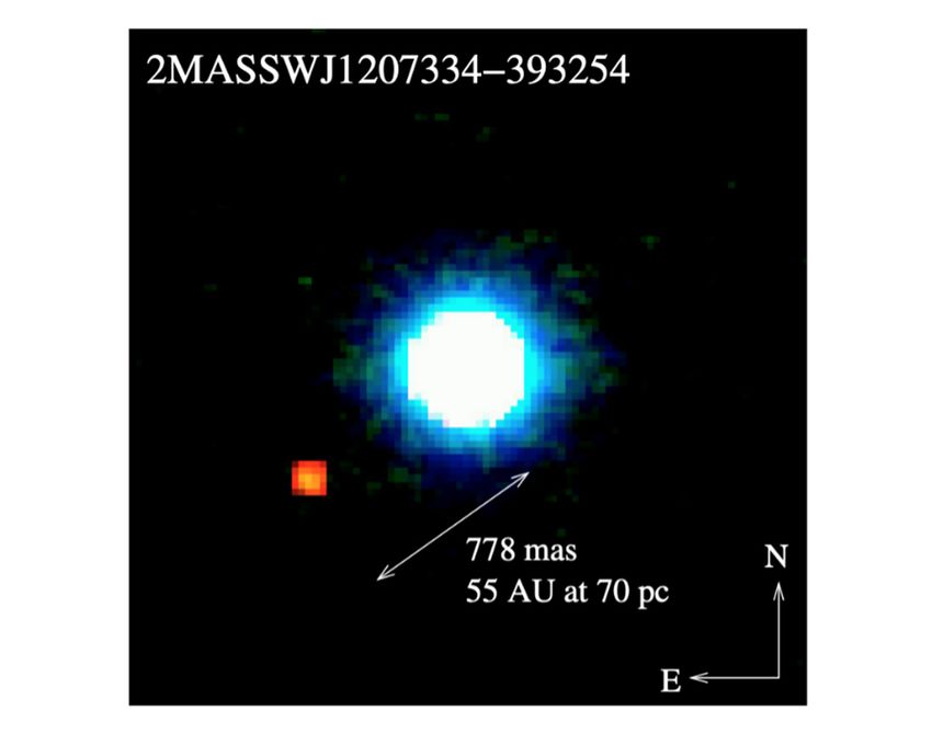
ICMMAP 2021 IOP Publishing
Journal of Physics: Conference Series 2012 (2021) 012135 doi:10.1088/1742-6596/2012/1/012135

system, including the search for bodies that could support life. TESS aims to survey 200,000 of the
brightest stars near the sun to search for exoplanets by catching transits. At present, the extrasolar planet
detection technology covers not only the pulsar timing method and the radial velocity method that
detected the first exoplanets. It also covers the newly developed gravitational microlensing method,
transit event observation method, direct imaging method, and astrometry. These detection methods have
been widely used and improved in the ongoing ground-based and space-based exoplanet search projects
[3, 4]. In the following sections, we will describe each of these detection methods.

2. Direct Imaging Method
Exoplanet imaging usually means the point source image formed by the light of the host star reflected
in target source detection and is different from the resolution of the planet surface. When the radius of
the planet is large and the orbit radius around the host star is relatively large, the method of adaptive
optics and coronagraph direct imaging can be used to detect exoplanets. This is because, in this case,
the planet is bright enough to be detected, and the host star is far enough away from the planet for the
telescope to be able to distinguish it. In 2004, Chauvin et al. detected the exoplanet 2M1207b discovered
with the direct imaging method for the first time by using Chile's Paranal Observatory's Very Large
Telescope [5] (as shown in Figure 1). The mass and effectiveness and temperature are predicted as 5 ±
2 Mjup and 1250 ± 200 K. The brightness ratio between the planet and the host star depends on the
planet's size, the distance between the planet and the star, and the scattering characteristics of the planet's
surface. The brightness ratio between the planet and the host star at wavelength λ is [6]:
 fα (α,λ) Rp 2 （1）
 =p(λ) g(α)，
 f* (λ) α

where p(λ) is the geometric albedo, and g(α) is the phase function of the planet. The brightness ratio
between the planet and the host star is usually very small. For example, the brightness ratio between a
Jupiter-like planet and a sun-like star in a system with a distance of 11 pc and the angular distance of
0.52 arcsec from us is 10-8~10−9.

 Figure 1. The CCD frame of 2M1207b [5].

 2

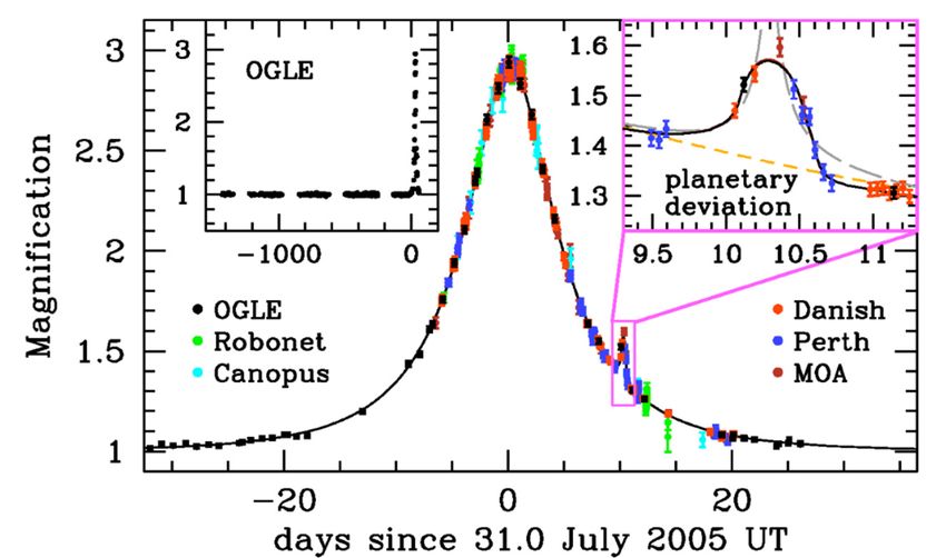
ICMMAP 2021 IOP Publishing
Journal of Physics: Conference Series 2012 (2021) 012135 doi:10.1088/1742-6596/2012/1/012135

3.Astrometry Method
Gatewood expounded the idea of using astrometry to detect exoplanets [7]. As shown in Figure 2, until
2010, Muterspaugh et al. detected the exoplanet HD 176051b by astrometry for the first time [8].
Astrometry is to detect planets by directly detecting the position of the host star perturbed by the planet’s
gravitational force, so it can get the planet’s mass and orbital inclination [3]. The host star's orbit around
the center of mass of the planet and the star is projected onto the sky plane usually as an ellipse, and the
angular semi-major axis α of the ellipse is [6]:
 -1
 Mp Mp a d （2）
 α= a= arcsec，
 M* +Mp M* +Mp 1AU 1pc
where a is the semi-major axis of the planetary orbit, and d is the distance from the system to the observer.
The observable α is directly proportional to the mass of the planet and the semi-major axis of the orbit
and inversely proportional to the distance. From the above derivation, the observation of at least one
complete orbit is the key to the astrometric detection of exoplanets. More periodic observations can
improve the confidence of the method.

 Figure 2. The perturbation of the position of primary star by the exoplanet HD 176051b detected
 by astrometry for the first time [8].

4.Radial Velocity Method
So far, about a fifth of all known exoplanets has been discovered by the radial velocity method. For
planets with large masses and short periods, the radial velocity method is applicable. The essence of this
method is to detect exoplanets by measuring the periodic variation of the star relative to the center of
mass of the system. Figure 3 shows the radial velocity of the first solar-like exoplanet, 51 Peg [1].
Currently, the detection accuracy of the radial velocity method has exceeded 1 m/s, which can detect
short period terrestrial planets surrounding M-type dwarfs [9,10].
 In general, the orbits of the planets are assumed to be elliptical. The reasons for this assumption can
be based on the orbits of the planets in our solar system and the current study of other exoplanets. One
can use the center of mass of the star and the planet as the origin and the long axis of the planet's orbit
as the x-axis to establish the Cartesian coordinate system [6]. As shown in Figure 4, the position of the
planet is

 3

ICMMAP 2021 IOP Publishing
Journal of Physics: Conference Series 2012 (2021) 012135 doi:10.1088/1742-6596/2012/1/012135

 x = r cosν (3)

 y = r sinν , (4)

 z=0 , (5)

where is the distance from the planet to the center of mass. Based on the elliptic equation, can be
replaced by:

 1-e2 (6)
 r=a ,
 1+e cosυ

where represents the angle between the line between the planet and the star and the line between the
orbit pericentre and the center of mass, a is the semi-major axis of the planet’s orbit while e is the
eccentricity of the planet’s orbit. In addition, can be transformed into a function of time t with the
following equation:
 v 1+e E (7)
 tan = tan ,
 2 1-e 2

 M=E-e sinE , (8)
 2π (9)
 M= (t-tp ) ,
 P

 as a reference time, which indicates the time when the planet passes through the pericentre while 
is the orbital period of the planet.

 Figure 3. Curve of the radial velocity of 51 Peg measured by Mayor & Queloz [1].

 4

ICMMAP 2021 IOP Publishing
Journal of Physics: Conference Series 2012 (2021) 012135 doi:10.1088/1742-6596/2012/1/012135

 Figure 4 Schematic diagram of tracks of exoplanet and its corresponding parameters[11].

 In actual observations, the orbit of a planet one observes is a projection of the planet's orbit in the
celestial coordinate system. As shown in Figure 5, the line of sight of the observer is parallel to the z-
axis, and a Cartesian coordinate system is built with the center of mass as the origin, so the position of
the planet can be characterized as [6]:
 x‾ =r cos Ω cos v+ω - sin Ω sin v+ω cos i , (10)

 y‾ =r sin Ω cos v+ω + cos Ω sin v+ω cos i , (11)

 z‾=rsin(v+ω)sin i . (12)
 Take the derivative of time over to get the radial velocity of the planet, multiplied by the mass
ratio of the planet to the star that can get the radial velocity Vr of the star around the barycentre
 ∗
of the system is obtained:
 Vr =V0 +K cos ν+ω +e cos ω ， (13)

 2πG 1/3 Mp sini (14)
 K= 2/3 ，
 P M* +Mp 1-e2

where is the radial velocity of the barycentre, G is a constant of the gravitation. Because ≪
 ∗ , approximating the expression to the radial velocity, the minimum mass of a planet can be expressed
(in terms of the mass of the earth):

 5

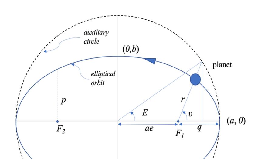
ICMMAP 2021 IOP Publishing
Journal of Physics: Conference Series 2012 (2021) 012135 doi:10.1088/1742-6596/2012/1/012135

 2/3 1/3 (15)
 Mp sini M* P
 =11.19 m/s×K 1-e2 .
 M⊕ M⊙ 1yr

 Figure 5. Schematic diagram of planetary orbits with its parameters [11].

5. Transit event observation method
More than 3,000 exoplanets have been discovered by detecting signals from periodic planetary transits.
In this method, the observer, the planet, and the host star are close to collinear. When the planet is
between the observer and the host star, the planet will pass through the front of the host star, causing
part of the star's light to be blocked by the planet. This blocking will be shown in the photometric
measurement of the star. This is called a transit event. Figure 6 shows the eclipse light curve of the first
exoplanet observed by Charbonneau et al. using the eclipse event observation method [12]. By analyzing
the solar eclipse curve of the planet, not only the radius of the planet but also the inclination of the plane
of the orbit and the long half axis of the orbit can be obtained.
 In the above part, we obtained the line of sight velocity dependency on the orbit of the parameters
and the planet’s mass. Based on the above relation, we can easily obtain the partial relation of the eclipse
light curves. The plane formed by- xoy is the sky plane, and the distance from the trajectory of the planet
in this plane to the origin multiply by a factor of 1+Mp/M* is the distance rsky from the center of the
planetary disk to the center of the stellar disk [6]:
 Mp Mp (16)
 rsky = 1+ x‾ 2 +y‾ 2 = 1+ r 1-sin2 (v+ω)sin2 i ，
 M* M*

 If the planet transit event occur, the required rsky minimum value rsky min satisfies rsky min < Rp+R*.
Taking rsky derivative v and making it zero(0), then we can obtain rsky, and take rsky satisfactory needed
condition:
 2
 a2 1-e2 (17)
 (1+e cosv)sin(2γ+2ω)sin2 i-2e sinf 1-sin2 isin2 (v+ω) =0 .
 (1+e cosv)3

 6

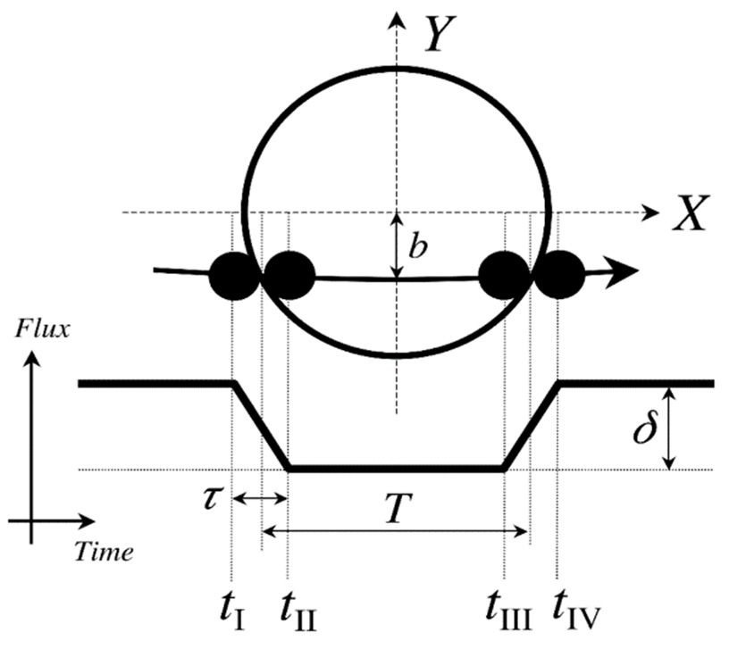
ICMMAP 2021 IOP Publishing
Journal of Physics: Conference Series 2012 (2021) 012135 doi:10.1088/1742-6596/2012/1/012135

 Figure 6. Charbonneau et al. first observation of HD209458b [12].
 Kipping obtained rsky min corresponding true anomaly vmin as [6,13]:
 n
 π (18)
 vmin = -ω+ ηκ ，
 2 k=1

 e cosω 1 (19)
 η1 = cos2 i ，
 1+e sinω

 e cosω 1 2 (20)
 η2 = cos2 i ，
 1+e sinω 1+e sinω

 e cosω -6 1+e sinω +e2 cos2 ω(-1+2e sinω) 3 (21)
 η3 =-( )[ 3 ](cos2 i) .
 1+e sinω 6(1+e sinω)
 For the transit eclipse system, the planet’s orbital plane is straightly close to the line direction, thus
the last term of sum in Equation 18 is quite a small quantity. In the actual transit eclipse curve dealing
process, we can ignore it. Take the approximate result of Equation 18 to Equation 16 to obtain rsky min:
 Mp a(1-e2 ) (22)
 rsky,min =(1+ ) cosi ，
 M* 1+e sinω

 In the field of exoplanet research, the collision parameter b is usually used to characterize the planet’s
eclipse trajectory distance and the center of the star’s disk as shown in Figure 7, and b is defined as:
 rsky,min
 b= ， (23)
 R*

 Due to the duration of the eclipse T14 ≤ p, therefore we can reasonably assume that the planet is
moving at a customary speed when the eclipse occurs, so the distance between the planet and star
remains unchanged. The distance between the planet and star ̅ is well approximated:
 1-e2 (24)
 r̅=a .
 1+e sinω

 Then, combined with Kepler’s Second law,

 7

ICMMAP 2021 IOP Publishing
Journal of Physics: Conference Series 2012 (2021) 012135 doi:10.1088/1742-6596/2012/1/012135

 Figure 7. The illustration of the eclipse light curve with its parameters [14].

 1 2 dv πa2 1-e2 (25)
 r̅ = ，
 2 dt P

 For Equation 25, the light becomes extremely small (corresponds to rsky min) t = Tmin integral to the
fourth touch of the planets and stars t = T4. One can obtain:

 ， (26)

 2πα (27)
 v4 -vmin = T4 -Tmin .
 P

 Among them, v4 shows the true apse angle of the planet at the fourth contact of the planet and the
star. The fourth contact and the time the light becomes extremely small, the difference is exactly half of
the duration T14. This time, the distance between the planet and astrolabe is Rp+R*. Therefore, the
following relationship exists,
 Mp α 1-e2 πα (28)
 Rp +R* = 1+ πα 1-cos2 T14 sin2 i .
 M* 1+e sin ω- T14 P
 P

 For a system composed of a Jupiter-like planet and a sun-like star, it is approximately 0.001. For a
system composed of a red short star and a Jupiter-like planet, Mp/M* is approximately 0.01. So in the
later calculations, Mp/M* will take two for approximation, then the physical parameters and model
parameters have the following relationship [6]:
 Planet to star radius ratio
 Rp (29)
 =√∆F ，
 R*

 The inclination of the planet’s orbit

 b2 - 1+√∆F
 2 (30)
 sini= .
 2
 b2 cos2 πα T - 1+√∆F
 P 14

 The semi major axis of the planet’s orbit in units of the star radius

 8

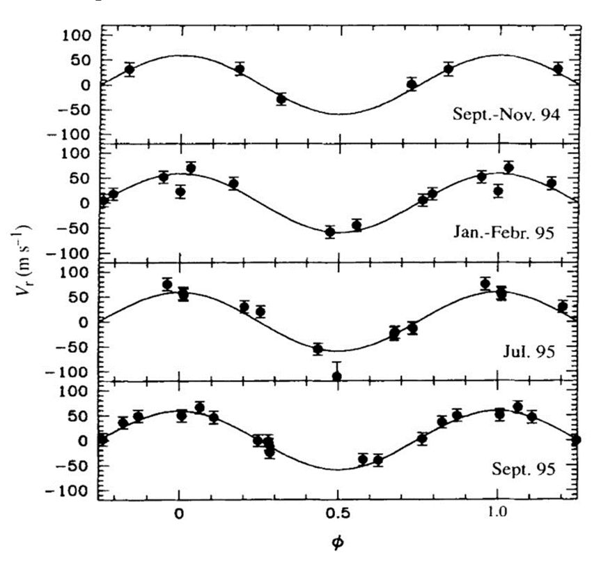
ICMMAP 2021 IOP Publishing
Journal of Physics: Conference Series 2012 (2021) 012135 doi:10.1088/1742-6596/2012/1/012135

 2
 1+√∆F -b2 cos2 πα T
 (31)
 a 1+e sinω P 14
 = .
 R* 1-e2
 sin2 πα T
 P 14

 The average density of stars can be derived as,
 2
 3π a 3 3π 1+e sinω 3 1+√∆F -b2 cos2 πa T
 P 14
 (32)
 p* = = .
 2
 GP R* GP 2
 1-e2 sin2 πa T
 P 14

6. Gravity Microlensing Effect
Gravity lensing effect refers to that in accordance with the order of observer, lens celestial body and
background light source, when the three are close to collinear, the light of background light source will
be deflected in the process of reaching the observer due to the gravitational action of lens celestial body,
thus producing an effect similar to the light gathering effect of the lens. If the lenticular body is the host
star of an exoplanet, the planet will have a similar lensing effect on the light from the background source.
The gravitational lensing effect produced by planets is weaker than the gravitational lensing effect
produced by other massive bodies, called the microgravitational lensing effect. Figure 8 shows the
gravitational lensing event of the exoplanet system OGLE-2005-BLG-390. This study demonstrates the
feasibility of microlensing for exoplanet detection [15]. This detection method can be used to detect
planets with earth-like mass. A disadvantage of gravitational lensing is that it usually lasts for a short
time, usually only a few days to a few weeks, and is rarely observed again, so it cannot be cross-verified
with other detection methods.

 Figure 8. The light curve of gravity microlensing effect of OGLE-2005-BLG-390
 [15].

7. Conclusion
In this review, we review the current methods of exoplanet detection, including direct imaging,
astrometry, radial velocity, transit event observation, and microlensing (we do not review pulsar timing).
Compared with the other methods, we give a more detailed mathematical and physical description of
methods radial velocity, transit event observation, which also found the vast majority of exoplanets.
With these methods, researchers have already found thousands of exoplanets, paving the way for further
efforts to find habitable exoplanets.

 9

ICMMAP 2021 IOP Publishing
Journal of Physics: Conference Series 2012 (2021) 012135 doi:10.1088/1742-6596/2012/1/012135

References
[1] Mayor M, Queloz D. (1995) A Jupiter-mass companion to a solar-type star. Nature, 378:355-359.
[2] Wolszczan A, Frail D A. (1992) A planetary system around the millisecond pulsar PSR1257 + 12[J].
 Nature, 355:145-147.
[3] Yujuan L, Gang Z. (2005) The Progress of Exoplaneting Extra-Solar Planetary Systems[J].
 PROGRESS INASTRONOMY, 23:226-238.
[4] Jia Z, Gang Z. (2012) A Statistical Survey of Orbital Parameters of Extra-Solar Planets System[J].
 PROGRESS IN ASTRONOMY, ,30:48-63.
[5] Chauvin G, Lagrange A M, Dumas C, et al. (2004) A giant planet candidate near a young brown
 dwarf. Direct VLT/NACO observations using IR wavefront sensing[J]. A&A, 425:L29-L32.
[6] Leilei Sun. ( 2019) TTV study of transiting exoplanetary systems. Ph.D. Thesis, 3-11
[7] Gatewood G D. (1987) The multichannel astrometric photometer and atmospheric limitations in the
 measurement of relative positions[J]. AJ, 94:213-224.
[8] Muterspaugh M W, Lane B F, Kulkarni S R, et al. (2010) The Phases Differential Astrometry Data
 Archive. V. Candidate Substellar Companions to Binary Systems[J]. AJ, 140:1567-1671.
[9] Pepe F, Lovis C, Segransan D, et al. (2011) The HARPS search for Earth-like planets in the habitable
 zone. I. Very low-mass planets around HD 20794, HD 85512, and HD 192310. A&A,
 534:A58.
[10] Tuomi M, Jones H R A, Jenkins J S, et al. (2013) Signals embedded in the radial velocity noise.
 Periodic variations in the Ceti velocities[J]. A&A, 551:A79.
[11] Perryman, M. . (2011). The Exoplanet Handbook. Cambridge University Press.
[12] Charbonneau D, Brown T M, Latham D W, et al. (2000) Detection of Planetary Transits Across a
 Sun-like Star[J]. APJL, 529:L45-L48.
[13] Kipping D M. (2011) The Transits of Extrasolar Planets with Moons[D].[S.1.]: PhD Thesis.
[14] Winn, J. N. . (2011). Exoplanet Transits and Occultations. exoplanets.
[15] Beaulieu J P, Bennett D P, Fouque P, et al. (2006) Discovery of a cool planet of 5.5 Earth masses
 through gravitational microlensing[J]. Nature, 439:437-440.

 10