Fleeing lockdown and its impact on the size of epidemic outbreaks in the source and target regions - a COVID 19 lesson - Nature
←
→
Page content transcription
If your browser does not render page correctly, please read the page content below
www.nature.com/scientificreports
OPEN Fleeing lockdown and its impact
on the size of epidemic outbreaks
in the source and target regions
– a COVID‑19 lesson
Maria Vittoria Barbarossa 1,3*, Norbert Bogya2, Attila Dénes 2
, Gergely Röst 2
,
Hridya Vinod Varma3 & Zsolt Vizi2
The COVID-19 pandemic forced authorities worldwide to implement moderate to severe restrictions
in order to slow down or suppress the spread of the disease. It has been observed in several countries
that a significant number of people fled a city or a region just before strict lockdown measures were
implemented. This behavior carries the risk of seeding a large number of infections all at once in
regions with otherwise small number of cases. In this work, we investigate the effect of fleeing on the
size of an epidemic outbreak in the region under lockdown, and also in the region of destination. We
propose a mathematical model that is suitable to describe the spread of an infectious disease over
multiple geographic regions. Our approach is flexible to characterize the transmission of different
viruses. As an example, we consider the COVID-19 outbreak in Italy. Projection of different scenarios
shows that (i) timely and stricter intervention could have significantly lowered the number of
cumulative cases in Italy, and (ii) fleeing at the time of lockdown possibly played a minor role in the
spread of the disease in the country.
A novel coronavirus (SARS-CoV-2) causing the severe acute respiratory illness COVID-19 appeared in China
at the end of 2019. The first cases were identified in Wuhan, a city with over 11 million inhabitants, capital and
largest city of Hubei Province. Wuhan being the political, economic, financial, commercial, cultural and educa-
tional centre of Central China and a major domestic and international transportation hub, it was expected that
the disease could easily spread to other parts of China and to other countries. On January 23, 2020, in an attempt
to control the spread of the disease, the Chinese government introduced a lockdown in Wuhan and other cities
in Hubei. The residents of Wuhan were informed at 2 am that from 10 am of the same day, all public transport
would be suspended. Wuhan residents would thereafter not be allowed to leave the city without permission. This
notice was followed by an exodus from Wuhan. It was reported that around 300,000 people left Wuhan by train
alone before the start of the lockdown1. It is important to note that prior to the lockdown of Hubei on January
23, almost all detected cases in other major cities were exported from W uhan2.
Similar events happened in Italy, where the first lockdown measures were introduced on February 21, with ten
municipalities of the province of Lodi (Lombardy) and one in the province of Padua (Veneto) being quarantined3.
This measure affected around 50,000 people. Extension of the quarantine zone to a large area of Northern Italy,
including the whole region of Lombardy and 14 major provinces in Emilia-Romagna, Veneto, Piedmont and
Marche, was announced on March 8. Travel from and to the affected areas was restricted, though not completely
banned. A leakage of a draft of the decree on the night of March 7, published by Corriere della Sera, resulted in
a panic in the affected areas. Major newspapers reported of hundreds of people crowding onto trains and buses
to leave the extended quarantine area in Milan4. Overall, thousands of people reportedly left the north for the
southern regions, including Sicily5 and S ardinia6.
A few mathematical studies on the Chinese data have investigated the effects of mobility from quarantined
regions from different points of view. Chen et al.7 analysed the correlation of case numbers and population
migration data of Wuhan and Hubei to find that the number of infected cases was highly correlated with the
emigrated populations from Wuhan. Li et al.8 applied a nonautonomous mechanistic model to study the effects
of the lockdown and predict the virus transmission in Wuhan and Beijing. Most studies (see, e.g. Zhao et al.2,
1
Frankfurt Institute for Advanced Studies, 60438 Frankfurt, Germany. 2Bolyai Institute, University of Szeged,
Szeged 6720, Hungary. 3Interdisciplinary Center for Scientific Computing, 69120 Heidelberg, Germany. *email:
barbarossa@fias.uni-frankfurt.de
Scientific Reports | (2021) 11:9233 | https://doi.org/10.1038/s41598-021-88204-9 1
Vol.:(0123456789)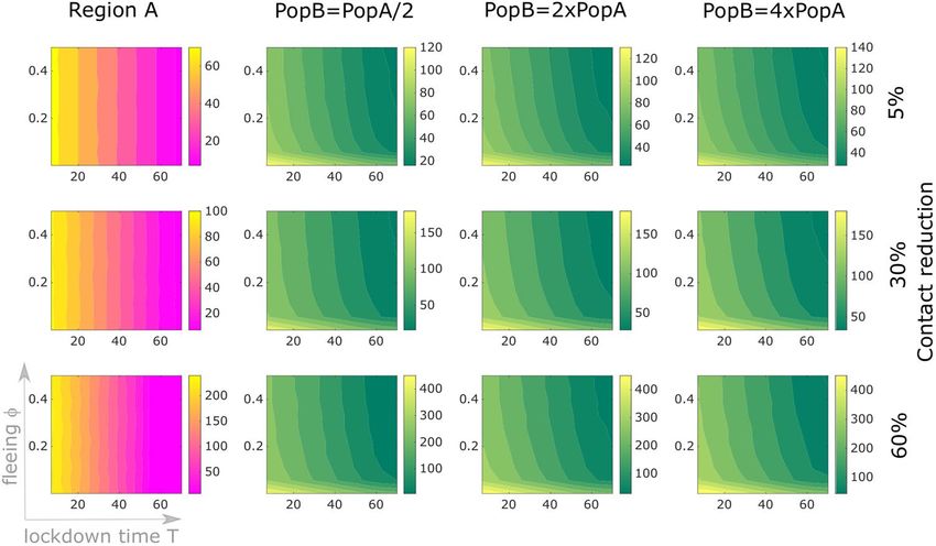
www.nature.com/scientificreports/
Lau et al.9, Lai et al.10, Boldog et al.11) investigate the association between the domestic/international travel load
and the number of cases exported from Wuhan to other regions in China. These studies, however, do not seem
to consider the large exodus induced by the lockdown measures.
We present here a mathematical framework for studying the effects of a potential lockdown-induced exo-
dus, together with the time and strength of intervention measures, on the outbreak size in different geographic
regions. We assume that the outbreak starts in one specific area, simply denoted as region A, where lockdown is
implemented at time T. This induces people from region A to flee the lockdown and move to another geographic
region B. If region B was disease-free up to time T, the lockdown-induced migration from region A can lead to
importation of the infection in a previously uninfected area. We formulate and study a compartmental epidemic
model for the spread of an infectious disease in the two different geographic regions, establishing a new type of
intervention-dependent final size relation. The latter can be used to estimate the final epidemic size even in the
case of a change in the population size due to the migration just before the lockdown. This model is calibrated
on the example of the Italian outbreak. By means of numerical simulations we project different scenarios show-
ing that (i) timely and stricter intervention could have significantly lowered the number of cumulative cases in
Italy, and (ii) migration of at the time of lockdown possibly played a minor role in the spread of the disease in
the country. The approach presented in this study can be adapted to describe the spread of an infectious disease
over multiple geographic regions or to describe the transmission of viruses others than SARS-CoV-2.
Methods
Modeling transmission dynamics. The mathematical model proposed in this study is based on a system
of ordinary differential equations (ODEs) that describes interactions between different groups of individuals in
the population. The proposed approach extends the known S-E-I-R (susceptibles–exposed–infected–recovered)
model for disease dynamics12, and is suitable to describe the spread of several infectious diseases, though we
shall specifically talk about COVID-19 later. Before describing the lockdown scenario and other intervention
measures aimed at mitigating the outbreak, we introduce the core model for the (uncontrolled) spread of the
virus in a population. The ODE approach that we use assumes that the population is homogeneous and well-
mixed within a region. Individuals are classified according to their status with respect to the virus spread in the
community.
At the beginning of the epidemic, that is, when first cases are reported, the majority of the population is
assumed to be susceptible (S), and hence can be infected. The time between exposure to the virus (becoming
infected) and symptom onset, on average 1/α days, is known as “exposed” or “presymptomatic” period. To better
understand the role of transmission from infected people with mild or no symptoms, we distinguish between
transmission from people who are infected, might have very mild symptoms, but remain undetected (U) and
transmission from people who are infected but still in the presymptomatic period (E). Detected infectives might
require hospitalization (H) or not (I). Detection of cases is assumed to occur either after the latent phase (with
probability ρ ) or post mortem (with probability σ ). Duration of infection can be different for the three different
groups. Undetected infections lead to undetected recoveries, which cannot be reported unless testing for ongo-
ing (virus detection) or previous (antibody detection) infections is performed. Individuals who recovered from
a detected (R) or an undetected ( RU ) infection, as well as patients who died from the infection (D), are removed
from the chain of transmission. Separation of the compartments R and RU allows to keep track of how many
people have recovered from infection without having been detected. At the same time, it is possible to use R(t)
for model calibration, when time series for recovered infectives are sufficiently reliable. Susceptible individuals
can be infected via contacts with presymptomatic (transmission rate βE ), undetected cases (transmission rate
βU ), detected but not hospitalized (βI ) and hospitalized cases (βH ). We assume that undetected infectives, due
to possibly absent or unspecific symptoms, do not restrict their contacts to others, and therefore have higher
transmission rates than detected infected individuals. Hospitalized cases are properly isolated, and hence their
transmission rate is assumed to be the lowest. The interpretation of model parameters, all assumed to be non-
negative, is summarized in Table 1. The dynamics of the core model described above and shown in Fig. 1 is given
by the following system of differential equations:
Ṡ(t) = − (t)S(t) susceptibles,
Ė(t) = (t)S(t) − αE(t) exposed/presymptomatic,
U̇(t) = (1 − ρ)αE(t) − γU U(t) undetected infectives,
İ(t) = ραE(t) − (γI + δI + η)I(t) detected, non-hospitalized infectives,
(1)
Ḣ(t) = ηI(t) − (γH + δH )H(t) hospitalized infectives,
Ṙ(t) = γI I(t) + γH H(t) recovered from detected infection,
ṘU (t) = (1 − σ )γU U(t) recovered from undetected infection,
Ḋ(t) = δI I(t) + δH H(t) + σ γU U(t) deceased,
where
βE E(t)+βI I(t) + βU U(t) + βH H(t)
(t) = ,
N(t)
Scientific Reports | (2021) 11:9233 | https://doi.org/10.1038/s41598-021-88204-9 2
Vol:.(1234567890)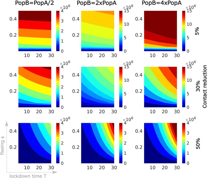
www.nature.com/scientificreports/
Parameters Description (unit)
βE Transmission rate from presymptomatics to susceptibles (1/(days × contact))
βU Transmission rate from undetected infectives to susceptibles (1/(days × contact))
βI Transmission rate from non-hospitalized cases to susceptibles (1/(days × contact))
βH Transmission rate from hospitalized cases to susceptibles (1/(days × contact))
1/α Duration of latency period (days)
γU Recovery rate for undetected infectives (1/days)
γI Recovery rate for non-hospitalized cases (1/days)
γH Recovery rate for hospitalized cases (1/days)
ρ Probability of detection on symptoms onset
σ Probability of detection post mortem
η Hospitalization rate (1/days)
δI Disease-induced death rate for non-hospitalized cases (1/days)
δH Disease-induced death rate for hospitalized cases (1/days)
φ Fraction of unconstrained population migrating from region A to region B
T Time of lockdown of region A
Table 1. Interpretation of model parameters.
Figure 1. Model structure for the transmission dynamics of an infectious disease, on the example of
COVID-19. Solid arrows indicate transition from one compartment to another, dashed arrows indicate
virus transmission due to contact with infectives. Upon infection, susceptible (S) individuals enter a latent/
presymptomatic phase (E). After symptoms onset, infections may be detected (I) or remain undetected (U).
Detected cases might become severe and require hospitalization (H). Infected individuals who recovered from
a detected (R) or an undetected (RU ) infection, as well as patients who died (D) upon infections, are removed
from the chain of transmission.
and N(t) = N0 − D(t), N0 being the total initial population at the beginning of the outbreak. That is,
N(t) = S(t) + E(t) + U(t) + I(t) + H(t) + R(t) + RU (t) is the current “effective” population at time t. Demo-
graphic variations other than disease-induced deaths are not considered in this work.
Numerical integration, model calibration and sensitivity analysis. The functionalities for solv-
ing the epidemic model (1) and fitting the parameters to the data were implemented in Python language: we
use odeint function from the scipy.integrate package13 for integrating the model equations and the
non-linear least-squares minimization from the lmfit module14 for estimating the parameters. We selected the
L-BFGS-B method15 for the optimization procedure, which is a very efficient algorithm for solving large scale
problems. In case the time series were incomplete, the days corresponding to the missing values were omitted
in the minimization. For all methods, we used the default values for options such as tolerances and step sizes.
The confidence intervals of the estimated model parameters were computed based on the standard error of the
estimated covariance matrix. For the plots in Figs. 2, 3, 4, and 5, integration in MATLAB ® by means of available
ODE routines (ode45, ode23s) was used. Numerical approximation of the final size formula was verified
by comparing the numerical solution of the implicit equation (4) (computed using fsolve from the scipy.
optimize package) with the numerical integration of the ODE model (1) over a sufficiently long time interval
(cf. Supplementary Material). Parameter sensitivity analysis of model quantities of interest, such as the basic
reproduction number, the number of hospitalized cases at the outbreak peak and the final size, were investigated
by means of Partial Rank Correlation Coefficients (PRCC) analysis 16. Latin Hypercube Sampling 17 was used
Scientific Reports | (2021) 11:9233 | https://doi.org/10.1038/s41598-021-88204-9 3
Vol.:(0123456789)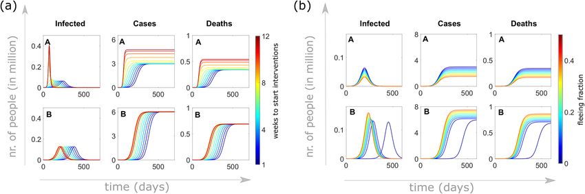
www.nature.com/scientificreports/
Figure 2. Detected infected cases and deaths depending on (a) the lockdown time T and (b) the fleeing fraction
of exposed/undetected individuals at the time of the lockdown. An initial outbreak starts off with 20 cases and
two deaths in region A (population 25 million), where lockdown is established at time T, immediately followed
by lockdown-induced migration of a fraction of the unconstrained population from region A to the disease-
free region B (population 50 million). (a) The lockdown time T varies from one to twelve weeks after the initial
reporting, while the fleeing fraction is fixed to 1% of the unconstrained population in region A; (b) 0.01% to
50% of the unconstrained population moves from region A to region B at the fixed time T = 21 days after the
initial reporting. At the time of lockdown, control measures are applied in both regions in order to restrict
contacts by 60% and reduce transmission.
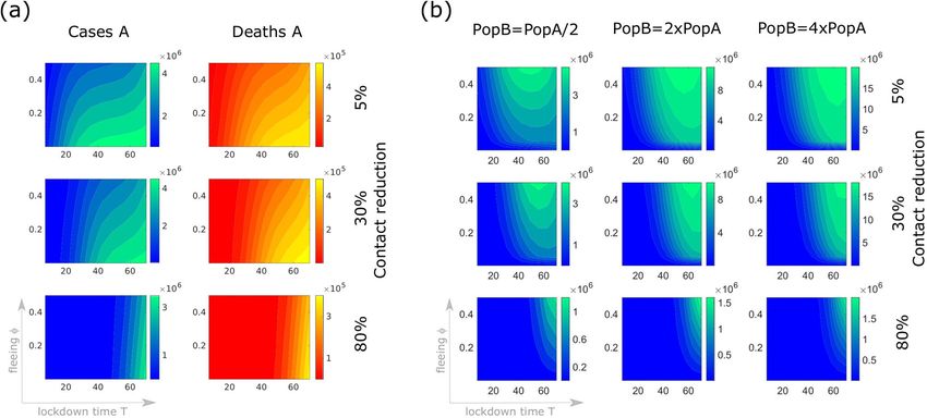
Figure 3. Sensitivity of cases in region B depending on the lockdown time T , the fraction φ of population
leaving region A, the strength of intervention measures in reducing contacts, and the population size of region
B. An initial outbreak starts off with 20 detected cases and two deaths in region A (population 25 million) which
is locked at time T (horizontal axes indicate days after the initial reporting) and lockdown-induced migration
(vertical axes) occurs. At the time of lockdown, control measures are applied to restrict contacts by 5% (first
row), 30% (second row) or 80% (third row), and maintained for two months. Color codes represent cases/deaths
projected at the end of the two months following model (1): (a) the number of detected cases (left column)
and deaths (right column) in region A, (b) detected case numbers in region B depending on the size of the
population in region B with respect to that of region A (columns).
to generate a representative sample set of tuples of parameters from the parameter ranges indicated in the Sup-
plementary Material. Using PRCC, we can rank the effect that each parameter has on the outcome, when other
parameters are simultaneously varying in the given ranges. Calculation of PRCC allows us to determine the
strength of statistical relationships that exist between each input parameter and the output variable. Parameters
with PRCC larger (respectively, smaller) than zero are positively (respectively, negatively) correlated with the
quantity of interest.
Scientific Reports | (2021) 11:9233 | https://doi.org/10.1038/s41598-021-88204-9 4
Vol:.(1234567890)www.nature.com/scientificreports/
Figure 4. How long should control measures be in place? An initial outbreak starts off with 20 cases and two
deaths in region A (population 25 million) which is then locked at time T (horizontal axes indicate days after
the initial reporting) and lockdown-induced migration (vertical axes) occurs. In both regions, at the time of
lockdown, control measures are applied to restrict contacts by 5% (first row), 30% (second row) or 60% (third
row), and maintained for 7 days after the peak in the daily incidence in the respective region is reached. Color
codes represent the duration in days of the control period in region A (first column) and region B (second
to fourth columns), also depending on the population size in region B (being half, twice or four times the
population in region A).
Results
Reproduction number. Possibly among the most interesting quantities to identify in the early phase of an
outbreak, the basic reproduction number (denoted by R0) is used in mathematical epidemiology as an indicator
for the transmissibility of the disease. This R0 is a metric which indicates the average number of secondary infec-
tions generated in a fully susceptible population by one infected host over the course of the infection. In most
epidemiological models, R0 > 1 leads to a disease outbreak, whereas for R0 < 1 the disease will not spread in
the population.
The basic reproduction number of system (1) can be calculated analytically (cf. Supplementary Material),
e.g., by means of the next-generation matrix approach18, and is given by
βE ρβI ρβH η βU (1 − ρ)
R0 = + + + .
α γ + δ + η (γI + δI + η)(γH + δH ) γU (2)
I
I
=:RE0 =:RI0 =:RH =:RU
0 0
The summands of R0 account for contacts with presymptomatic cases ( RE0 ), undetected infectives ( RU 0 ),
detected non-hospitalized ( RI0 ) and hospitalized ( RH 0 ) cases. The reproduction number evolves in time with
time-dependent parameters, which might vary e.g. because of intervention measures, and with variations in
the susceptible portion of the population. As the outbreak evolves, people who go through infection are either
immunized or die, and the susceptible population decreases (vaccination-induced immunity is not considered
here but would also contribute to lowering the susceptible population). The effective reproduction number Rt
at time t can be obtained by the same formula, substituting the values of time-dependent parameters in (2) and
multiplying this value by the susceptible fraction of the population, S(t)/N(t). The reproduction number can be
controlled via intervention measures aiming not only at reducing transmission, but also at improving detection,
or at enhancing isolation and treatment of infectives. Figure S1 in the Supplementary Material shows that the
reproduction number can be most effectively controlled via regulation of transmission rates.
Modeling the lockdown at time T and migration from region A. Inspired by the history of the
COVID-19 outbreak in China and Italy, we use the previously presented transmission network (1) to describe
an outbreak spreading from one geographic region A, to the rest of the country (here considered as one single
region, B). The country itself is assumed to be isolated, that is, migration inward/outward is not considered here.
The outbreak is assumed to have started in region A, that is, numerous cases were detected in a short time during
the early phase of the epidemic. The prevalence (cases/population) of COVID-19 in region A being much higher
than in the rest of the country (region B), the government decides that region A is going to be confined at some
time T. This motivates many people to move from region A to region B, just before region A is effectively isolated
from the rest of the country. We adapt the mathematical model (1) to reproduce this situation and understand
how the lockdown time T, and the migration of a fraction φ ∈ (0, 1) of the unconstrained population (that is,
Scientific Reports | (2021) 11:9233 | https://doi.org/10.1038/s41598-021-88204-9 5
Vol.:(0123456789)www.nature.com/scientificreports/
Figure 5. Cumulative detected cases in region B three months after lockdown of region A depending on the
fraction φ of population leaving region A, the intervention time TB in region B, the effectiveness of intervention
measures in reducing contacts, and the population size of region B. Region A is isolated 21 days after the
beginning of the outbreak and migration towards region B occurs. For each panel, the vertical axis denotes the
variation in the fleeing fraction from A (φ, between 0.1% and 0.5). On the horizontal axis, the reaction time
TB indicates how many days passed for control measures in region B to be applied since isolation of region A.
Control measures are applied in region B to restrict contacts by 5% (first row), 30% (second row) or 50% (third
row), and maintained until the end of the simulations. Cumulative detected cases are projected also depending
on the size of population in region B with respect to that in region A (columns). Note the different scaling of the
color legend in the panels.
everyone except detected, hospitalized and deceased persons) from region A to region B could affect the evolu-
tion of the epidemic in the two regions. Detected cases, hospitalized cases and deceased individuals, cannot leave
region A at any time. Transitions between region A and region B, which are assumed to be in balance before the
lockdown, are stopped after time T. Migration is modeled as an impulse at time T, simplifying a possible contin-
uous transition from A to B in the days immediately ahead the lockdown. This means we impose the conditions
B
Z (T+ ) = φZ A (T− ) + Z B (T− )
for Z = S, E, U, R, RU , and
Z A (T+ ) = (1 − φ)Z A (T− ) (3)
j j
[0.1cm] X (T+ ) = X (T− ), where X = I, H, D, j = A, B,
where T− denotes the time just before migration occurred and and T+ denotes the time of migration, respectively.
After the lockdown (t ≥ T ) the outbreak evolves independently in the two regions. Further, concurrent with
the lockdown, other non-pharmaceutical intervention measures, such as encouraged social distancing, school
closure, shut down of many economic activities, increased testing activity, improved hospital capacity etc., might
be introduced in both regions, possibly in a different manner or with different timing.
Final size. The final size relation is an analytic formula to predict the total number of individuals in the pop-
ulation who are infected over the course of the epidemic12. By means of analytical methods (cf. Supplementary
Material), we derived a final size relation taking into account the lockdown time (T) and the induced exodus at
the time of the lockdown. This formula provides a reliable approximation of the cumulative cases, when the total
population and the parameters do not vary too much after time T. Assume the status of the system, including
the numbers of cases, hospitalizations, deaths, recoveries, and active population ( N ), in one region right after
Scientific Reports | (2021) 11:9233 | https://doi.org/10.1038/s41598-021-88204-9 6
Vol:.(1234567890)www.nature.com/scientificreports/
the lockdown time (denoted below by the subscript T +) can be obtained from available data or approximated by
means of the model (1). Then the final size formula
ln ST + − ln S∞ = �(N − S∞ ) + b̃1 (χ − 1)IT + + (χ − 1)b̃2 HT +
+ χ(b̃3 − ã4 ) + � − b̃3 DT + (4)
+ (χ(b̃4 − ã2 ) − b̃4 )RT + − χ ã1 UT + − χ ã3 RTU+ ,
allows us to determine the number of cases occurring over the complete course of the outbreak, without requir-
ing model integration after time T. Observe that the fleeing ( φ ) is included in the relation (4) into N and
the terms with T + −subscript, following the conditions (3). Here S∞ denotes the portion of population which
remains susceptible at the end of the outbreak. If S0 ≈ N0 is the susceptible (total) population at the beginning
of the outbreak, then S0 − S∞ corresponds to the cumulative number of cases at the end of the outbreak. The
coefficients χ, �, ãj , b̃j , j = 1, . . . , 4 in equation (4) are obtained from the parameters of model (1) as detailed
in the Supplementary Material. Formula (4) is used below to analyze the sensitivity of the total number of cases
with respect to model parameters.
How lockdown and intervention measures affect the evolution of the outbreak. The proposed
model (1) with the lockdown scenario (cf. “Methods”) is used to investigate the sensitivity of case and death
counts with respect to the intervention parameters, such as the time of lockdown of the source region A, the
fraction of population fleeing region A due to the lockdown announcement, and the strength and timing of
intervention measures in both regions. We consider a hypothetical scenario which is suitable to describe various
infectious diseases and populations, though inspired by COVID-19 spreading in a fully susceptible population.
Region A, where the outbreak starts, is assumed to have a population of 25 million. Though the population size
in region B can vary, this region is always assumed to be disease-free until lockdown of region A occurs. Region
B is parametrized as region A, unless explicitly mentioned. We set the parameter values such that the initial
reproduction number in region A is R0 ≈ 3.8, while the beginning of the outbreak is defined to occur with 20
cumulative detected cases and two deaths. For further details on the parametrization used for this section, we
refer to the Supplementary Material.
Figure 2a shows how the cumulative number of detected cases and deaths depend on the lockdown time T.
At the time of lockdown, which varies here between one and twelve weeks after the beginning of the outbreak
in region A, 1% of the unconstrained population flees from region A to region B. Lockdown is coupled with
stronger control measures, both in region A and region B, which assume reduction in contact rates by 60% to be
maintained until the end of the observations (here about two years after beginning of the outbreak). This reduces
the reproduction number in both regions, but not enough to prevent an outbreak also in region B (RBT ≈ 1.5).
The panels in Fig. 2a show that in both regions, the time of the lockdown strongly affects both the number of
cases and the peak of the epidemic wave. Figure 2b shows the cumulative number of detected cases and deaths,
depending on the fraction of exposed and undetected infected individuals leaving region A for region B. Here
the lockdown time T is fixed at three weeks after the beginning of the outbreak, whereas the migrating popu-
lation φ varies (between 0.01% and 50% of the unconstrained population in region A at the lockdown time).
Increasing the fleeing fraction φ , the peak in cases decreases in region A, whereas in region B, it increases and
advances in time.
Figure 3a shows the variation in cumulative detected cases and deaths in region A depending on the lockdown
time T, the fraction φ of population leaving region A and the effectiveness of intervention measures in reducing
contacts. We project here the number of cases and deaths predicted by the model two months after lockdown,
while control measures are maintained for the whole period. While migration does not particularly affect the
evolution of the outbreak in region A in case of early intervention, the later the lockdown and the weaker the
control measures, the higher will be the number of cases and deaths. In case of late lockdown time (about two
months after the beginning of the outbreak), a significant fleeing population reduces the number of cases/deaths
in region A, in agreement with what observed in Fig. 2. Opposite is the effect of migration from region A on
cumulative cases (and deaths, not shown here) in region B. Fig. 3b shows the importance of applying stronger
control measures in region B when region A is locked. When contact restrictions are more severe, the size of
the population of region B does not importantly affect the outcome of the outbreak. If contact restriction is
minimal in region B, a higher populated target region allows a longer and more dramatic outbreak (with more
cases and more deaths).
One of the most difficult questions to answer during an ongoing epidemic concerns the duration of restrictive
control measures. How long should these restrictions be in place? Several criteria could be applied to determine
the end of the restrictive measures19. Here we assume that a region is released one week after reaching the peak
in the daily incidence of reported cases. As in the above simulations, we assume that the outbreak spreads from
region A to region B when the former is isolated. The result is shown in Fig. 4. In both regions, at the time of
lockdown, control measures are applied to restrict contacts by 5% to 60%, and maintained for 7 days after the
peak in the daily incidence in the respective region is reached. More restrictive measures postpone (and lower,
cf. Fig. 3b) the peak of the outbreak, however this prolongs the time that the control measures should be in place.
On the other hand, migration and late intervention accelerate the speed of the epidemic in region B, and hence
the peak comes earlier (is much higher, brings more cases and more deaths, cf. Fig. 2) and makes the lockdown
time shorter.
So far we have assumed that control measures in region B are applied when region A is isolated. Figure 5
illustrates the damage that could be induced by a delayed reaction in region B combined with the application
Scientific Reports | (2021) 11:9233 | https://doi.org/10.1038/s41598-021-88204-9 7
Vol.:(0123456789)www.nature.com/scientificreports/
of not sufficiently strong control measures. The panels show the number of cases in region B three months after
lockdown of region A occurred (here T is fixed on day 21 since the beginning of the outbreak), assuming that
the interventions in region B is delayed by TB days with respect to region A.
COVID‑19 in Italy as an example
In the previous section we used the model (1) to study the spread of a potential outbreak on two hypothetical
geographic regions, without specific application to real data. Here we consider the recent COVID-19 outbreak in
Italy and apply model (1) to study the lockdown and the early outbreak dynamics. The COVID-19 outbreak hit
Italy in early 2020 as the first country in Europe. While preliminary control measures were introduced locally at
the end of February as first cases were detected, at the beginning of March a large area including Lombardy and
several provinces in Emilia-Romagna, Veneto, Piedmont and Marche were declared as “red zone” and i solated20.
Shortly after, even more restrictive control measures were applied on the whole country3.
Data and setting for parametrization. The publicly available data-set provided by the Italian Ministry
of Health (Ministero della Salute) and the national Civil Protection Department (Dipartimento della Protezi-
one Civile)21 was used for this study. Time series for hospitalized (totale_ospedalizzati), daily case incidence
(nuovi_positivi) and cumulative cases (totale_casi), as well as deaths (deceduti) were obtained from the dati-
regioni repository21. Data for region A was prepared accounting for the isolated provinces3,22. As hospitalization
and death counts are available at regional level, but not at the level of provinces, we define region A as the area
composed of the whole regions of Lombardy, Emilia-Romagna, Veneto, Piedmont and Marche (about 25 mil-
lion people). In reality, only fourteen largely-neighboring provinces in Emilia-Romagna, Veneto, Piedmont and
Marche were isolated, together with Lombardy which is the most populous region in Italy and accounts for the
majority of COVID-19 cases. Region B is defined as the rest of the country (about 35 million people). The model
is calibrated on daily incidence, deaths and hospitalized time series for the two regions. Based on estimates from
previous studies, we fix the average duration of the latent phase (1/α ≈ 5.5 days23,24), and the duration of the
infectious periods in undetected (ca. 7 days24,25) and in detected cases (ca. 10 days26,27). For model parameters
that cannot be obtained from other references nor estimated reliably with the available data, we fix values based
on plausible assumptions. For example, we fix the ratio between βE (respectively, βI and βH ) and βU and esti-
mate the latter. It is unclear which amount of secondary cases resulted from presymptomatic transmission, with
estimates ranging from 6.4%28 to 44%29. Here we assume that βE = 0.2βU , accounting for a two days infectious
period in the presymptomatic phase. As undetected infectives have possibly mild or no symptoms, we assume
that they do not restrict their contacts to others, and therefore have higher transmission rates than detected
cases (βI = 0.25βU ). Hospitalized patients are supposed to have very limited contacts compared to undetected
cases (βH = 0.1βU ). The detection ratio ρ is estimated based on Table 1 of the very recent report by the Italian
National Institute of Statistics and the Ministry of Health on the seroprevalence in Italy30. From the data shown
in this report, we could compute a seroprevalence 4.53% (weighted average) for region A and 0.96% for region
B, as of July 20, 2020. As of the same date, the cumulative cases in region A and region B report about 182,000
cases detected in region A and about 62,000 cases detected in region B 21. Rounding the seroprevalence to 5% for
region A, this leads to 1.25 million estimated COVID-19 cases for region A, out of which we know only 182,000,
henceforth a detection ratio ρA ≈ 14.5%. Analogously, rounding to 1% seroprevalence for region B, we obtain
ρB ≈ 17.5%. We assume that the detected cases are hospitalized with a rate η = pH /2, where the probability
pH ∈ (0, 1) of being hospitalized two days after symptoms onset is estimated from the data. Once the detected
cases are hospitalized, they are assumed to either recover with a probability pHR ∈ (0, 1) after 10 days, or die
with a probability (1 − pHR ). This leads to a recovery rate of γH = pH pHR /10 in the hospitals and a death rate
of δH = pH (1 − pHR )/10. The probability pHR is estimated from the data. Among those detected cases that do
not get hospitalized, we assume that pIR = 99% of the cases recover after on average 10 days from symptoms
onset, while the remaining 1% die. This means that we can interpret the recovery rate of the detected cases that
are not hospitalized as γI = (1 − pH )pIR /10 and the death rate as δI = (1 − pH )(1 − pIR )/10. We assume that
σ = 0.1% cases are detected post mortem.
The initial time point for simulations is set to February 24, 2020. Most of the initial conditions for solving the
ODE system, such as the number of deaths or hospitalized cases could be obtained directly from the data. How-
ever, there is no data available for the exposed and undetected infections. These values are approximated making
use of the detection ratio ρ and the average latency period 1/α, with ρE(0) roughly corresponding to the case
incidence six days later, and U(0) corresponding to the undetected fraction (1/ρ − 1)I(0) of cases at the begin-
ning of the observations. The initial conditions used for simulations are specified in the Supplementary Material.
To parametrize model (1) taking into account the numerous intervention measures adopted in the early
phase of the outbreak we define three time periods: before lockdown (February 24–March 8), under initial
lockdown measures (March 9–21) and under stricter lockdown measures introduced later (March 22 – May 4).
At the lockdown time T (March 9), we assume that 0.5% (φ = 0.005) of the unconstrained population in region
A (roughly 130,000 people) migrate to region B. Given the available data, the parameter φ cannot otherwise be
reliably estimated. Nevertheless, the estimated number is plausible, given the reported large migration from the
north of the c ountry5,6. The model parameters for the two regions were estimated for each time period indepen-
dently. When available, the estimated parameters from the previous time period were given as initial guesses
for the optimizer in the next time period. The estimated and fixed model parameters for the three time periods
are summarized in the Supplementary Material. The result of the model fit is given in Figure 6. The parameter
estimation results highlight a clear reduction in the contact rates (βU ), lowering the basic reproduction number
in region A from R0 = 3.7 at the beginning of the outbreak to Rt = 0.76 at the end of March, in agreement with
estimates obtained by other groups31. The decrease in the hospitalization rate η and increase in the mortality
Scientific Reports | (2021) 11:9233 | https://doi.org/10.1038/s41598-021-88204-9 8
Vol:.(1234567890)www.nature.com/scientificreports/
Figure 6. Model fit for the early dynamics of the COVID-19 outbreak in Italy. Reported data (dots) and model
results (crosses) for daily incidence (left panel), deaths (middle panel) and hospitalized cases (right panel) in
region A (Lombardy, Emilia-Romagna, Marche, Piedmont, Veneto; red) and region B (rest of the country; blue).
Parameter values are estimated as indicated in three different time intervals (separated by vertical lines in the
figure): pre-lockdown (February 24–March 8), first lockdown measures (March 9–21), and extended lockdown
measures (March 22–May 4), cf. Supplementary Material.
Figure 7. Scenario comparison for (a) the cumulative cases of COVID-19 in Italy as of May 4, 2020, and
(b) evolution in time of susceptibles, detected and hospitalized cases, and deaths until the release of control
measures on May 4, 2020. Simulations show the populations in region A and region B for different scenarios:
(baseline, blue curves) the setting as of fit in Fig. 6; For all other scenarios severe restrictions (parameter set as
of March 22) are in place from the lockdown time: (SC2) lockdown on March 9 (SC2a, red) with and (SC2b,
yellow) without fleeing population at lockdown; (SC3) lockdown anticipated to March 2 (SC3a, magenta) with
and (SC3b, green) without fleeing population at lockdown.
rates δI , δH can be explained with the quickly rising number of hospitalizations and deaths in the second half of
March and beginning of April. Fitting data for both region A and region B, we clearly see that control measures
were effectively in place also in region B, in which the reproduction number was also lowered to Rt = 0.7 at the
end of March. Compared to the abstract scenarios considered in the previous section, we are here in a setting
where the population in region B is about 1.5 times larger than in region A, however not fully disease-free at the
time of the outbreak. First cases outside of region A were reported at the end of February, quickly isolated, and
could be traced back to clusters in Lombardy or V eneto3. While control measures were introduced more severely
in region A, awareness and other major interventions such as school closure were applied on the whole Italian
territory even before the lockdown on March 9. After May 4, the lockdown was released and most severe control
measures were relaxed in more steps. As the focus of this work was concerned with the isolation of a specific
region and not with the full parametrization of the ongoing outbreak, we do not consider here the relaxations
of the control measures, nor data after May 4. Starting from the obtained data-fit, we simulate different possible
scenarios for a hypothetical intervention with stricter and/or earlier measures. We compare (Fig. 7a) the number
Scientific Reports | (2021) 11:9233 | https://doi.org/10.1038/s41598-021-88204-9 9
Vol.:(0123456789)www.nature.com/scientificreports/
Figure 8. Partial rank correlation coefficients (PRCCs) of seven main model parameters for (a) reproduction
number, (b) final size (S∞) and (c) the number of hospitalized cases at peak in region A. Parameters with PRCC
larger than zero are positively correlated with the quantity of interest, whereas parameters with negative PRCC
are negatively correlated. Parameters were varied within the ranges given in the Supplementary Material.
of cumulative cases in region A and region B as of May 4 for different scenarios, with baseline representing the
parameter setting as of the fit in Fig. 6. For all other scenarios we assume that most severe restrictions (param-
eter set as of March 22, cf. Supplementary Material) are in place from the lockdown time. In scenario 2 (SC2)
we keep the lockdown time as for the data fit and assume that strict intervention measures are in place from
March 9, whereas in scenario 3 (SC3) we advance the lockdown by one week to March 2. In both scenarios we
consider a fraction (0.5%) of unconstrained individuals (a) to not flee (b) to flee region A immediately before
the lockdown. Figure 7b reports the evolution in time of different compartments in region A and B. As the flee-
ing rate is assumed homogeneous among compartments (cf. condition (3)), the migration from region A to
region B is most evident in the susceptible population, which at the time of the lockdown is yet very large. The
projected scenarios show that stricter interventions from the beginning of the lockdown could have reduced the
number of cumulative cases as of May 4 by at least one third, and that importation of cases has far less impact
than timely intervention.
Sensitivity analysis. To quantify the effect that model parameters, in particular those which might be
affected by control measures, have on critical quantities of the epidemic, we performed a global sensitivity analy-
sis using PRCC on seven model parameters (cf. “Methods” and Supplementary Material). Figure 8 shows the
result of the sensitivity analysis of the reproduction number R0, the final size (S∞) as of formula (4), and the
number of hospitalized cases at the outbreak peak in the target region A (analogous results for region B, not
shown here). Panels in Fig. 8 show that βU and ρ have the strongest correlation with all the three model outputs.
Therefore, a small increase in the transmission rate of undetected cases or a small decrease in the detection ratio
can significantly increase the spread of the disease (R0) and the number of hospitalized cases at the outbreak
peak eventually leaving much fewer susceptibles in the population at the end of the epidemic (S∞). Recovery,
hospitalization and death rates are negatively correlated with the reproduction number (positively with S∞).
The number of hospitalized cases at the outbreak peak is also strongly affected by the recovery rate for the H
compartment (γH ).
Discussion
A major epidemic outbreak might require authorities to introduce various control measures, from encouraging
social distancing to closing educational and economical activities. The goal is to limit the number of victims
and to prevent the health care system from collapsing. In the present study, we have established a model for the
spread of an epidemic outbreak considering the effects of an exodus of large masses of people from infected
areas before restrictive control measures are introduced. Such a phenomenon was reported in the occasion of the
COVID-19 outbreak, first in Wuhan, China and then in Northern Italy. The compartmental model introduced
in our work differentiates infected people based on the severity of their infection, accounting also for presymp-
tomatic transmission, undetected infections and hospitalized cases. We consider two geographic regions, with
the disease being initially confined in region A, where also strict control measures are applied and from where
people flee to a previously (ideally) uninfected region B. In contrast to previous studies for the spread of COVID-
19, we consider here the geographic distribution of cases, but relax the classification of the individuals into age
groups24,32,33. Calculating the basic reproduction number (2), we identified its four components that account
for transmissions from presymptomatic, undetected infectives, detected but not hospitalized, and hospitalized
cases. Further we have derived a new type of final size relation (4), a formula serving for the estimation of the
total number of infectives during the whole duration of the epidemic. A final size formula in nonautonomous
epidemic models was previously obtained, for example, in a model for Ebola Virus D isease34. The novelty in
this work is that the final size relation obtained here covers models in which not only the parameters, but also
the population size varies at some specific time point T (in the considered example due to a fleeing fraction of
individuals from one region to another). The result presented here is novel and flexible, so that it is suitable to
study various outbreaks of infectious diseases. Further, the same approach could be used for describing migration
out of region A and distribution of a fraction φi of individuals moving from region A to a region Bi , i = 1, . . . , n
for an arbitrary number n ∈ N of destination regions.
Scientific Reports | (2021) 11:9233 | https://doi.org/10.1038/s41598-021-88204-9 10
Vol:.(1234567890)www.nature.com/scientificreports/
By means of numerical simulations, we have assessed the short-term effect of various parameters on the
number of cases and the number of deaths. Figures 2, 3, 4 and 5 show that the earlier the lockdown happens, the
slower and less dramatic the epidemic evolves, in agreement with previous s tudies7–9. A late lockdown impor-
tantly advances the peak in the number of currently infected people and leads to significantly more deaths and
total cases. The fraction of people moving from region A to region B, however, rather affects the latter region.
The more individuals moving from region A to region B, the earlier the peak in the infective curve of the target
region. The strength and timing of intervention measures in region B is crucial to contain the number of cases
and deaths due to importation of the disease from region A (Fig. 3b). We have first assumed that control meas-
ures are applied at the same time of the lockdown both in region A and in region B, simulating the behavior of
people fleeing isolation and joining their relatives, rather than avoiding restrictive measures. Delays of up to a
month in intervention in region B, compared to the lockdown time of region A, can be balanced out with the
maintenance of stricter control measures also in region B. More restrictive measures postpone (and lower, cf.
Fig. 3b) the peak of the outbreak, however this prolongs the time intervention measure should be in place, if
reaching the peak of the infections curve is the criterion for controls to be relaxed.
As an example, we have fitted our model to the Italian COVID-19 data (Fig. 6), the most affected areas in the
country defining region A, and the rest of the country corresponding to region B. Projection of different scenarios
(Fig. 7) shows that timely and strict intervention could have importantly lowered the number of cumulative cases
(in region A by at least 60%) and that migration at the time of lockdown possibly played a minor role for the
spread of the disease in Italy. A limitation of our work is that in our setting, migration from region A to region
B is assumed to occur as an impulse at time T. Given the available data, the fleeing fraction ( φ ) could not be
reliably estimated and it was fixed to obtain a plausible value for the reported large migration from the north of
the country. While it was initially observed that a large number of people fled the quarantined regions immedi-
ately before these were confined, it is yet debated if the exodus was not rather diluted over the time starting on
February 2335. A repeated or continuous migration from region A to region B could be included in the model
simulations, though this would increase uncertainty in the parametrization. Similarly, the assumption that all
unconstrained compartments move in the same proportion from region A to region B could be relaxed, and
different fleeing scenarios could be assumed. In all cases, the final size formula (4) would still hold true, as long
as the parameters before/after intervention are known and the values for detected cases, hospitalized, recovered
and deceased people at time T can be estimated from the early outbreak data. In this study, we focused on the
timing and strength of intervention, but did not take into account relaxation of control measures. Our setting is
realistic for short-term intervention scenarios, such as two to three months, as was the case in many countries
during the COVID-19 pandemic. For long-term predictions, assuming maintenance of strict control measures
over several months leads to an unrealistically low estimate for the number of total cases and deaths.
Received: 14 September 2020; Accepted: 8 April 2021
References
1. BBC News. China coronavirus: Lockdown measures rise across Hubei province 23 January 2020. https://www.bbc.com/news/world-
asia-china-51217455. Last accessed 7 August 2020
2. Zhao, S. et al. Quantifying the association between domestic travel and the exportation of novel coronavirus (2019-nCoV) cases
from Wuhan, China in 2020: a correlational analysis. J. Travel Med. 27(2), taaa022 (2020).
3. Wikipedia. COVID-19 pandemic lockdown in Italy. https://en.wikipedia.org/wiki/COVID-19_pandemic_lockdown_in_Italy. Last
accessed 29 July 2020.
4. della Sera, C. Coronavirus, la grande fuga da Milano prima del decreto che isola la Lombardia 8 March 2020. https://www.corriere.
it/c ronac he/2 0_m
arzo_0 8/c orona virus-g rande-f uga-m
ilano-p
rima-d
ecret o-c he-i sola-l ombar dia-9 b87a1 5a-6 0df-1 1ea-8 d61-4 38e0
a276fc4.shtml. Last accessed 11 August 2020.
5. Stampa, L. Fuga dal Nord: ventimila persone rientrate in Sicilia nel weekend 11 March 2020. https://www.lastampa.it/topnews/
primo-piano/2020/03/11/news/fuga-dal-nord-ventimila-persone-rientrate-in-sicilia-nel-weekend-1.38580593. Last accessed 11
August 2020.
6. Stampa, L. In fuga dal Nord Italia, 11 mila individuati in Sardegna: per tutti scattata la quarantena obbligatoria 11 March 2020.
https://www.lastampa.it/cronaca/2020/03/11/news/in-fuga-dal-nord-italia-11-mila-individuati-in-sardegna-per-tutti-scattata-
la-quarantena-obbligatoria-1.38580219. Last accessed 11 August 2020.
7. Chen, Z.-L. et al. Distribution of the COVID-19 epidemic and correlation with population emigration from Wuhan. China. Chin.
Med. J. (Engl.) 133(9), 1044–1050 (2020).
8. Li, X., Zhao, X. & Sun, Y. The lockdown of Hubei Province causing different transmission dynamics of the novel coronavirus
(2019-nCoV) in Wuhan and Beijing. medRxiv, https://www.medrxiv.org/content/10.1101/2020.02.09.20021477v2 (2020)
9. Lau, H. et al. The positive impact of lockdown in Wuhan on containing the COVID-19 outbreak in China. J. Travel Med 27(3),
taaa037 (2020).
10. Lai, S. et al. Assessing spread risk of Wuhan novel coronavirus within and beyond China, January–April 2020: a travel network-
based modelling study. medRxiv, https://www.medrxiv.org/content/10.1101/2020.02.04.20020479v2 (2020).
11. Boldog, P. et al. Risk assessment of novel coronavirus COVID-19 outbreaks outside China. J. Clin. Med. 9(2), 571 (2020).
12. Brauer, F., Castillo-Chavez, C. & Feng, Z. Mathematical Models in Epidemiology (Springer, Berlin, 2019).
13. Virtanen, P. et al. SciPy 1.0: fundamental algorithms for scientific computing in Python. Nat. Methods 17.3, 261–272 (2020).
14. Newville, M. et al. lmfit/lmfit-py 1.0.1. Zenodo, https://zenodo.org/record/3814709. May 2020.
15. Zhu, C., Byrd, R. H., Lu, P. & Nocedal, J. Algorithm 778: L-BFGS-B: Fortran subroutines for large-scale bound-constrained opti-
mization. ACM T. Math. Software 23(4), 550–560 (1997).
16. Blower, S. M. & Dowlatabadi, H. Sensitivity and uncertainty analysis of complex models of disease transmission: an HIV model,
as an example. Int. Stat. Rev./Revue Internationale de Statistique 62, 229–243 (1994).
17. Mckay, M. D., Beckman, R. J. & Conover, W. J. A comparison of three methods for selecting values of input variables in the analysis
of output from a computer code. Technometrics 42(1), 55–61 (2000).
Scientific Reports | (2021) 11:9233 | https://doi.org/10.1038/s41598-021-88204-9 11
Vol.:(0123456789)www.nature.com/scientificreports/
18. Diekmann, O., Heesterbeek, J. A. P. & Roberts, M. G. The construction of next-generation matrices for compartmental epidemic
models. J. R. Soc. Interface 7, 873–885 (2010).
19. Rawson, T., Brewer, T., Veltcheva, D., Huntingford, C. & Bonsall, M. B. How and when to end the COVID-19 lockdown: an opti-
mization approach. Front. Public Health 8, 262 (2020).
20. Davidson, H., Tondo, L. & Yu, V. Coronavirus: quarter of Italy’s population put in quarantine as virus reaches Washington DC. The
Guardian, 8 March 2020. https://www.theguardian.com/world/2020/mar/08/coronavirus-italy-quarantine-virus-reaches-washi
ngton-dc. Last accessed 13 August 2020.
21. Dipartimento della Protezione Civile. Dati COVID-19 Italia. https://g ithub.c om/p cm-d pc/C
OVID-1 9. Last accessed 4 August 2020.
22. La Repubblica. Stretta del governo, Lombardia e 14 province in isolamento. Conte: “Cambiare lo stile di vita”. Speranza: “Pugno duro
contro gli irresponsabili” 8 March 2020. https://w ww.r epubb
lica.i t/c ronac a/2 020/0 3/0 7/n ews/c orona virus_c hiusa_l a_l ombar dia_e_
11_province_-250570150/?ref=RHPPTP-BH-I250571072-C12-P2-S1.12-T1. Accessed 29 July 2020.
23. an der Heiden, M. & Hamouda, O. Schätzung der aktuellen Entwicklung der SARS-CoV-2-Epidemie in Deutschland – Nowcasting.
Epi. Bull. 17 (2020).
24. Barbarossa, M. V. et al. Modeling the spread of COVID-19 in Germany: early assessment and possible scenarios. PLoS ONE 15(9),
e0238559 (2020).
25. Prem, K. et al. The effect of control strategies to reduce social mixing on outcomes of the COVID-19 epidemic in Wuhan, China:
a modelling study. Lancet Public Health 5(5), e261–e270 (2020).
26. Wöfel, R. et al. Virological assessment of hospitalized patients with COVID-2019. Nature 581(7809), 465–469 (2020).
27. RKI. SARS-CoV-2 Steckbrief zur Coronavirus-Krankheit-2019 (COVID-19) Robert Koch-Institute, Berlin, Germany 2020. https://www.
rki.de/DE/Content/InfAZ/N/Neuartiges_Coronavirus/Steckbrief.html#doc13776792bodyText11. Last accessed 11 August 2020.
28. Wei, W. E. et al. Presymptomatic Transmission of SARS-CoV-2–Singapore, January 23–March 16, 2020. MMWR 69(14), 411
(2020).
29. He, X. et al. Temporal dynamics in viral shedding and transmissibility of COVID-19. Nat Med. 26(5), 672–675 (2020).
30. Istat – Ministero della Salute. Indagine di sieroprevalenza sul SARS-CoV-2, Anno 2020 (dati provvisori) available online, Aug 3,
2020. https://www.istat.it/it/files//2020/08/ReportPrimiRisultatiIndagineSiero.pdf
31. Guzzetta, G. et al. The impact of a nation-wide lockdown on COVID-19 transmissibility in Italy. arXiv, 2004.12338 (2020).
32. Weitz, J. S. et al. Modeling shield immunity to reduce COVID-19 epidemic spread. Nat. Med. 26, 849–854 (2020).
33. Röst, G. et al. Early phase of the COVID-19 outbreak in Hungary and post-lockdown scenarios. Viruses 12(7), 708. https://doi.
org/10.3390/v12070708 (2020).
34. Barbarossa, M. V. et al. Transmission dynamics and final epidemic size of Ebola virus disease outbreaks with varying interventions.
PLOS ONE 10(7), e0131398 (2015).
35. D’Alessandro, J. Coronavirus, l’illusione della grande fuga da Milano. Ecco i veri numeri degli spostamenti verso sud. La Repub-
blica, 23 April 2020. Last accessed 8 July 2020.
Acknowledgements
The work of MVB was supported by the LOEWE focus CMMS. AD was supported by the grant NKFIH PD
128363 and the János Bolyai Research Scholarship of HAS. NB was supported by the grant EFOP-3.6.2-16-2017-
00015 and ZsV by the grant NKFIH KKP 129877. The work of GR was supported by NKFIH FK 124016 and
TUDFO/47138-1/2019-ITM.
Author contributions
Conceptualization: MVB, GR; Modeling: MVB, GR; Mathematical analysis: MVB, AD; Data curation and analy-
sis: NB, HVV; Literature research: AD, MVB, HVV; Software development: ZV, NB, HVV; Calibration: HVV.
Numerical simulations: HVV, ZV, MVB. Writing (original draft): MVB, AD.
Funding
Open Access funding enabled and organized by Projekt DEAL.
Competing interests
The authors declare no competing interests.
Additional information
Supplementary information is available for this paper at https://doi.org/10.1038/s41598-021-88204-9.
Correspondence and requests for materials should be addressed to M.V.B.
Reprints and permissions information is available at www.nature.com/reprints.
Publisher’s note Springer Nature remains neutral with regard to jurisdictional claims in published maps and
institutional affiliations.
Open Access This article is licensed under a Creative Commons Attribution 4.0 International
License, which permits use, sharing, adaptation, distribution and reproduction in any medium or
format, as long as you give appropriate credit to the original author(s) and the source, provide a link to the
Creative Commons licence, and indicate if changes were made. The images or other third party material in this
article are included in the article’s Creative Commons licence, unless indicated otherwise in a credit line to the
material. If material is not included in the article’s Creative Commons licence and your intended use is not
permitted by statutory regulation or exceeds the permitted use, you will need to obtain permission directly from
the copyright holder. To view a copy of this licence, visit http://creativecommons.org/licenses/by/4.0/.
© The Author(s) 2021
Scientific Reports | (2021) 11:9233 | https://doi.org/10.1038/s41598-021-88204-9 12
Vol:.(1234567890)You can also read